dam_v006
Controlled lake version of HydPy-Dam.
Conceptionally, dam_v006 is similar to the “controlled lake” model of LARSIM
(selectable via the “SEEG” option) in its way to simulate flood retention processes.
However, in contrast to the “SEEG” option, it allows to directly include precipitation,
evaporation, and a (positive or negative) water exchange into the lake’s water balance.
One can regard dam_v006 as controlled in two ways. First, it allows for seasonal
modifications of the rating curve via parameter WaterLevel2FloodDischarge; second, it
allows restricting the speed of the water level decrease during periods with little
inflow via parameter AllowedWaterLevelDrop.
dam_v006 requires externally calculated values of potential evaporation, given via
the input sequence Evaporation. If these reflect, for example, grass reference
evaporation, they usually show a too-high short-term variability. Therefore, the
parameter WeightEvaporation provides a simple means to damp and delay the given
potential evaporation values by a simple time weighting approach.
The optional water exchange term enables bidirectional coupling of dam_v006 instances
and other model objects. Please see the documentation on the exchange model
exch_v001, where we demonstrate how to represent a system of two lakes connected by
a short ditch.
Like all models of the HydPy-D family, dam_v006 solves its underlying continuous
ordinary differential equations with an error-adaptive numerical integration method.
Hence, simulation speed, robustness, and accuracy depend on the configuration of the
parameters of the model equations and the underlying solver. We discuss these topics
in more detail in the documentation on the application model dam_v001. Before the
first usage of any HydPy-Dam model, you should at least read how to set proper smoothing
parameter values and how to configure InterpAlgorithm objects for interpolating the
relationships between stage and volume (WaterVolume2WaterLevel) and between discharge
and stage (WaterLevel2FloodDischarge).
Integration tests
Note
When new to HydPy, consider reading section How to understand integration tests? first.
We are going to perform all example calculations over 20 days:
>>> from hydpy import Element, Node, pub
>>> pub.timegrids = "01.01.2000", "21.01.2000", "1d"
Now, we prepare a dam_v006 model instance in the usual manner:
>>> from hydpy.models.dam_v006 import *
>>> parameterstep("1d")
Next, we embed this model instance into an Element, being connected to one inlet
Node (inflow) and one outlet Node (outflow):
>>> inflow = Node("inflow", variable="Q")
>>> outflow = Node("outflow", variable="Q")
>>> exchange = Node("exchange", variable="E")
>>> lake = Element("lake", inlets=(inflow, exchange), outlets=outflow)
>>> lake.model = model
To execute the following examples conveniently, we prepare a test function object and change some of its default output settings:
>>> from hydpy import IntegrationTest
>>> test = IntegrationTest(lake)
>>> test.dateformat = "%d.%m."
>>> test.plotting_options.axis1 = fluxes.inflow, fluxes.outflow
>>> test.plotting_options.axis2 = states.watervolume
WaterVolume is the only state sequence of dam_v006. The purpose of the only log
sequence LoggedAdjustedEvaporation is to allow for the mentioned time-weighting of
the external potential evaporation values. We set the initial values of both sequences
to zero for each of the following examples:
>>> test.inits = [(states.watervolume, 0.0),
...               (logs.loggedadjustedevaporation, 0.0)]
To use method check_waterbalance() for proving that dam_v006 keeps the water
balance in each example run requires storing the defined (initial) conditions before
performing the first simulation run:
>>> test.reset_inits()
>>> conditions = sequences.conditions
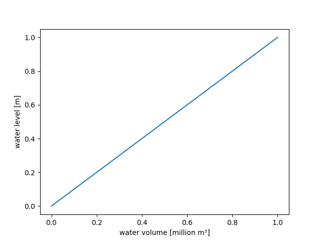
dam_v006 assumes the relationship between WaterLevel and WaterVolume to be
constant over time. For simplicity, we define a linear relationship by using PPoly:
>>> watervolume2waterlevel(PPoly.from_data(xs=[0.0, 1.0], ys=[0.0, 1.0]))
>>> figure = watervolume2waterlevel.plot(0.0, 1.0)
>>> from hydpy.core.testtools import save_autofig
>>> save_autofig("dam_v006_watervolume2waterlevel.png", figure=figure)
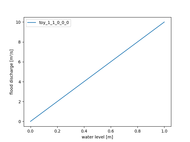
dam_v006 uses parameter WaterLevel2FloodDischarge (which extends parameter
SeasonalInterpolator) to allow for annual changes in the relationship between
FloodDischarge and WaterLevel. Please read the documentation on class
SeasonalInterpolator on how to model seasonal patterns. Here, we keep things as
simple as possible and define a single linear relationship that applies for the whole
year:
>>> waterlevel2flooddischarge(PPoly.from_data(xs=[0.0, 1.0], ys=[0.0, 10.0]))
>>> figure = waterlevel2flooddischarge.plot(0.0, 1.0)
>>> figure = save_autofig("dam_v006_waterlevel2flooddischarge.png", figure=figure)
The following group of parameters deal with lake precipitation and evaporation. Note
that, despite dam_v006’s ability to calculate the water-level dependent surface area
(see aide sequence SurfaceArea), it always assumes a fixed surface area
(defined by control parameter SurfaceArea) for converting precipitation
and evaporation heights into volumes. Here, we set this fixed surface area to 1.44 km²:
>>> surfacearea(1.44)
We set the correction factors for precipitation and evaporation both to 1.2:
>>> correctionprecipitation(1.2)
>>> correctionevaporation(1.2)
Given the daily simulation time step, we configure moderate damping and delay of the external evaporation values (0.8 is relatively close to 1.0, which would avoid any delay and damping, while 0.0 would result in a complete loss of variability):
>>> weightevaporation(0.8)
dam_v006 uses the parameter ThresholdEvaporation for defining the water level
around which actual evaporation switches from zero to potential evaporation. As usual
but not mandatory, we set this threshold to 0 m:
>>> thresholdevaporation(0.0)
Additionally, we set the values of the related smoothing parameters DischargeTolerance
and ToleranceEvaporation to 0.1 m³/s and 1 mm (these are values we can recommend
for many cases – see the documentation on application model dam_v001 on how to
fine-tune such smoothing parameters to your needs):
>>> dischargetolerance(0.1)
>>> toleranceevaporation(0.001)
Finally, we define a precipitation series including only a heavy one-day rainfall event and a corresponding inflowing flood wave, starting and ending with zero discharge:
>>> inputs.precipitation.series = [
...     0.0, 50.0, 0.0, 0.0, 0.0, 0.0, 0.0, 0.0, 0.0, 0.0,
...     0.0, 0.0, 0.0, 0.0, 0.0, 0.0, 0.0, 0.0, 0.0, 0.0]
>>> lake.inlets.inflow.sequences.sim.series = [
...     0.0, 0.0, 6.0, 12.0, 10.0, 6.0, 3.0, 2.0, 1.0, 0.0,
...     0.0, 0.0, 0.0, 0.0, 0.0, 0.0, 0.0, 0.0, 0.0, 0.0]
base scenario
For our first example, we set the allowed water level drop to inf and the
external potential evaporation as well as the exchange values to zero to ensure they do
not affect the calculated lake outflow:
>>> allowedwaterleveldrop(inf)
>>> inputs.evaporation.series = 0.0
>>> exchange.sequences.sim.series = 0.0
The only purpose of parameter CatchmentArea is to determine reasonable default values
for the parameter AbsErrorMax automatically, controlling the accuracy of the numerical
integration process:
>>> catchmentarea(86.4)
>>> from hydpy import round_
>>> round_(solver.abserrormax.INIT)
0.01
>>> parameters.update()
>>> solver.abserrormax
abserrormax(0.01)
The following test results show the expected storage retention pattern. The sums of inflow and outflow are nearly identical, and the maximum of the outflow graph intersects with the falling limb of the inflow graph:
>>> test("dam_v006_base_scenario")
Click to see the table
Click to see the graphdam_v006 achieves this sufficiently high accuracy with 174 calls to
its underlying system of differential equations, which averages to less
than nine calls per day:
>>> model.numvars.nmb_calls
174
There is no indication of an error in the water balance:
>>> from hydpy import round_
>>> round_(model.check_waterbalance(conditions))
0.0
low accuracy
By increasing the numerical tolerance, e.g. setting AbsErrorMax to 0.1 m³/s, we gain
some additional speedups without relevant deteriorations of the results (dam_v006
usually achieves higher accuracies than indicated by the actual tolerance value):
>>> model.numvars.nmb_calls = 0
>>> solver.abserrormax(0.1)
>>> test("dam_v006_low_accuracy")
Click to see the table
Click to see the graph>>> model.numvars.nmb_calls
104
There is no indication of an error in the water balance:
>>> round_(model.check_waterbalance(conditions))
0.0
water level drop
When setting AllowedWaterLevelDrop to 0.1 m/d, the resulting outflow hydrograph shows
a plateau in its falling limb. This plateau is in the period where little inflow
occurs, but the potential outflow (FloodDischarge) is still high due to large amounts
of stored water. In agreement with the linear relationship between the water volume
and the water level, there is a constant decrease in the water volume when the allowed
water level drop limits the outflow:
>>> allowedwaterleveldrop(0.1)
>>> solver.abserrormax(0.01)
>>> test("dam_v006_water_level_drop")
Click to see the table
Click to see the graphThere is no indication of an error in the water balance:
>>> round_(model.check_waterbalance(conditions))
0.0
evaporation
In this example, we set the (unadjusted) potential evaporation to 1 mm/d for the first ten days and 5 mm/d for the last ten days. The adjusted evaporation follows the given potential evaporation with a short delay. When the water volume reaches zero, actual evaporation is nearly but, due to the defined smoothing, not completely zero. Hence, slightly negative water volumes result (which do not cause negative outflow):
>>> inputs.evaporation.series = 10 * [1.0] + 10 * [5.0]
>>> test("dam_v006_evaporation")
Click to see the table
Click to see the graphThere is no indication of an error in the water balance:
>>> round_(model.check_waterbalance(conditions))
0.0
exchange
The water exchange functionality of dam_v006 is optional insofar that one does not
need to connect the inlet sequence E to any nodes. If there is a connection to one
or multiple nodes, they can add and subtract water, indicated by positive or negative
values. This mechanism allows establishing bidirectional water exchange between
different dam_v006 (see the documentation exch_v001 for further information).
dam_v006 handles the water exchange strictly as input, meaning it always includes it
into its water balance without any modification. Hence, other models calculating the
water exchange must ensure that it does not bring dam_v006 into an unrealistic state.
For demonstration, we set the water exchange to 0.5 m³/s in the first half of the
simulation period and -0.5 m³/s in the second half, which causes highly negative water
volumes at the end of the simulation period:
>>> exchange.sequences.sim.series = 10 * [0.5] + 10 * [-0.5]
>>> test("dam_v006_exchange")
Click to see the table
Click to see the graph>>> round_(model.check_waterbalance(conditions))
0.0
- class hydpy.models.dam_v006.Model[source]
Bases:
ELSModelVersion 6 of HydPy-Dam.
- The following “inlet update methods” are called in the given sequence at the beginning of each simulation step:
Calc_AdjustedEvaporation_V1Adjust the given potential evaporation.
- The following methods define the relevant components of a system of ODE equations (e.g. direct runoff):
Calc_AdjustedPrecipitation_V1Adjust the given precipitation.Pic_Inflow_V1Update the inlet sequenceInflow.Pic_Exchange_V1Update the inlet sequenceExchange.Calc_WaterLevel_V1Determine the water level based on an interpolation approach approximating the relationship between water volume and water level.Calc_ActualEvaporation_V1Calculate the actual evaporation.Calc_SurfaceArea_V1Determine the surface area based on an interpolation approach approximating the relationship between water level and the surface area.Calc_FloodDischarge_V1Calculate the discharge during and after a flood event based on seasonally varying interpolation approaches approximating the relationship(s) between discharge and water stage.Calc_AllowedDischarge_V1Calculate the maximum discharge not leading to exceedance of the allowed water level drop.Calc_Outflow_V2Calculate the total outflow of the dam, taking the allowed water discharge into account.
- The following methods define the complete equations of an ODE system (e.g. change in storage of fast water due to effective precipitation and direct runoff):
Update_WaterVolume_V4Update the actual water volume.
- The following “outlet update methods” are called in the given sequence at the end of each simulation step:
Calc_WaterLevel_V1Determine the water level based on an interpolation approach approximating the relationship between water volume and water level.Pass_Outflow_V1Update the outlet link sequenceQ.
- The following “additional methods” might be called by one or more of the other methods or are meant to be directly called by the user:
Fix_Min1_V1Apply functionsmooth_min1()without risking negative results.
- check_waterbalance(initial_conditions: Dict[str, Dict[str, ArrayFloat]]) float[source]
Determine the water balance error of the previous simulation run in million m³.
Method
check_waterbalance()calculates the balance error as follows:\(Seconds \cdot 10^{-6} \cdot \sum_{t=t0}^{t1} \big( AdjustedPrecipitation_t - ActualEvaporation_t + Inflow_t - Outflow_t + Exchange_t \big) + \big( WaterVolume_{t0}^k - WaterVolume_{t1}^k \big)\)
The returned error should always be in scale with numerical precision so that it does not affect the simulation results in any relevant manner.
Pick the required initial conditions before starting the simulation run via property
conditions. See the integration tests of the application modeldam_v006for some examples.
- class hydpy.models.dam_v006.AideSequences(master: Sequences, cls_fastaccess: Type[TypeFastAccess_co] | None = None, cymodel: CyModelProtocol | None = None)
Bases:
AideSequencesAide sequences of model dam_v006.
- The following classes are selected:
SurfaceArea()Surface area [km²].AllowedDischarge()Discharge threshold not to be overcut by the actual discharge [m³/s].
- class hydpy.models.dam_v006.ControlParameters(master: Parameters, cls_fastaccess: Type[FastAccessParameter] | None = None, cymodel: CyModelProtocol | None = None)
Bases:
SubParametersControl parameters of model dam_v006.
- The following classes are selected:
SurfaceArea()Average size of the water surface [km²].CatchmentArea()Size of the catchment draining into the dam [km²].CorrectionPrecipitation()Precipitation correction factor [-].CorrectionEvaporation()Evaporation correction factor [-].WeightEvaporation()Time weighting factor for evaporation [-].ThresholdEvaporation()The water level at which actual evaporation is 50 % of potential evaporation [m].ToleranceEvaporation()A tolerance value defining the steepness of the transition of actual evaporation between zero and potential evaporation [m].WaterVolume2WaterLevel()Artificial neural network describing the relationship between water level and water volume [-].WaterLevel2FloodDischarge()Artificial neural network describing the relationship between flood discharge and water volume [-].AllowedWaterLevelDrop()The highest allowed water level decrease [m/T].DischargeTolerance()Smoothing parameter for discharge related smoothing operations [m³/s].
- class hydpy.models.dam_v006.DerivedParameters(master: Parameters, cls_fastaccess: Type[FastAccessParameter] | None = None, cymodel: CyModelProtocol | None = None)
Bases:
SubParametersDerived parameters of model dam_v006.
- The following classes are selected:
TOY()References thetimeofyearindex array provided by the instance of classIndexeravailable in modulepub[-].Seconds()Length of the actual simulation step size [s].InputFactor()Factor for converting meteorological input from mm/T to million m³/s.SmoothParEvaporation()Smoothing parameter to be derived fromToleranceEvaporationfor smoothing kernelsmooth_logistic1()[m].DischargeSmoothPar()Smoothing parameter to be derived fromDischargeTolerancefor smoothing kernelssmooth_min1()andsmooth_max1()[m³/s].
- class hydpy.models.dam_v006.FactorSequences(master: Sequences, cls_fastaccess: Type[TypeFastAccess_co] | None = None, cymodel: CyModelProtocol | None = None)
Bases:
FactorSequencesFactor sequences of model dam_v006.
- The following classes are selected:
WaterLevel()Water level [m].
- class hydpy.models.dam_v006.FluxSequences(master: Sequences, cls_fastaccess: Type[TypeFastAccess_co] | None = None, cymodel: CyModelProtocol | None = None)
Bases:
FluxSequencesFlux sequences of model dam_v006.
- The following classes are selected:
AdjustedPrecipitation()Adjusted precipitation [m³/s].AdjustedEvaporation()Adjusted evaporation [m³/s].ActualEvaporation()Actual evaporation [m³/s].Inflow()Total inflow [m³/s].Exchange()Water exchange with another location [m³/s].FloodDischarge()Water release associated with flood events [m³/s].Outflow()Total outflow [m³/s].
- class hydpy.models.dam_v006.InletSequences(master: Sequences, cls_fastaccess: Type[TypeFastAccess_co] | None = None, cymodel: CyModelProtocol | None = None)
Bases:
InletSequencesInlet sequences of model dam_v006.
- class hydpy.models.dam_v006.InputSequences(master: Sequences, cls_fastaccess: Type[TypeFastAccess_co] | None = None, cymodel: CyModelProtocol | None = None)
Bases:
InputSequencesInput sequences of model dam_v006.
- The following classes are selected:
Precipitation()Precipitation [mm].Evaporation()Potential evaporation [mm].
- class hydpy.models.dam_v006.LogSequences(master: Sequences, cls_fastaccess: Type[TypeFastAccess_co] | None = None, cymodel: CyModelProtocol | None = None)
Bases:
LogSequencesLog sequences of model dam_v006.
- The following classes are selected:
LoggedAdjustedEvaporation()Logged adjusted evaporation [m3/s].
- class hydpy.models.dam_v006.OutletSequences(master: Sequences, cls_fastaccess: Type[TypeFastAccess_co] | None = None, cymodel: CyModelProtocol | None = None)
Bases:
OutletSequencesOutlet sequences of model dam_v006.
- The following classes are selected:
Q()Outflow [m³/s].
- class hydpy.models.dam_v006.SolverParameters(master: Parameters, cls_fastaccess: Type[FastAccessParameter] | None = None, cymodel: CyModelProtocol | None = None)
Bases:
SubParametersSolver parameters of model dam_v006.
- The following classes are selected:
AbsErrorMax()Absolute numerical error tolerance [m³/s].RelErrorMax()Relative numerical error tolerance [1/T].RelDTMin()Smallest relative integration time step size allowed [-].RelDTMax()Largest relative integration time step size allowed [-].
- class hydpy.models.dam_v006.StateSequences(master: Sequences, cls_fastaccess: Type[TypeFastAccess_co] | None = None, cymodel: CyModelProtocol | None = None)
Bases:
StateSequencesState sequences of model dam_v006.
- The following classes are selected:
WaterVolume()Water volume [million m³].