dam_v004
Version 4 of HydPy-Dam.
Application model dam_v004 extends dam_v003. Both models discharge water into the
channel downstream and to “remote locations”. The difference is that dam_v003
releases water only to a single remote location (for example, to a drinking water
treatment plant) while dam_v004 also discharges to a second remote location (for
example, to relieve water during high flow conditions).
The following explanations focus on this difference. For further information on using
dam_v004, please read the documentation on dam_v001 and dam_v003. Besides that,
consider reading the documentation on dam_v005, which is a possible counterpart to
dam_v004, being able to send information on required supply and allowed relief and to
consume the related discharges.
Integration tests
Note
When new to HydPy, consider reading section How to understand integration tests? first.
The following examples stem from the documentation of application model dam_v003.
Some are recalculations to confirm the proper implementation of the features common
to both models. Others are modifications that illustrate the additional features
of dam_v003.
The time-related setup is identical to the one of dam_v003:
>>> from hydpy import pub, Node, Element
>>> pub.timegrids = "01.01.2000", "21.01.2000", "1d"
In addition to the general configuration of application model dam_v003, we require
connections to two additional Node objects. Node allowed_relief provides
information on the maximum allowed relief discharge, and node actual_relief passes
the actual relief discharge to a remote location. Both nodes use the string literal “R”
to connect to the receiver sequence R and the outlet sequence
R, respectively:
>>> inflow = Node("inflow", variable="Q")
>>> outflow = Node("outflow", variable="Q")
>>> required_supply = Node("required_supply", variable="S")
>>> actual_supply = Node("actual_supply", variable="S")
>>> allowed_relief = Node("allowed_relief", variable="R")
>>> actual_relief = Node("actual_relief", variable="R")
>>> dam = Element("dam",
...               inlets=inflow,
...               outlets=(outflow, actual_supply, actual_relief),
...               receivers=(required_supply, allowed_relief))
>>> from hydpy.models.dam_v004 import *
>>> parameterstep("1d")
>>> dam.model = model
We prepare the IntegrationTest object as for dam_v003:
>>> from hydpy import IntegrationTest
>>> test = IntegrationTest(dam)
>>> test.dateformat = "%d.%m."
>>> test.plotting_options.axis1 = fluxes.inflow, fluxes.outflow
>>> test.plotting_options.axis2 = states.watervolume
dam_v004 requires additional initial conditions for the sequence
LoggedAllowedRemoteRelief:
>>> test.inits=((states.watervolume, 0.0),
...             (logs.loggedadjustedevaporation, 0.0),
...             (logs.loggedrequiredremoterelease, 0.005),
...             (logs.loggedallowedremoterelief, 0.0))
We define the same inflow, Precipitation, and Evaporation
time series as for dam_v003:
>>> inflow.sequences.sim.series = 1.0
>>> inputs.precipitation.series = 0.0
>>> inputs.evaporation.series = 0.0
dam_v003 and dam_v004 share the following parameters and we apply the same values
as for dam_v003:
>>> watervolume2waterlevel(PPoly.from_data(xs=[0.0, 1.0], ys=[0.0, 0.25]))
>>> waterlevel2flooddischarge(PPoly.from_data(xs=[0.0], ys=[0.0]))
>>> catchmentarea(86.4)
>>> neardischargeminimumthreshold(0.2)
>>> neardischargeminimumtolerance(0.2)
>>> waterlevelminimumthreshold(0.0)
>>> waterlevelminimumtolerance(0.0)
>>> waterlevelminimumremotethreshold(0.0)
>>> waterlevelminimumremotetolerance(0.0)
>>> restricttargetedrelease(True)
>>> surfacearea(1.44)
>>> correctionprecipitation(1.2)
>>> correctionevaporation(1.2)
>>> weightevaporation(0.8)
>>> thresholdevaporation(0.0)
>>> toleranceevaporation(0.001)
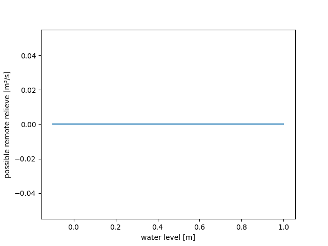
The following parameters are unique to dam_v004. We first set “neutral” values
which disable any relief discharges:
>>> remoterelieftolerance(0.0)
>>> highestremotedischarge(inf)
>>> highestremotetolerance(0.1)
>>> waterlevel2possibleremoterelief(PPoly.from_data(xs=[0.0], ys=[0.0]))
>>> figure = waterlevel2possibleremoterelief.plot(-0.1, 1.0)
>>> from hydpy.core.testtools import save_autofig
>>> save_autofig("dam_v004_waterlevel2possibleremoterelief_1.png", figure=figure)
smooth near minimum
The following examples correspond to the smooth near minimum example of
application model dam_v001 as well as the smooth near minimum example
of application model dam_v003. We again use the same remote demand:
>>> required_supply.sequences.sim.series = [
...     0.008588, 0.010053, 0.013858, 0.027322, 0.064075, 0.235523, 0.470414,
...     0.735001, 0.891263, 0.696325, 0.349797, 0.105231, 0.111928, 0.240436,
...     0.229369, 0.058622, 0.016958, 0.008447, 0.004155, 0.0]
recalculation
To first perform a strict recalculation, we set the allowed discharge relief to zero:
>>> allowed_relief.sequences.sim.series = 0.0
This recalculation confirms that model dam_v004 functions exactly like model dam_v003
to meet the water demands at a cross-section downstream and a single remote location
(for example, see column “waterlevel”):
>>> test("dam_v004_smooth_near_minimum_recalculation",
... axis1=(fluxes.inflow, fluxes.outflow, fluxes.actualremoterelease),
... axis2=states.watervolume)
Click to see the table
Click to see the graphmodification 1
In this first modification of the smooth near minimum example, we take the old required supply as the new allowed relief discharge and set the new required supply to zero:
>>> allowed_relief.sequences.sim.series = required_supply.sequences.sim.series
>>> test.inits.loggedallowedremoterelief = 0.005
>>> required_supply.sequences.sim.series = 0.0
>>> test.inits.loggedrequiredremoterelease = 0.0
Also, we set the possible relief discharge to a huge constant value of 100 m³/s:
>>> waterlevel2possibleremoterelief(PPoly.from_data(xs=[0.0], ys=[100.0]))
>>> figure = waterlevel2possibleremoterelief.plot(-0.1, 1.0)
>>> from hydpy.core.testtools import save_autofig
>>> save_autofig("dam_v004_waterlevel2possibleremoterelief_2.png", figure=figure)
Due to this setting, the new actual relief discharge is nearly identical to the old
actual supply discharge. There is only a minor deviation in the first simulation step
due to the numerical inaccuracy explained in the documentation on dam_v001:
>>> test("dam_v004_smooth_near_minimum_modification_1",
... axis1=(fluxes.inflow, fluxes.outflow, fluxes.actualremoterelief),
... axis2=states.watervolume)
Click to see the table
Click to see the graphmodification 2
Now, we modify WaterLevel2PossibleRemoteRelief to prevent any relief discharge when
the dam is empty and to set its maximum to 0.5 m³/s:
>>> waterlevel2possibleremoterelief(ANN(weights_input=1e30, weights_output=0.5,
...                                     intercepts_hidden=-1e27, intercepts_output=0.0))
>>> waterlevel2possibleremoterelief(PPoly(Poly(x0=-1.0, cs=(0.0,)), Poly(x0=0.0, cs=(0.5,))))
>>> figure = waterlevel2possibleremoterelief.plot(-0.1, 1.0)
>>> from hydpy.core.testtools import save_autofig
>>> save_autofig("dam_v004_waterlevel2possibleremoterelief_3.png", figure=figure)
For low water levels, the current customisation of the possible relief discharge
resembles the customisation of the actual supply defined in the
recalculation example. Hence, the results for
ActualRemoteRelease and ActualRemoteRelief of the respective experiments agree
well (again, except for the minor deviation for the first simulation step due to
limited numerical accuracy). For the high water levels (between January 9 and January
11), the imposed restriction of 0.5 m³/s results in a reduced relief discharge:
>>> test("dam_v004_smooth_near_minimum_modification_2",
... axis1=(fluxes.inflow, fluxes.outflow, fluxes.actualremoterelief),
... axis2=states.watervolume)
Click to see the table
Click to see the graphmodification 3
The restricted possible relief discharge in the example above results in a discontinuous
evolution of the actual relief discharge. To achieve smoother transitions, one can set
RemoteReliefTolerance to a value larger than zero:
>>> remoterelieftolerance(0.2)
>>> test("dam_v004_smooth_near_minimum_modification_3",
... axis1=(fluxes.inflow, fluxes.outflow, fluxes.actualremoterelief),
... axis2=states.watervolume)
Click to see the table
Click to see the graphrestriction enabled
The following exact recalculations demonstrate the identical functioning of those
components of dam_v004 and dam_v003 not utilised in the examples above. Therefore,
we disable the remote relief discharge again:
>>> test.inits.loggedrequiredremoterelease = 0.005
>>> test.inits.loggedallowedremoterelief = 0.0
>>> waterlevelminimumremotetolerance(0.0)
>>> waterlevel2possibleremoterelief(PPoly.from_data(xs=[0.0], ys=[0.0]))
>>> remoterelieftolerance(0.0)
>>> allowed_relief.sequences.sim.series = 0.0
Here, we confirm equality when releasing water to the channel downstream during low flow conditions. We need to update the time series of the inflow and the required remote release:
>>> inflow.sequences.sim.series[10:] = 0.1
>>> required_supply.sequences.sim.series = [
...     0.008746, 0.010632, 0.015099, 0.03006, 0.068641, 0.242578, 0.474285, 0.784512,
...     0.95036, 0.35, 0.034564, 0.299482, 0.585979, 0.557422, 0.229369, 0.142578,
...     0.068641, 0.029844, 0.012348, 0.0]
>>> neardischargeminimumtolerance(0.0)
The following results agree with the test results of the
restriction enabled example of application model dam_v003:
>>> test("dam_v004_restriction_enabled")
Click to see the table
Click to see the graphsmooth stage minimum
This example repeats the smooth stage minimum example of application
model dam_v003. We update all parameter and time series accordingly:
>>> waterlevelminimumtolerance(0.01)
>>> waterlevelminimumthreshold(0.005)
>>> waterlevelminimumremotetolerance(0.01)
>>> waterlevelminimumremotethreshold(0.01)
>>> inflow.sequences.sim.series = numpy.linspace(0.2, 0.0, 20)
>>> required_supply.sequences.sim.series = [
...     0.01232, 0.029323, 0.064084, 0.120198, 0.247367, 0.45567, 0.608464,
...     0.537314, 0.629775, 0.744091, 0.82219, 0.841916, 0.701812, 0.533258,
...     0.351863, 0.185207, 0.107697, 0.055458, 0.025948, 0.0]
dam_v004 responds equally to limited storage contents as dam_v003:
>>> test("dam_v004_smooth_stage_minimum")
Click to see the table
Click to see the graphevaporation
This example repeats the evaporation example of application model
dam_v003. We update the time series of potential evaporation and the required remote
release accordingly:
>>> inputs.evaporation.series = 10 * [1.0] + 10 * [5.0]
>>> required_supply.sequences.sim.series = [
...     0.012321, 0.029352, 0.064305, 0.120897, 0.248435, 0.453671, 0.585089,
...     0.550583, 0.694398, 0.784979, 0.81852, 0.840207, 0.72592, 0.575373,
...     0.386003, 0.198088, 0.113577, 0.05798, 0.026921, 0.0]
>>> test("dam_v004_evaporation")
Click to see the table
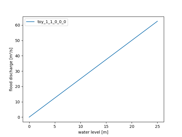
Click to see the graphflood retention
The following examples correspond to the flood retention example of
application model dam_v001 as well as the flood retention example
of application model dam_v003. We use the same parameter and input time series
configuration:
>>> neardischargeminimumthreshold(0.0)
>>> neardischargeminimumtolerance(0.0)
>>> waterlevelminimumthreshold(0.0)
>>> waterlevelminimumtolerance(0.0)
>>> waterlevelminimumremotethreshold(0.0)
>>> waterlevelminimumremotetolerance(0.0)
>>> waterlevel2flooddischarge(PPoly.from_data(xs=[0.0, 1.0], ys=[0.0, 2.5]))
>>> neardischargeminimumthreshold(0.0)
>>> inputs.precipitation.series = [0.0, 50.0, 0.0, 0.0, 0.0, 0.0, 0.0, 0.0, 0.0, 0.0,
...                                0.0, 0.0, 0.0, 0.0, 0.0, 0.0, 0.0, 0.0, 0.0, 0.0]
>>> inflow.sequences.sim.series = [0.0, 0.0, 5.0, 9.0, 8.0, 5.0, 3.0, 2.0, 1.0, 0.0,
...                                0.0, 0.0, 0.0, 0.0, 0.0, 0.0, 0.0, 0.0, 0.0, 0.0]
>>> inputs.evaporation.series = 0.0
recalculation
To first perform a strict recalculation, we set the remote demand to zero (the allowed relief is already zero):
>>> required_supply.sequences.sim.series = 0.0
>>> test.inits.loggedrequiredremoterelease = 0.0
>>> allowed_relief.sequences.sim.series
InfoArray([0., ..., 0.])
The following results demonstrate that dam_v003 calculates the same outflow values as
dam_v001 and dam_v003 in situations where the remote locations are inactive:
>>> test("dam_v004_flood_retention_recalculation")
Click to see the table
Click to see the graphmodification
Building on the example above, we demonstrate the possibility to constrain the total
discharge to remote locations by setting HighestRemoteDischarge to 1.0 m³/s, which
defines the allowed sum of AllowedRemoteRelief and ActualRemoteRelease:
>>> highestremotedischarge(1.0)
>>> highestremotetolerance(0.1)
This final example demonstrates the identical behaviour of models
dam_v003 and dam_v004 (and also of models dam_v001 and
dam_v002 regarding high flow conditions:
We assume a constant remote demand of 0.5 m³/s and let the allowed relief rise linearly from 0.0 to 1.5 m³/s:
>>> required_supply.sequences.sim.series = 0.5
>>> test.inits.loggedrequiredremoterelease = 0.5
>>> allowed_relief.sequences.sim.series = numpy.linspace(0.0, 1.5, 20)
>>> test.inits.loggedallowedremoterelief = 0.0
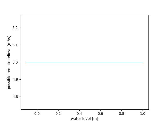
Also, we set the possible relief discharge to a constant value of 5.0 m³/s:
>>> waterlevel2possibleremoterelief(PPoly.from_data(xs=[0.0], ys=[5.0]))
>>> figure = waterlevel2possibleremoterelief.plot(-0.1, 1.0)
>>> save_autofig("dam_v004_waterlevel2possibleremoterelief_4.png", figure=figure)
The following results demonstrate that AllowedRemoteRelief has priority over
ActualRemoteRelease. Due to parameter HighestRemoteDischarge set to 1.0 m³/s,
ActualRemoteRelease starts to drop when AllowedRemoteRelief exceeds 0.5 m³/s.
Furthermore, AllowedRemoteRelief itself never exceeds 1.0 m³/s:
>>> test("dam_v004_flood_retention_modification")
Click to see the table
Click to see the graph- class hydpy.models.dam_v004.Model[source]
Bases:
ELSModelVersion 4 of HydPy-Dam.
- The following “receiver update methods” are called in the given sequence before performing a simulation step:
Pic_LoggedRequiredRemoteRelease_V2Update the receiver sequenceLoggedRequiredRemoteRelease.Pic_LoggedAllowedRemoteRelief_V1Update the receiver sequenceLoggedAllowedRemoteRelief.
- The following “inlet update methods” are called in the given sequence at the beginning of each simulation step:
Calc_AdjustedEvaporation_V1Adjust the given potential evaporation.Pic_Inflow_V1Update the inlet sequenceInflow.Calc_RequiredRemoteRelease_V2Get the required remote release of the last simulation step.Calc_AllowedRemoteRelief_V1Get the allowed remote relief of the last simulation step.Calc_RequiredRelease_V2Calculate the water release (immediately downstream) required for reducing drought events.Calc_TargetedRelease_V1Calculate the targeted water release for reducing drought events, taking into account both the required water release and the actual inflow into the dam.
- The following methods define the relevant components of a system of ODE equations (e.g. direct runoff):
Calc_AdjustedPrecipitation_V1Adjust the given precipitation.Pic_Inflow_V1Update the inlet sequenceInflow.Calc_WaterLevel_V1Determine the water level based on an interpolation approach approximating the relationship between water volume and water level.Calc_ActualEvaporation_V1Calculate the actual evaporation.Calc_ActualRelease_V1Calculate the actual water release that can be supplied by the dam considering the targeted release and the given water level.Calc_PossibleRemoteRelief_V1Calculate the highest possible water release that can be routed to a remote location based on an interpolation approach approximating the relationship between possible release and water stage.Calc_ActualRemoteRelief_V1Calculate the actual amount of water released to a remote location to relieve the dam during high flow conditions.Calc_ActualRemoteRelease_V1Calculate the actual remote water release that can be supplied by the dam considering the required remote release and the given water level.Update_ActualRemoteRelease_V1Constrain the actual release (supply discharge) to a remote location.Update_ActualRemoteRelief_V1Constrain the actual relief discharge to a remote location.Calc_FloodDischarge_V1Calculate the discharge during and after a flood event based on seasonally varying interpolation approaches approximating the relationship(s) between discharge and water stage.Calc_Outflow_V1Calculate the total outflow of the dam.
- The following methods define the complete equations of an ODE system (e.g. change in storage of fast water due to effective precipitation and direct runoff):
Update_WaterVolume_V3Update the actual water volume.
- The following “outlet update methods” are called in the given sequence at the end of each simulation step:
Calc_WaterLevel_V1Determine the water level based on an interpolation approach approximating the relationship between water volume and water level.Pass_Outflow_V1Update the outlet link sequenceQ.Pass_ActualRemoteRelease_V1Update the outlet link sequenceS.Pass_ActualRemoteRelief_V1Update the outlet link sequenceR.
- The following “additional methods” might be called by one or more of the other methods or are meant to be directly called by the user:
Fix_Min1_V1Apply functionsmooth_min1()without risking negative results.
- class hydpy.models.dam_v004.ControlParameters(master: Parameters, cls_fastaccess: Type[FastAccessParameter] | None = None, cymodel: CyModelProtocol | None = None)
Bases:
SubParametersControl parameters of model dam_v004.
- The following classes are selected:
SurfaceArea()Average size of the water surface [km²].CatchmentArea()Size of the catchment draining into the dam [km²].CorrectionPrecipitation()Precipitation correction factor [-].CorrectionEvaporation()Evaporation correction factor [-].WeightEvaporation()Time weighting factor for evaporation [-].WaterLevel2PossibleRemoteRelief()Artificial neural network describing the relationship between water level and the highest possible water release used to relieve the dam during high flow conditions [-].RemoteReliefTolerance()A tolerance value forPossibleRemoteRelief[m³/s].NearDischargeMinimumThreshold()Discharge threshold of a cross-section near the dam not to be undercut by the actual discharge [m³/s].NearDischargeMinimumTolerance()A tolerance value for the “near discharge minimum” [m³/s].RestrictTargetedRelease()A flag indicating whether low flow variability has to be preserved or not [-].WaterLevelMinimumThreshold()The minimum operating water level of the dam [m].WaterLevelMinimumTolerance()A tolerance value for the minimum operating water level [m].ThresholdEvaporation()The water level at which actual evaporation is 50 % of potential evaporation [m].ToleranceEvaporation()A tolerance value defining the steepness of the transition of actual evaporation between zero and potential evaporation [m].WaterLevelMinimumRemoteThreshold()The minimum operating water level of the dam regarding remote water supply [m].WaterLevelMinimumRemoteTolerance()A tolerance value for the minimum operating water level regarding remote water supply [m].HighestRemoteDischarge()The highest possible discharge between two remote locations [m³/s].HighestRemoteTolerance()Smoothing parameter associated withHighestRemoteDischarge[m³/s].WaterVolume2WaterLevel()Artificial neural network describing the relationship between water level and water volume [-].WaterLevel2FloodDischarge()Artificial neural network describing the relationship between flood discharge and water volume [-].
- class hydpy.models.dam_v004.DerivedParameters(master: Parameters, cls_fastaccess: Type[FastAccessParameter] | None = None, cymodel: CyModelProtocol | None = None)
Bases:
SubParametersDerived parameters of model dam_v004.
- The following classes are selected:
TOY()References thetimeofyearindex array provided by the instance of classIndexeravailable in modulepub[-].Seconds()Length of the actual simulation step size [s].InputFactor()Factor for converting meteorological input from mm/T to million m³/s.NearDischargeMinimumSmoothPar1()Smoothing parameter to be derived fromNearDischargeMinimumThresholdfor smoothing kernelsmooth_logistic1()[m³/s].WaterLevelMinimumSmoothPar()Smoothing parameter to be derived fromWaterLevelMinimumTolerancefor smoothing kernelsmooth_logistic1()[m].SmoothParEvaporation()Smoothing parameter to be derived fromToleranceEvaporationfor smoothing kernelsmooth_logistic1()[m].WaterLevelMinimumRemoteSmoothPar()Smoothing parameter to be derived fromWaterLevelMinimumRemoteTolerance[m].HighestRemoteSmoothPar()Smoothing parameter to be derived fromHighestRemoteTolerancefor smoothing kernelsmooth_min1()[m³/s].
- class hydpy.models.dam_v004.FactorSequences(master: Sequences, cls_fastaccess: Type[TypeFastAccess_co] | None = None, cymodel: CyModelProtocol | None = None)
Bases:
FactorSequencesFactor sequences of model dam_v004.
- The following classes are selected:
WaterLevel()Water level [m].
- class hydpy.models.dam_v004.FluxSequences(master: Sequences, cls_fastaccess: Type[TypeFastAccess_co] | None = None, cymodel: CyModelProtocol | None = None)
Bases:
FluxSequencesFlux sequences of model dam_v004.
- The following classes are selected:
AdjustedPrecipitation()Adjusted precipitation [m³/s].AdjustedEvaporation()Adjusted evaporation [m³/s].ActualEvaporation()Actual evaporation [m³/s].Inflow()Total inflow [m³/s].RequiredRemoteRelease()Water release considered appropriate to reduce drought events at cross-sections far downstream [m³/s].AllowedRemoteRelief()Allowed discharge to relieve a dam during high flow conditions [m³/s].PossibleRemoteRelief()Maximum possible water release to a remote location to relieve the dam during high flow conditions [m³/s].ActualRemoteRelief()Actual water release to a remote location to relieve the dam during high flow conditions [m³/s].RequiredRelease()Required water release for reducing drought events downstream [m³/s].TargetedRelease()The targeted water release for reducing drought events downstream after taking both the required release and additional low flow regulations into account [m³/s].ActualRelease()Actual water release thought for reducing drought events downstream [m³/s].ActualRemoteRelease()Actual water release thought for arbitrary “remote” purposes [m³/s].FloodDischarge()Water release associated with flood events [m³/s].Outflow()Total outflow [m³/s].
- class hydpy.models.dam_v004.InletSequences(master: Sequences, cls_fastaccess: Type[TypeFastAccess_co] | None = None, cymodel: CyModelProtocol | None = None)
Bases:
InletSequencesInlet sequences of model dam_v004.
- The following classes are selected:
Q()Inflow [m³/s].
- class hydpy.models.dam_v004.InputSequences(master: Sequences, cls_fastaccess: Type[TypeFastAccess_co] | None = None, cymodel: CyModelProtocol | None = None)
Bases:
InputSequencesInput sequences of model dam_v004.
- The following classes are selected:
Precipitation()Precipitation [mm].Evaporation()Potential evaporation [mm].
- class hydpy.models.dam_v004.LogSequences(master: Sequences, cls_fastaccess: Type[TypeFastAccess_co] | None = None, cymodel: CyModelProtocol | None = None)
Bases:
LogSequencesLog sequences of model dam_v004.
- The following classes are selected:
LoggedAdjustedEvaporation()Logged adjusted evaporation [m3/s].LoggedRequiredRemoteRelease()Logged required discharge values computed by another model [m3/s].LoggedAllowedRemoteRelief()Logged allowed discharge values computed by another model [m3/s].
- class hydpy.models.dam_v004.OutletSequences(master: Sequences, cls_fastaccess: Type[TypeFastAccess_co] | None = None, cymodel: CyModelProtocol | None = None)
Bases:
OutletSequencesOutlet sequences of model dam_v004.
- class hydpy.models.dam_v004.ReceiverSequences(master: Sequences, cls_fastaccess: Type[TypeFastAccess_co] | None = None, cymodel: CyModelProtocol | None = None)
Bases:
ReceiverSequencesReceiver sequences of model dam_v004.
- class hydpy.models.dam_v004.SolverParameters(master: Parameters, cls_fastaccess: Type[FastAccessParameter] | None = None, cymodel: CyModelProtocol | None = None)
Bases:
SubParametersSolver parameters of model dam_v004.
- The following classes are selected:
AbsErrorMax()Absolute numerical error tolerance [m³/s].RelErrorMax()Relative numerical error tolerance [1/T].RelDTMin()Smallest relative integration time step size allowed [-].RelDTMax()Largest relative integration time step size allowed [-].
- class hydpy.models.dam_v004.StateSequences(master: Sequences, cls_fastaccess: Type[TypeFastAccess_co] | None = None, cymodel: CyModelProtocol | None = None)
Bases:
StateSequencesState sequences of model dam_v004.
- The following classes are selected:
WaterVolume()Water volume [million m³].