wland_v001
Version 1 of HydPy-W-Land is a slightly modified and extended version of the
WALRUS model, specifically designed to simulate surface water fluxes in lowland
catchments influenced by near-surface groundwater [3]. We
implemented wland_v001 on behalf of the German Federal Institute of Hydrology
(BfG) in the context of optimising the control of the Kiel Canal (Nord-Ostsee-Kanal).
With identical parameter values, WALRUS and wland_v001 yield very similar
results for the tutorial data available within the WALRUS repository. We found all
of the relatively small differences were due to using different numerical
integration algorithms, not to differences in the underlying differential equations
(we discuss the only exception to this in the documentation on method Calc_CDG_V1).
However, to keep our extensions consistent, we found it necessary to adjust a few
variable names and some unit conversions related to the size of some subareas.
Our extensions focus on the hydrological processes that apply before precipitation reaches the vadose zone:
We add some factors to correct or adapt the meteorological input data.
We introduce simple storages for intercepted water and snow, implemented similarly as in
lland_v1andlland_v2.We support the specification of hydrological response units for these processes, making
wland_v001a semi-distributed model (but we model the vadose zone in agreement with WALRUS still in a lumped manner).We define the land-use type
SEALED, which has no vadose zone and routes all water reaching the soil surface directly into the quickflow reservoir.We allow specifying subbasins consisting of surface water areas or combinations of surface water and sealed areas only, not possessing any to “vadose zone area” (however, we do not allow specifying subbasins without any surface water area).
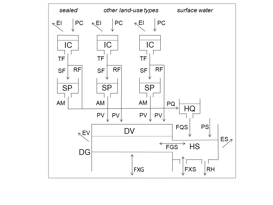
The following figure shows the general structure of wland_v001. Note that, besides
surface water areas and sealed surfaces, all land-use types rely on the same set of
process equations:
The WALRUS model defines some discontinuous differential equations, which
complicate numerical integration [3]. We applied the
regularisation techniques provided by the modules smoothutils and smoothtools
to remove these discontinuities. As shown for each equation (for example, in the
documentation on method Calc_RH_V1), this smoothing is optional. Set the related
parameters SH and ST to zero to disable smoothing, so that the original WALRUS
relationships apply. The larger their values, the faster and more robust the
performance of the numerical integration algorithm, but the larger the discrepancies
to the discontinuous relationships. Our advice is to set small values like 1 mm or
1 °C (as in the following example calculations), respectively, which means that
there is no sharp transition from one behaviour to another at a certain threshold
but a smooth transition that mainly takes place in an interval of about 2 mm or 2 °C
around the threshold. As a consequence, a negative value for the amount of water
stored in the interception storage is acceptable, as the threshold of 0 mm does not
mean that the storage is completely empty but that two domains (the storage is empty
and the storage is not empty) are equally true (similar as in fuzzy logic).
Integration tests
Note
When new to HydPy, consider reading section How to understand integration tests? first.
We perform all simulation runs over the same period of two months with a daily simulation step size:
>>> from hydpy import IntegrationTest, Element, pub, round_
>>> pub.timegrids = "2017-02-10", "2017-04-10", "1d"
wland_v001 usually reads all its input data from disk, making the definition
of the relevant Element object straightforward:
>>> from hydpy.models.wland_v001 import *
>>> parameterstep("1d")
>>> land = Element("land", outlets="outlet")
>>> land.model = model
Our virtual test catchment has 10 km², with a land area of 9.8 km² and a surface water area of 0.2 km²:
>>> al(9.8)
>>> as_(0.2)
We divide the land area into three hydrological of type FIELD, CONIFER, and
SEALED:
>>> nu(3)
>>> lt(FIELD, CONIFER, SEALED)
The relative sizes of the response units relate to the land area-fraction of the test catchment. With the following setting, the total area of the vadose zone is \((0.6 + 0.3) \cdot 9.8 km² = 8.82 km²\):
>>> aur(0.6, 0.3, 0.1)
The following parameter values lead to good results in a small catchment in the
vicinity of the Kiel Canal (northern part of Germany). For those parameters with
land-use specific values (CPETL and LAI), we define only those values relevant
for FIELD, CONIFER, and SEALED. We adopt the default values for the
“physical” soil parameters (B, PsiAE, and ThetaS):
>>> cp(0.8)
>>> cpet(0.9)
>>> cpetl.sealed = 0.7
>>> cpetl.conifer = 1.3
>>> cpetl.field = 0.73, 0.73, 0.77, 0.95, 1.19, 1.18, 1.19, 1.15, 0.97, 0.85, 0.78, 0.73
>>> cpes(jan=1.16, feb=1.22, mar=1.26, apr=1.28, may=1.28, jun=1.30,
...      jul=1.28, aug=1.28, sep=1.27, oct=1.23, nov=1.17, dec=1.14)
>>> lai.sealed = 10.0
>>> lai.conifer = 11.0
>>> lai.field = 0.4, 0.4, 0.3, 0.7, 3.0, 5.2, 4.6, 3.1, 1.3, 0.2, 0.0, 0.0
>>> ih(0.2)
>>> tt(0.0)
>>> ti(4.0)
>>> ddf(5.0)
>>> ddt(0.0)
>>> cw(400.0)
>>> cv(0.2)
>>> cg(200000.0)
>>> cgf(1.0)
>>> cq(0.5)
>>> cd(1500.0)
>>> cs(8.0)
>>> hsmin(0.0)
>>> xs(1.5)
>>> b(soil=SANDY_LOAM)
>>> psiae(soil=SANDY_LOAM)
>>> thetas(soil=SANDY_LOAM)
>>> zeta1(0.02)
>>> zeta2(400.0)
We set both regularisation parameters to one (in agreement with the discussion above):
>>> sh(1.0)
>>> st(1.0)
Next, we initialise a test function object that prepares and runs the following tests and prints and plots their results:
>>> test = IntegrationTest(land)
All simulation runs start from dry conditions. The groundwater depth (DG, 1.6 m),
which is nearly in equilibrium with the water deficit in the vadose zone (DV,
0.14 m, see method Calc_DVEq_V1), lies below the channel depth (CD, 1.5 m).
The interception height (IC), the snowpack (SP), and the surface water level
(HS) are intentionally negative, to make sure even the regularised equations
consider the related storages as (almost) empty:
>>> test.inits = ((states.ic, -3.0),
...               (states.sp, -3.0),
...               (states.dv, 140.0),
...               (states.dg, 1600.0),
...               (states.hq, 0.0),
...               (states.hs, -2.0))
The following real data shows a shift from winter to spring conditions in the form of a rise in temperature and potential evapotranspiration and includes two heavy rainfall events:
>>> inputs.t.series = (
...     -2.8, -1.5, -0.9, -1.6, -1.3, 1.7, 4.4, 4.5, 3.4, 4.8, 6.7, 5.8, 6.5, 5.0, 3.0,
...     3.1, 7.1, 9.4, 4.6, 3.7, 4.7, 5.9, 7.7, 6.3, 3.7, 1.6, 4.0, 5.6, 5.8, 5.7, 4.6,
...     4.2, 7.4, 6.3, 8.7, 6.4, 5.2, 5.1, 8.7, 6.2, 5.9, 5.2, 5.2, 5.9, 6.7, 7.0, 8.3,
...     9.0, 12.4, 15.0, 11.8, 9.4, 8.1, 7.9, 7.5, 7.2, 8.1, 8.6, 10.5)
>>> inputs.p.series = (
...     0.0, 0.4, 0.0, 0.0, 0.0, 0.0, 0.2, 4.5, 0.0, 3.2, 4.6, 2.3, 18.0, 19.2, 0.4,
...     8.3, 5.3, 0.7, 2.7, 1.6, 2.5, 0.6, 0.2, 1.7, 0.3, 0.0, 1.8, 8.9, 0.0, 0.0,
...     0.0, 0.9, 0.1, 0.0, 0.0, 3.9, 8.7, 26.4, 11.5, 0.9, 0.0, 0.0, 0.0, 0.0, 0.0,
...     0.0, 0.0, 1.5, 0.3, 0.2, 4.5, 0.0, 0.0, 0.0, 0.4, 0.0, 0.0, 0.0, 0.0)
>>> inputs.pet.series = (
...     0.6, 0.8, 0.7, 0.4, 0.4, 0.4, 0.4, 0.3, 0.3, 0.4, 0.3, 0.6, 0.8, 0.5, 0.8,
...     0.5, 0.4, 1.3, 0.9, 0.7, 0.7, 1.1, 1.0, 0.8, 0.6, 0.7, 0.7, 0.5, 0.8, 1.0,
...     1.2, 0.9, 0.9, 1.2, 1.4, 1.1, 1.1, 0.5, 0.6, 1.5, 2.0, 1.6, 1.6, 1.2, 1.3,
...     1.6, 1.9, 0.8, 1.5, 2.7, 1.5, 1.6, 2.0, 2.1, 1.7, 1.7, 0.8, 1.3, 2.5)
wland_v001 allows defining time-series of additional supply or extraction.
We discuss them later and set both to zero for now:
>>> inputs.fxg.series = 0.0
>>> inputs.fxs.series = 0.0
As we want to use method check_waterbalance() to proof that wland_v001 keeps
the water balance in each example run, we need to store the defined (initial)
conditions before performing the first simulation run:
>>> test.reset_inits()
>>> conditions = sequences.conditions
base scenario
In our base scenario, we do not modify any of the settings described above. Initially, there is no exchange between groundwater and surface water, due to the empty channel and the groundwater level lying below the channel bottom. The rainfall events increase both the groundwater level (via infiltration and percolation) and the surface water level (via quickflow generated on the sealed surfaces and on the saturated fraction of the vadose zone). Due to the faster rise of the surface water level, water first moves from the channel into groundwater (more concretely: it enters the vadose zone), but this inverses after the channel has discharged most of its content some days after the rainfall events.
>>> test("wland_v001_base_scenario",
... axis1=(fluxes.pc, fluxes.fqs, fluxes.fgs, fluxes.rh),
... axis2=(states.dg, states.hs))
Click to see the table
| date | t | p | pet | fxg | fxs | pc | petl | pes | tf | ei | rf | sf | pm | am | ps | pv | pq | etv | es | et | fxs | fxg | cdg | fgs | fqs | rh | r | ic | sp | dv | dg | hq | hs | outlet |
------------------------------------------------------------------------------------------------------------------------------------------------------------------------------------------------------------------------------------------------------------------------------------------------------------------------------------------------------------------------------------------------------------------------------------------------------------------------------------------------------------------------------------------------------------
| 2017-02-10 00:00:00 | -2.8 | 0.0 | 0.6 | 0.0 | 0.0 | 0.0 | 0.3942 0.702 0.378 | 0.6588 | 0.0 0.0 0.0 | 0.0 0.000001 0.0 | 0.0 0.0 0.0 | 0.0 0.0 0.0 | 0.000117 0.000117 0.000117 | 0.0 0.0 0.0 | 0.0 | 0.0 | 0.0 | 0.49406 | 0.000075 | 0.435763 | 0.0 | 0.0 | 7.69202 | 0.00101 | 0.0 | 0.0 | 0.0 | -3.0 -3.000001 -3.0 | -3.0 -3.0 -3.0 | 140.49507 | 1607.69202 | 0.0 | -1.955539 | 0.0 |
| 2017-02-11 00:00:00 | -1.5 | 0.4 | 0.8 | 0.0 | 0.0 | 0.32 | 0.5256 0.936 0.504 | 0.8784 | 0.000001 0.0 0.0 | 0.000001 0.000002 0.000001 | 0.0 0.0 0.0 | 0.0 0.0 0.0 | 0.009388 0.009388 0.009388 | 0.0 0.0 0.0 | 0.32 | 0.0 | 0.0 | 0.658704 | 0.000284 | 0.580984 | 0.0 | 0.0 | 5.799284 | 0.000965 | 0.0 | 0.0 | 0.0 | -2.680002 -2.680003 -2.680002 | -3.0 -3.0 -3.0 | 141.154739 | 1613.491304 | 0.0 | -1.593271 | 0.0 |
| 2017-02-12 00:00:00 | -0.9 | 0.0 | 0.7 | 0.0 | 0.0 | 0.0 | 0.4599 0.819 0.441 | 0.7686 | 0.0 0.0 0.0 | 0.000002 0.000004 0.000002 | 0.0 0.0 0.0 | 0.0 0.0 0.0 | 0.069591 0.069591 0.069591 | 0.0 0.0 0.0 | 0.0 | 0.0 | 0.0 | 0.576325 | 0.000556 | 0.508332 | 0.0 | 0.0 | 4.973743 | 0.000901 | 0.0 | 0.0 | 0.0 | -2.680004 -2.680007 -2.680004 | -3.0 -3.0 -3.0 | 141.731965 | 1618.465047 | 0.0 | -1.554109 | 0.0 |
| 2017-02-13 00:00:00 | -1.6 | 0.0 | 0.4 | 0.0 | 0.0 | 0.0 | 0.2628 0.468 0.252 | 0.4392 | 0.0 0.0 0.0 | 0.000001 0.000002 0.000001 | 0.0 0.0 0.0 | 0.0 0.0 0.0 | 0.006707 0.006707 0.006707 | 0.0 0.0 0.0 | 0.0 | 0.0 | 0.0 | 0.329312 | 0.000381 | 0.290462 | 0.0 | 0.0 | 3.953392 | 0.000913 | 0.0 | 0.0 | 0.0 | -2.680005 -2.680009 -2.680005 | -3.0 -3.0 -3.0 | 142.062189 | 1622.418439 | 0.0 | -1.514233 | 0.0 |
| 2017-02-14 00:00:00 | -1.3 | 0.0 | 0.4 | 0.0 | 0.0 | 0.0 | 0.2628 0.468 0.252 | 0.4392 | 0.0 0.0 0.0 | 0.000001 0.000002 0.000001 | 0.0 0.0 0.0 | 0.0 0.0 0.0 | 0.018374 0.018374 0.018374 | 0.0 0.0 0.0 | 0.0 | 0.0 | 0.0 | 0.329299 | 0.000458 | 0.290452 | 0.0 | 0.0 | 3.074184 | 0.000915 | 0.0 | 0.0 | 0.0 | -2.680007 -2.680011 -2.680006 | -3.0 -3.0 -3.0 | 142.392404 | 1625.492623 | 0.0 | -1.474328 | 0.0 |
| 2017-02-15 00:00:00 | 1.7 | 0.0 | 0.4 | 0.0 | 0.0 | 0.0 | 0.2628 0.468 0.252 | 0.4392 | 0.0 0.0 0.0 | 0.000001 0.000002 0.000001 | 0.0 0.0 0.0 | 0.0 0.0 0.0 | 8.50479 8.50479 8.50479 | 0.000009 0.000009 0.000009 | 0.0 | 0.000002 | 0.000007 | 0.329287 | 0.00055 | 0.290443 | 0.0 | 0.0 | 2.648557 | 0.000912 | 0.000004 | 0.0 | 0.0 | -2.680008 -2.680013 -2.680007 | -3.000008 -3.000009 -3.000009 | 142.7226 | 1628.14118 | 0.000002 | -1.434454 | 0.0 |
| 2017-02-16 00:00:00 | 4.4 | 0.2 | 0.4 | 0.0 | 0.0 | 0.16 | 0.2628 0.468 0.252 | 0.4392 | 0.000001 0.0 0.0 | 0.000002 0.000003 0.000002 | 0.000001 0.0 0.0 | 0.0 0.0 0.0 | 22.000001 22.000001 22.000001 | 0.000023 0.000023 0.000023 | 0.16 | 0.000007 | 0.000017 | 0.329273 | 0.00098 | 0.290441 | 0.0 | 0.0 | 2.444856 | 0.000855 | 0.000013 | 0.0 | 0.0 | -2.52001 -2.520016 -2.520009 | -3.000031 -3.000032 -3.000032 | 143.052721 | 1630.586036 | 0.000007 | -1.237111 | 0.0 |
| 2017-02-17 00:00:00 | 4.5 | 4.5 | 0.3 | 0.0 | 0.0 | 3.6 | 0.1971 0.351 0.189 | 0.3294 | 0.715879 0.000866 0.002554 | 0.045775 0.103402 0.056202 | 0.715879 0.000866 0.002554 | 0.0 0.0 0.0 | 22.5 22.5 22.5 | 0.000023 0.000023 0.000023 | 3.6 | 0.135687 | 0.307948 | 0.182345 | 0.215133 | 0.227955 | 0.0 | 0.0 | 2.027818 | -0.000681 | 0.080473 | 0.000291 | 0.000034 | 0.318336 0.975716 1.021236 | -3.000054 -3.000055 -3.000055 | 143.098699 | 1632.613854 | 0.227481 | 6.046379 | 0.000034 |
| 2017-02-18 00:00:00 | 3.4 | 0.0 | 0.3 | 0.0 | 0.0 | 0.0 | 0.1971 0.351 0.189 | 0.3294 | 0.0 0.0 0.0 | 0.148006 0.341645 0.1863 | 0.0 0.0 0.0 | 0.0 0.0 0.0 | 17.000016 17.000016 17.000016 | 0.000018 0.000018 0.000018 | 0.0 | 0.000005 | 0.000013 | 0.035638 | 0.3294 | 0.24375 | 0.0 | 0.0 | 0.848935 | -0.008672 | 0.196807 | 0.005756 | 0.000666 | 0.170329 0.634071 0.834935 | -3.000072 -3.000072 -3.000072 | 143.12566 | 1633.462789 | 0.030688 | 14.690242 | 0.000666 |
| 2017-02-19 00:00:00 | 4.8 | 3.2 | 0.4 | 0.0 | 0.0 | 2.56 | 0.2628 0.468 0.252 | 0.4392 | 2.024114 0.452937 0.89958 | 0.221758 0.46542 0.251473 | 2.024114 0.452937 0.89958 | 0.0 0.0 0.0 | 24.0 24.0 24.0 | 0.000025 0.000025 0.000025 | 2.56 | 0.42505 | 1.057787 | 0.028057 | 0.4392 | 0.325402 | 0.0 | 0.0 | -0.280777 | -0.020283 | 0.569775 | 0.018066 | 0.002091 | 0.484457 2.275713 2.243882 | -3.000097 -3.000097 -3.000097 | 142.708384 | 1633.182012 | 0.5187 | 42.932209 | 0.002091 |
| 2017-02-20 00:00:00 | 6.7 | 4.6 | 0.3 | 0.0 | 0.0 | 3.68 | 0.1971 0.351 0.189 | 0.3294 | 3.340086 2.972158 3.208157 | 0.184112 0.350996 0.188997 | 3.340086 2.972158 3.208157 | 0.0 0.0 0.0 | 33.5 33.5 33.5 | 0.000035 0.000035 0.000035 | 3.68 | 0.903557 | 2.403348 | 0.00861 | 0.3294 | 0.244155 | 0.0 | 0.0 | -2.762956 | -0.088018 | 1.791514 | 0.102381 | 0.01185 | 0.640259 2.632559 2.526728 | -3.000131 -3.000131 -3.000131 | 141.72542 | 1630.419056 | 1.130534 | 125.066408 | 0.01185 |
| 2017-02-21 00:00:00 | 5.8 | 2.3 | 0.6 | 0.0 | 0.0 | 1.84 | 0.3942 0.702 0.378 | 0.6588 | 1.642245 1.409245 1.61903 | 0.363824 0.701991 0.377995 | 1.642245 1.409245 1.61903 | 0.0 0.0 0.0 | 29.0 29.0 29.0 | 0.00003 0.00003 0.00003 | 1.84 | 0.43491 | 1.178634 | 0.02014 | 0.6588 | 0.488296 | 0.0 | 0.0 | -4.195662 | -0.229724 | 1.656787 | 0.277245 | 0.032088 | 0.47419 2.361323 2.369703 | -3.000161 -3.000161 -3.000161 | 141.080925 | 1626.223395 | 0.652381 | 183.437085 | 0.032088 |
| 2017-02-22 00:00:00 | 6.5 | 18.0 | 0.8 | 0.0 | 0.0 | 14.4 | 0.5256 0.936 0.504 | 0.8784 | 13.589408 13.048734 13.564533 | 0.504696 0.935996 0.503997 | 13.589408 13.048734 13.564533 | 0.0 0.0 0.0 | 32.5 32.5 32.5 | 0.000033 0.000033 0.000033 | 14.4 | 3.61542 | 10.170874 | 0.013862 | 0.8784 | 0.65113 | 0.0 | 0.0 | -11.117657 | -0.625562 | 6.275138 | 0.697488 | 0.080728 | 0.780087 2.776593 2.701173 | -3.000194 -3.000195 -3.000195 | 136.853805 | 1615.105738 | 4.548117 | 441.978804 | 0.080728 |
| 2017-02-23 00:00:00 | 5.0 | 19.2 | 0.5 | 0.0 | 0.0 | 15.36 | 0.3285 0.585 0.315 | 0.549 | 14.927283 14.658057 14.931707 | 0.322035 0.584999 0.314999 | 14.927283 14.658057 14.931707 | 0.0 0.0 0.0 | 25.0 25.0 25.0 | 0.000026 0.000026 0.000026 | 15.36 | 3.744438 | 11.476989 | 0.004289 | 0.549 | 0.406979 | 0.0 | 0.0 | -23.593577 | -2.217831 | 10.416485 | 2.091693 | 0.242094 | 0.890769 2.893537 2.814467 | -3.00022 -3.000221 -3.000221 | 130.895824 | 1591.512161 | 5.60862 | 764.806547 | 0.242094 |
| 2017-02-24 00:00:00 | 3.0 | 0.4 | 0.8 | 0.0 | 0.0 | 0.32 | 0.5256 0.936 0.504 | 0.8784 | 0.294508 0.228149 0.294806 | 0.495653 0.935979 0.503995 | 0.294508 0.228149 0.294806 | 0.0 0.0 0.0 | 15.00006 15.00006 15.00006 | 0.000015 0.000015 0.000015 | 0.32 | 0.06438 | 0.216704 | 0.019884 | 0.8784 | 0.651119 | 0.0 | 0.0 | -28.149355 | -3.286313 | 4.977446 | 2.958343 | 0.342401 | 0.420607 2.049409 2.335665 | -3.000236 -3.000236 -3.000236 | 127.565015 | 1563.362806 | 0.847878 | 715.299454 | 0.342401 |
| 2017-02-25 00:00:00 | 3.1 | 8.3 | 0.5 | 0.0 | 0.0 | 6.64 | 0.3285 0.585 0.315 | 0.549 | 6.067564 5.42086 6.057867 | 0.308297 0.584994 0.314997 | 6.067564 5.42086 6.057867 | 0.0 0.0 0.0 | 15.500043 15.500043 15.500043 | 0.000016 0.000016 0.000016 | 6.64 | 1.312257 | 4.691568 | 0.013415 | 0.549 | 0.406948 | 0.0 | 0.0 | -26.233398 | -2.432666 | 3.342463 | 2.402504 | 0.278068 | 0.684746 2.683555 2.602801 | -3.000251 -3.000252 -3.000252 | 123.833506 | 1537.129408 | 2.196982 | 657.765359 | 0.278068 |
| 2017-02-26 00:00:00 | 7.1 | 5.3 | 0.4 | 0.0 | 0.0 | 4.24 | 0.2628 0.468 0.252 | 0.4392 | 3.990522 3.79688 3.989202 | 0.251896 0.467998 0.251998 | 3.990522 3.79688 3.989202 | 0.0 0.0 0.0 | 35.5 35.5 35.5 | 0.000037 0.000037 0.000037 | 4.24 | 0.838139 | 3.178009 | 0.007242 | 0.4392 | 0.325574 | 0.0 | 0.0 | -24.736002 | -2.179688 | 3.702552 | 2.271686 | 0.262927 | 0.682328 2.658677 2.601601 | -3.000288 -3.000288 -3.000288 | 120.822921 | 1512.393406 | 1.672439 | 633.282639 | 0.262927 |
| 2017-02-27 00:00:00 | 9.4 | 0.7 | 1.3 | 0.0 | 0.0 | 0.56 | 0.8541 1.521 0.819 | 1.4274 | 0.424006 0.206871 0.404319 | 0.69546 1.52066 0.818961 | 0.424006 0.206871 0.404319 | 0.0 0.0 0.0 | 47.0 47.0 47.0 | 0.000048 0.000048 0.000048 | 0.56 | 0.07251 | 0.291686 | 0.105486 | 1.4274 | 1.05785 | 0.0 | 0.0 | -20.542983 | -1.753339 | 1.629395 | 1.977741 | 0.228905 | 0.122863 1.491146 1.93832 | -3.000336 -3.000337 -3.000337 | 119.102558 | 1491.850423 | 0.33473 | 536.046285 | 0.228905 |
| 2017-02-28 00:00:00 | 4.6 | 2.7 | 0.9 | 0.0 | 0.0 | 2.16 | 0.5913 1.053 0.567 | 0.9882 | 1.503577 0.475598 1.340285 | 0.453541 1.052728 0.566963 | 1.503577 0.475598 1.340285 | 0.0 0.0 0.0 | 23.0 23.0 23.0 | 0.000024 0.000024 0.000024 | 2.16 | 0.23332 | 0.96889 | 0.091601 | 0.9882 | 0.732303 | 0.0 | 0.0 | -15.277904 | -1.159579 | 0.810655 | 1.490382 | 0.172498 | 0.325745 2.122819 2.191072 | -3.00036 -3.000361 -3.000361 | 117.801261 | 1476.572519 | 0.492965 | 451.283616 | 0.172498 |
| 2017-03-01 00:00:00 | 3.7 | 1.6 | 0.7 | 0.0 | 0.0 | 1.28 | 0.4851 0.819 0.441 | 0.7938 | 0.950974 0.496744 0.876127 | 0.384181 0.818947 0.440979 | 0.950974 0.496744 0.876127 | 0.0 0.0 0.0 | 18.500006 18.500006 18.500006 | 0.000019 0.000019 0.000019 | 1.28 | 0.158051 | 0.664993 | 0.067062 | 0.7938 | 0.58491 | 0.0 | 0.0 | -11.475645 | -0.831079 | 0.805036 | 1.195697 | 0.138391 | 0.27059 2.087128 2.153966 | -3.000379 -3.00038 -3.00038 | 116.879193 | 1465.096874 | 0.352922 | 394.781151 | 0.138391 |
| 2017-03-02 00:00:00 | 4.7 | 2.5 | 0.7 | 0.0 | 0.0 | 2.0 | 0.4851 0.819 0.441 | 0.7938 | 1.532391 1.007088 1.460286 | 0.393841 0.818966 0.440983 | 1.532391 1.007088 1.460286 | 0.0 0.0 0.0 | 23.5 23.5 23.5 | 0.000024 0.000024 0.000024 | 2.0 | 0.264573 | 1.129499 | 0.060642 | 0.7938 | 0.584933 | 0.0 | 0.0 | -8.784306 | -0.635277 | 0.937574 | 1.006531 | 0.116497 | 0.344358 2.261073 2.252696 | -3.000403 -3.000404 -3.000404 | 116.039985 | 1456.312568 | 0.544847 | 363.586258 | 0.116497 |
| 2017-03-03 00:00:00 | 5.9 | 0.6 | 1.1 | 0.0 | 0.0 | 0.48 | 0.7623 1.287 0.693 | 1.2474 | 0.289055 0.089404 0.242334 | 0.506024 1.286381 0.692918 | 0.289055 0.089404 0.242334 | 0.0 0.0 0.0 | 29.5 29.5 29.5 | 0.00003 0.00003 0.00003 | 0.48 | 0.042964 | 0.18585 | 0.170478 | 1.2474 | 0.918953 | 0.0 | 0.0 | -6.560302 | -0.517528 | 0.588661 | 0.886397 | 0.102592 | 0.029279 1.365288 1.797444 | -3.000434 -3.000434 -3.000434 | 115.649971 | 1449.752267 | 0.142037 | 324.520381 | 0.102592 |
| 2017-03-04 00:00:00 | 7.7 | 0.2 | 1.0 | 0.0 | 0.0 | 0.16 | 0.693 1.17 0.63 | 1.134 | 0.056033 0.000734 0.020474 | 0.287113 1.129003 0.629377 | 0.056033 0.000734 0.020474 | 0.0 0.0 0.0 | 38.5 38.5 38.5 | 0.00004 0.00004 0.00004 | 0.16 | 0.007236 | 0.029414 | 0.283298 | 1.134 | 0.834977 | 0.0 | 0.0 | -4.068272 | -0.374709 | 0.141335 | 0.719257 | 0.083247 | -0.153866 0.395551 1.307593 | -3.000473 -3.000474 -3.000474 | 115.551324 | 1445.683995 | 0.030116 | 277.984274 | 0.083247 |
| 2017-03-05 00:00:00 | 6.3 | 1.7 | 0.8 | 0.0 | 0.0 | 1.36 | 0.5544 0.936 0.504 | 0.9072 | 0.697906 0.001281 0.262456 | 0.32067 0.881557 0.50364 | 0.697906 0.001281 0.262456 | 0.0 0.0 0.0 | 31.5 31.5 31.5 | 0.000032 0.000032 0.000032 | 1.36 | 0.089362 | 0.36498 | 0.173382 | 0.9072 | 0.668155 | 0.0 | 0.0 | -2.431108 | -0.268713 | 0.214767 | 0.581249 | 0.067274 | 0.187557 0.872714 1.901496 | -3.000506 -3.000506 -3.000506 | 115.366631 | 1443.252887 | 0.180329 | 248.04797 | 0.067274 |
| 2017-03-06 00:00:00 | 3.7 | 0.3 | 0.6 | 0.0 | 0.0 | 0.24 | 0.4158 0.702 0.378 | 0.6804 | 0.132096 0.000231 0.068033 | 0.256414 0.66439 0.377897 | 0.132096 0.000231 0.068033 | 0.0 0.0 0.0 | 18.500006 18.500006 18.500006 | 0.000019 0.000019 0.000019 | 0.24 | 0.016873 | 0.070963 | 0.118396 | 0.6804 | 0.501169 | 0.0 | 0.0 | -1.804306 | -0.210612 | 0.198456 | 0.499341 | 0.057794 | 0.039047 0.448093 1.695566 | -3.000525 -3.000525 -3.000525 | 115.257541 | 1441.448581 | 0.052836 | 223.07688 | 0.057794 |
| 2017-03-07 00:00:00 | 1.6 | 0.0 | 0.7 | 0.0 | 0.0 | 0.0 | 0.4851 0.819 0.441 | 0.7938 | 0.0 0.0 0.0 | 0.203547 0.529923 0.440409 | 0.0 0.0 0.0 | 0.0 0.0 0.0 | 8.006707 8.006707 8.006707 | 0.000008 0.000008 0.000008 | 0.0 | 0.000002 | 0.000007 | 0.283108 | 0.7938 | 0.58422 | 0.0 | 0.0 | -0.861997 | -0.158259 | 0.044621 | 0.41844 | 0.048431 | -0.1645 -0.08183 1.255157 | -3.000533 -3.000533 -3.000533 | 115.382389 | 1440.586585 | 0.008222 | 196.568306 | 0.048431 |
| 2017-03-08 00:00:00 | 4.0 | 1.8 | 0.7 | 0.0 | 0.0 | 1.44 | 0.4851 0.819 0.441 | 0.7938 | 0.768023 0.000465 0.300985 | 0.289705 0.646837 0.440659 | 0.768023 0.000465 0.300985 | 0.0 0.0 0.0 | 20.000002 20.000002 20.000002 | 0.000021 0.000021 0.000021 | 1.44 | 0.098166 | 0.402723 | 0.18702 | 0.7938 | 0.584529 | 0.0 | 0.0 | -0.128223 | -0.122023 | 0.213832 | 0.357046 | 0.041325 | 0.217772 0.710868 1.953512 | -3.000553 -3.000554 -3.000554 | 115.349221 | 1440.458362 | 0.197113 | 184.458774 | 0.041325 |
| 2017-03-09 00:00:00 | 5.6 | 8.9 | 0.5 | 0.0 | 0.0 | 7.12 | 0.3465 0.585 0.315 | 0.567 | 6.358222 4.564114 6.159931 | 0.317377 0.584263 0.314994 | 6.358222 4.564114 6.159931 | 0.0 0.0 0.0 | 28.0 28.0 28.0 | 0.000029 0.000029 0.000029 | 7.12 | 1.092289 | 4.81713 | 0.019596 | 0.567 | 0.417884 | 0.0 | 0.0 | -2.501137 | -0.188922 | 2.75538 | 0.465748 | 0.053906 | 0.662173 2.682491 2.598587 | -3.000582 -3.000583 -3.000583 | 114.087605 | 1437.957224 | 2.258863 | 294.406502 | 0.053906 |
| 2017-03-10 00:00:00 | 5.8 | 0.0 | 0.8 | 0.0 | 0.0 | 0.0 | 0.5544 0.936 0.504 | 0.9072 | 0.0 0.0 0.0 | 0.47338 0.93593 0.503987 | 0.0 0.0 0.0 | 0.0 0.0 0.0 | 29.0 29.0 29.0 | 0.00003 0.00003 0.00003 | 0.0 | 0.000006 | 0.000025 | 0.053861 | 0.9072 | 0.668551 | 0.0 | 0.0 | -4.270179 | -0.431743 | 1.953055 | 0.816697 | 0.094525 | 0.188793 1.746561 2.0946 | -3.000612 -3.000612 -3.000612 | 113.709718 | 1433.687046 | 0.305833 | 329.324339 | 0.094525 |
| 2017-03-11 00:00:00 | 5.7 | 0.0 | 1.0 | 0.0 | 0.0 | 0.0 | 0.693 1.17 0.63 | 1.134 | 0.0 0.0 0.0 | 0.342789 1.155723 0.629755 | 0.0 0.0 0.0 | 0.0 0.0 0.0 | 28.5 28.5 28.5 | 0.000029 0.000029 0.000029 | 0.0 | 0.000005 | 0.000024 | 0.23746 | 1.134 | 0.835178 | 0.0 | 0.0 | -3.095119 | -0.373718 | 0.264597 | 0.749122 | 0.086704 | -0.153996 0.590838 1.464845 | -3.000641 -3.000642 -3.000642 | 113.573455 | 1430.591926 | 0.04126 | 287.218515 | 0.086704 |
| 2017-03-12 00:00:00 | 4.6 | 0.0 | 1.2 | 0.0 | 0.0 | 0.0 | 0.8316 1.404 0.756 | 1.3608 | 0.0 0.0 0.0 | 0.194383 0.816565 0.748178 | 0.0 0.0 0.0 | 0.0 0.0 0.0 | 23.0 23.0 23.0 | 0.000024 0.000024 0.000024 | 0.0 | 0.000004 | 0.00002 | 0.618605 | 1.3608 | 1.000514 | 0.0 | 0.0 | -1.103593 | -0.261312 | 0.034853 | 0.598083 | 0.069223 | -0.348379 -0.225728 0.716667 | -3.000665 -3.000665 -3.000665 | 113.930744 | 1429.488333 | 0.006427 | 246.137531 | 0.069223 |
| 2017-03-13 00:00:00 | 4.2 | 0.9 | 0.9 | 0.0 | 0.0 | 0.72 | 0.6237 1.053 0.567 | 1.0206 | 0.198229 0.000023 0.002956 | 0.206806 0.450434 0.55268 | 0.198229 0.000023 0.002956 | 0.0 0.0 0.0 | 21.000001 21.000001 21.000001 | 0.000022 0.000022 0.000022 | 0.72 | 0.02481 | 0.096933 | 0.477217 | 1.0206 | 0.74951 | 0.0 | 0.0 | 0.763792 | -0.184636 | 0.054332 | 0.481387 | 0.055716 | -0.033414 0.043816 0.88103 | -3.000687 -3.000687 -3.000687 | 114.198516 | 1430.252125 | 0.049028 | 216.287395 | 0.055716 |
| 2017-03-14 00:00:00 | 7.4 | 0.1 | 0.9 | 0.0 | 0.0 | 0.08 | 0.6237 1.053 0.567 | 1.0206 | 0.023925 0.000002 0.000192 | 0.224 0.377245 0.535208 | 0.023925 0.000002 0.000192 | 0.0 0.0 0.0 | 37.0 37.0 37.0 | 0.000038 0.000038 0.000038 | 0.08 | 0.003013 | 0.011701 | 0.490099 | 1.0206 | 0.747752 | 0.0 | 0.0 | 1.391407 | -0.137493 | 0.049666 | 0.400854 | 0.046395 | -0.201339 -0.253432 0.42563 | -3.000725 -3.000725 -3.000725 | 114.54811 | 1431.643532 | 0.011063 | 191.674292 | 0.046395 |
| 2017-03-15 00:00:00 | 6.3 | 0.0 | 1.2 | 0.0 | 0.0 | 0.0 | 0.8316 1.404 0.756 | 1.3608 | 0.0 0.0 0.0 | 0.171792 0.216402 0.491988 | 0.0 0.0 0.0 | 0.0 0.0 0.0 | 31.5 31.5 31.5 | 0.000032 0.000032 0.000032 | 0.0 | 0.000006 | 0.000027 | 0.832956 | 1.3608 | 0.974734 | 0.0 | 0.0 | 2.737807 | -0.102228 | 0.01034 | 0.333598 | 0.038611 | -0.373131 -0.469834 -0.066358 | -3.000757 -3.000757 -3.000757 | 115.278831 | 1434.381338 | 0.00075 | 169.632007 | 0.038611 |
| 2017-03-16 00:00:00 | 8.7 | 0.0 | 1.4 | 0.0 | 0.0 | 0.0 | 0.9702 1.638 0.882 | 1.5876 | 0.0 0.0 0.0 | 0.1163 0.128043 0.249226 | 0.0 0.0 0.0 | 0.0 0.0 0.0 | 43.5 43.5 43.5 | 0.000045 0.000045 0.000045 | 0.0 | 0.000009 | 0.000037 | 1.068953 | 1.5876 | 1.105022 | 0.0 | 0.0 | 4.549526 | -0.077204 | 0.00072 | 0.278584 | 0.032244 | -0.489431 -0.597877 -0.315584 | -3.000802 -3.000802 -3.000802 | 116.270572 | 1438.930865 | 0.000067 | 150.745799 | 0.032244 |
| 2017-03-17 00:00:00 | 6.4 | 3.9 | 1.1 | 0.0 | 0.0 | 3.12 | 0.7623 1.287 0.693 | 1.2474 | 1.81828 0.016202 0.251066 | 0.484927 0.98936 0.602563 | 1.81828 0.016202 0.251066 | 0.0 0.0 0.0 | 32.0 32.0 32.0 | 0.000033 0.000033 0.000033 | 3.12 | 0.236952 | 0.907711 | 0.283155 | 1.2474 | 0.909751 | 0.0 | 0.0 | 4.115856 | -0.069325 | 0.44545 | 0.254735 | 0.029483 | 0.327362 1.516561 1.950786 | -3.000834 -3.000835 -3.000835 | 116.24745 | 1443.046721 | 0.462328 | 158.651482 | 0.029483 |
| 2017-03-18 00:00:00 | 5.2 | 8.7 | 1.1 | 0.0 | 0.0 | 6.96 | 0.7623 1.287 0.693 | 1.2474 | 6.071917 4.671897 5.753546 | 0.686 1.286933 0.692984 | 6.071917 4.671897 5.753546 | 0.0 0.0 0.0 | 26.0 26.0 26.0 | 0.000027 0.000027 0.000027 | 6.96 | 1.079145 | 4.64887 | 0.050717 | 1.2474 | 0.919319 | 0.0 | 0.0 | -0.495068 | -0.164097 | 2.95228 | 0.417905 | 0.048369 | 0.529445 2.517732 2.464257 | -3.000861 -3.000862 -3.000862 | 115.054924 | 1442.551653 | 2.158919 | 280.893838 | 0.048369 |
| 2017-03-19 00:00:00 | 5.1 | 26.4 | 0.5 | 0.0 | 0.0 | 21.12 | 0.3465 0.585 0.315 | 0.567 | 20.402677 20.093743 20.41012 | 0.337473 0.584999 0.314999 | 20.402677 20.093743 20.41012 | 0.0 0.0 0.0 | 25.5 25.5 25.5 | 0.000026 0.000026 0.000026 | 21.12 | 3.729232 | 16.954458 | 0.005999 | 0.567 | 0.417925 | 0.0 | 0.0 | -11.387047 | -1.107141 | 11.413656 | 1.50367 | 0.174036 | 0.909295 2.95899 2.859138 | -3.000887 -3.000888 -3.000888 | 110.22455 | 1431.164606 | 7.699721 | 736.707589 | 0.174036 |
| 2017-03-20 00:00:00 | 8.7 | 11.5 | 0.6 | 0.0 | 0.0 | 9.2 | 0.4158 0.702 0.378 | 0.6804 | 8.931919 8.697378 8.951398 | 0.406536 0.701998 0.377999 | 8.931919 8.697378 8.951398 | 0.0 0.0 0.0 | 43.5 43.5 43.5 | 0.000045 0.000045 0.000045 | 9.2 | 1.495411 | 7.517679 | 0.006158 | 0.6804 | 0.501515 | 0.0 | 0.0 | -23.731022 | -3.519326 | 10.929424 | 3.589095 | 0.415404 | 0.77084 2.759614 2.729741 | -3.000932 -3.000932 -3.000932 | 105.215971 | 1407.433583 | 4.287976 | 946.111914 | 0.415404 |
| 2017-03-21 00:00:00 | 6.2 | 0.9 | 1.5 | 0.0 | 0.0 | 0.72 | 1.0395 1.755 0.945 | 1.701 | 0.554074 0.276005 0.54812 | 0.842801 1.754558 0.944963 | 0.554074 0.276005 0.54812 | 0.0 0.0 0.0 | 31.0 31.0 31.0 | 0.000032 0.000032 0.000032 | 0.72 | 0.072304 | 0.405016 | 0.130937 | 1.701 | 1.25352 | 0.0 | 0.0 | -27.828358 | -3.512381 | 3.963561 | 3.670213 | 0.424793 | 0.093965 1.449051 1.956658 | -3.000964 -3.000964 -3.000964 | 101.762223 | 1379.605226 | 0.729431 | 800.93875 | 0.424793 |
| 2017-03-22 00:00:00 | 5.9 | 0.0 | 2.0 | 0.0 | 0.0 | 0.0 | 1.386 2.34 1.26 | 2.268 | 0.0 0.0 0.0 | 0.443436 1.687914 1.251505 | 0.0 0.0 0.0 | 0.0 0.0 0.0 | 29.5 29.5 29.5 | 0.00003 0.00003 0.00003 | 0.0 | 0.000005 | 0.000026 | 0.843611 | 2.268 | 1.669059 | 0.0 | 0.0 | -22.152469 | -2.01852 | 0.630767 | 2.568774 | 0.297312 | -0.349471 -0.238864 0.705152 | -3.000994 -3.000994 -3.000994 | 100.587309 | 1357.452757 | 0.09869 | 612.122907 | 0.297312 |
| 2017-03-23 00:00:00 | 5.2 | 0.0 | 1.6 | 0.0 | 0.0 | 0.0 | 1.1088 1.872 1.008 | 1.8144 | 0.0 0.0 0.0 | 0.139041 0.269899 0.749339 | 0.0 0.0 0.0 | 0.0 0.0 0.0 | 26.0 26.0 26.0 | 0.000027 0.000027 0.000027 | 0.0 | 0.000004 | 0.000023 | 1.177586 | 1.8144 | 1.309461 | 0.0 | 0.0 | -12.450479 | -1.070962 | 0.083352 | 1.740252 | 0.201418 | -0.488513 -0.508763 -0.044186 | -3.001021 -3.001021 -3.001021 | 100.69393 | 1345.002278 | 0.015362 | 480.150706 | 0.201418 |
| 2017-03-24 00:00:00 | 5.2 | 0.0 | 1.6 | 0.0 | 0.0 | 0.0 | 1.1088 1.872 1.008 | 1.8144 | 0.0 0.0 0.0 | 0.087814 0.124874 0.28534 | 0.0 0.0 0.0 | 0.0 0.0 0.0 | 26.0 26.0 26.0 | 0.000027 0.000027 0.000027 | 0.0 | 0.000004 | 0.000023 | 1.259847 | 1.8144 | 1.263784 | 0.0 | 0.0 | -4.704582 | -0.597948 | 0.012985 | 1.240984 | 0.143632 | -0.576326 -0.633637 -0.329527 | -3.001047 -3.001048 -3.001048 | 101.355825 | 1340.297696 | 0.002399 | 390.553872 | 0.143632 |
| 2017-03-25 00:00:00 | 5.9 | 0.0 | 1.2 | 0.0 | 0.0 | 0.0 | 0.8316 1.404 0.756 | 1.3608 | 0.0 0.0 0.0 | 0.049326 0.062903 0.10945 | 0.0 0.0 0.0 | 0.0 0.0 0.0 | 29.5 29.5 29.5 | 0.00003 0.00003 0.00003 | 0.0 | 0.000005 | 0.000026 | 0.966073 | 1.3608 | 0.937516 | 0.0 | 0.0 | -0.037249 | -0.353894 | 0.002253 | 0.930539 | 0.107701 | -0.625652 -0.696541 -0.438977 | -3.001078 -3.001078 -3.001078 | 101.967999 | 1340.260447 | 0.000172 | 327.169803 | 0.107701 |
| 2017-03-26 00:00:00 | 6.7 | 0.0 | 1.3 | 0.0 | 0.0 | 0.0 | 0.9009 1.521 0.819 | 1.4742 | 0.0 0.0 0.0 | 0.043673 0.052838 0.08103 | 0.0 0.0 0.0 | 0.0 0.0 0.0 | 33.5 33.5 33.5 | 0.000034 0.000034 0.000034 | 0.0 | 0.000005 | 0.00003 | 1.058121 | 1.4742 | 1.011902 | 0.0 | 0.0 | 2.691258 | -0.218368 | 0.000176 | 0.72478 | 0.083887 | -0.669325 -0.749379 -0.520006 | -3.001112 -3.001112 -3.001112 | 102.807747 | 1342.951705 | 0.000025 | 279.835229 | 0.083887 |
| 2017-03-27 00:00:00 | 7.0 | 0.0 | 1.6 | 0.0 | 0.0 | 0.0 | 1.1088 1.872 1.008 | 1.8144 | 0.0 0.0 0.0 | 0.044305 0.051551 0.072316 | 0.0 0.0 0.0 | 0.0 0.0 0.0 | 35.0 35.0 35.0 | 0.000036 0.000036 0.000036 | 0.0 | 0.000006 | 0.000031 | 1.312996 | 1.8144 | 1.242645 | 0.0 | 0.0 | 5.113559 | -0.138564 | 0.00004 | 0.579818 | 0.067109 | -0.713631 -0.80093 -0.592322 | -3.001148 -3.001148 -3.001148 | 103.982174 | 1348.065264 | 0.000016 | 242.921226 | 0.067109 |
| 2017-03-28 00:00:00 | 8.3 | 0.0 | 1.9 | 0.0 | 0.0 | 0.0 | 1.3167 2.223 1.197 | 2.1546 | 0.0 0.0 0.0 | 0.043336 0.04889 0.064069 | 0.0 0.0 0.0 | 0.0 0.0 0.0 | 41.5 41.5 41.5 | 0.000043 0.000043 0.000043 | 0.0 | 0.000007 | 0.000036 | 1.569338 | 2.1546 | 1.473382 | 0.0 | 0.0 | 7.493729 | -0.090292 | 0.000034 | 0.472813 | 0.054724 | -0.756967 -0.84982 -0.656391 | -3.00119 -3.001191 -3.001191 | 105.461212 | 1355.558993 | 0.000018 | 213.145787 | 0.054724 |
| 2017-03-29 00:00:00 | 9.0 | 1.5 | 0.8 | 0.0 | 0.0 | 1.2 | 0.5544 0.936 0.504 | 0.9072 | 0.260717 0.000022 0.000145 | 0.144525 0.238019 0.204298 | 0.260717 0.000022 0.000145 | 0.0 0.0 0.0 | 45.0 45.0 45.0 | 0.000046 0.000046 0.000046 | 1.2 | 0.028317 | 0.131012 | 0.504509 | 0.9072 | 0.638101 | 0.0 | 0.0 | 7.179987 | -0.062572 | 0.054688 | 0.396519 | 0.045893 | 0.037791 0.112138 0.339166 | -3.001236 -3.001237 -3.001237 | 105.874832 | 1362.73898 | 0.076342 | 193.532921 | 0.045893 |
| 2017-03-30 00:00:00 | 12.4 | 0.3 | 1.5 | 0.0 | 0.0 | 0.24 | 1.0395 1.755 0.945 | 1.701 | 0.077209 0.000006 0.00005 | 0.398283 0.624966 0.601961 | 0.077209 0.000006 0.00005 | 0.0 0.0 0.0 | 62.0 62.0 62.0 | 0.000064 0.000064 0.000064 | 0.24 | 0.008452 | 0.038789 | 0.801903 | 1.701 | 1.218222 | 0.0 | 0.0 | 5.557488 | -0.047297 | 0.089823 | 0.347772 | 0.040251 | -0.197701 -0.272834 -0.022845 | -3.0013 -3.0013 -3.0013 | 106.620987 | 1368.296468 | 0.025309 | 176.998831 | 0.040251 |
| 2017-03-31 00:00:00 | 15.0 | 0.2 | 2.7 | 0.0 | 0.0 | 0.16 | 1.8711 3.159 1.701 | 3.0618 | 0.023655 0.000001 0.000007 | 0.347261 0.40353 0.470752 | 0.023655 0.000001 0.000007 | 0.0 0.0 0.0 | 75.0 75.0 75.0 | 0.000077 0.000077 0.000077 | 0.16 | 0.002656 | 0.01188 | 1.92882 | 3.0618 | 2.131416 | 0.0 | 0.0 | 7.863159 | -0.033505 | 0.028937 | 0.299785 | 0.034697 | -0.408618 -0.516365 -0.333604 | -3.001377 -3.001377 -3.001377 | 108.513645 | 1376.159627 | 0.008252 | 159.048092 | 0.034697 |
| 2017-04-01 00:00:00 | 11.8 | 4.5 | 1.5 | 0.0 | 0.0 | 3.6 | 1.2825 1.755 0.945 | 1.728 | 1.991939 0.031211 0.413616 | 0.874746 1.4273 0.831418 | 1.991939 0.031211 0.413616 | 0.0 0.0 0.0 | 59.0 59.0 59.0 | 0.00006 0.00006 0.00006 | 3.6 | 0.229336 | 1.039546 | 0.37995 | 1.728 | 1.385131 | 0.0 | 0.0 | 7.682003 | -0.033111 | 0.522263 | 0.280455 | 0.03246 | 0.324698 1.625124 2.021363 | -3.001437 -3.001438 -3.001438 | 108.631149 | 1383.84163 | 0.525536 | 171.02803 | 0.03246 |
| 2017-04-02 00:00:00 | 9.4 | 0.0 | 1.6 | 0.0 | 0.0 | 0.0 | 1.368 1.872 1.008 | 1.8432 | 0.0 0.0 0.0 | 0.610057 1.638831 1.005972 | 0.0 0.0 0.0 | 0.0 0.0 0.0 | 47.0 47.0 47.0 | 0.000048 0.000048 0.000048 | 0.0 | 0.000008 | 0.000041 | 0.581297 | 1.8432 | 1.488683 | 0.0 | 0.0 | 4.539986 | -0.054163 | 0.454521 | 0.32029 | 0.037071 | -0.28536 -0.013706 1.015391 | -3.001485 -3.001486 -3.001486 | 109.158274 | 1388.381616 | 0.071055 | 173.053302 | 0.037071 |
| 2017-04-03 00:00:00 | 8.1 | 0.0 | 2.0 | 0.0 | 0.0 | 0.0 | 1.71 2.34 1.26 | 2.304 | 0.0 0.0 0.0 | 0.226888 0.478672 1.029904 | 0.0 0.0 0.0 | 0.0 0.0 0.0 | 40.5 40.5 40.5 | 0.000041 0.000041 0.000041 | 0.0 | 0.000007 | 0.000035 | 1.604333 | 2.304 | 1.836172 | 0.0 | 0.0 | 6.413358 | -0.046836 | 0.061827 | 0.292724 | 0.03388 | -0.512248 -0.492378 -0.014513 | -3.001527 -3.001527 -3.001527 | 110.715764 | 1394.794974 | 0.009264 | 157.077132 | 0.03388 |
| 2017-04-04 00:00:00 | 7.9 | 0.0 | 2.1 | 0.0 | 0.0 | 0.0 | 1.7955 2.457 1.323 | 2.4192 | 0.0 0.0 0.0 | 0.119496 0.161269 0.356234 | 0.0 0.0 0.0 | 0.0 0.0 0.0 | 39.5 39.5 39.5 | 0.00004 0.00004 0.00004 | 0.0 | 0.000007 | 0.000034 | 1.876709 | 2.4192 | 1.856229 | 0.0 | 0.0 | 9.527732 | -0.035919 | 0.008664 | 0.250193 | 0.028958 | -0.631744 -0.653648 -0.370747 | -3.001567 -3.001568 -3.001568 | 112.556546 | 1404.322706 | 0.000633 | 140.988816 | 0.028958 |
| 2017-04-05 00:00:00 | 7.5 | 0.4 | 1.7 | 0.0 | 0.0 | 0.32 | 1.4535 1.989 1.071 | 1.9584 | 0.014619 0.000001 0.000008 | 0.121038 0.147097 0.210976 | 0.014619 0.000001 0.000008 | 0.0 0.0 0.0 | 37.5 37.5 37.5 | 0.000038 0.000038 0.000038 | 0.32 | 0.001816 | 0.007177 | 1.497434 | 1.9584 | 1.494997 | 0.0 | 0.0 | 10.749696 | -0.029361 | 0.004222 | 0.21385 | 0.024751 | -0.447401 -0.480746 -0.261731 | -3.001606 -3.001606 -3.001606 | 114.022803 | 1415.072402 | 0.003588 | 127.569992 | 0.024751 |
| 2017-04-06 00:00:00 | 7.2 | 0.0 | 1.7 | 0.0 | 0.0 | 0.0 | 1.4535 1.989 1.071 | 1.9584 | 0.0 0.0 0.0 | 0.125521 0.143124 0.174995 | 0.0 0.0 0.0 | 0.0 0.0 0.0 | 36.0 36.0 36.0 | 0.000037 0.000037 0.000037 | 0.0 | 0.000007 | 0.000031 | 1.495631 | 1.9584 | 1.491349 | 0.0 | 0.0 | 10.634793 | -0.025365 | 0.003101 | 0.184234 | 0.021323 | -0.572921 -0.62387 -0.436726 | -3.001642 -3.001643 -3.001643 | 115.493062 | 1425.707195 | 0.000518 | 115.433259 | 0.021323 |
| 2017-04-07 00:00:00 | 8.1 | 0.0 | 0.8 | 0.0 | 0.0 | 0.0 | 0.684 0.936 0.504 | 0.9216 | 0.0 0.0 0.0 | 0.041864 0.045537 0.053433 | 0.0 0.0 0.0 | 0.0 0.0 0.0 | 40.5 40.5 40.5 | 0.000041 0.000041 0.000041 | 0.0 | 0.000008 | 0.000034 | 0.722453 | 0.9216 | 0.698876 | 0.0 | 0.0 | 9.09724 | -0.022571 | 0.000457 | 0.159771 | 0.018492 | -0.614786 -0.669408 -0.490159 | -3.001684 -3.001684 -3.001684 | 116.192936 | 1434.804435 | 0.000095 | 105.550086 | 0.018492 |
| 2017-04-08 00:00:00 | 8.6 | 0.0 | 1.3 | 0.0 | 0.0 | 0.0 | 1.1115 1.521 0.819 | 1.4976 | 0.0 0.0 0.0 | 0.055062 0.058771 0.06742 | 0.0 0.0 0.0 | 0.0 0.0 0.0 | 43.0 43.0 43.0 | 0.000044 0.000044 0.000044 | 0.0 | 0.000009 | 0.000036 | 1.187584 | 1.4976 | 1.133664 | 0.0 | 0.0 | 8.004504 | -0.019948 | 0.000087 | 0.139379 | 0.016132 | -0.669848 -0.728178 -0.557579 | -3.001728 -3.001728 -3.001728 | 117.360563 | 1442.808939 | 0.000044 | 96.2081 | 0.016132 |
| 2017-04-09 00:00:00 | 10.5 | 0.0 | 2.5 | 0.0 | 0.0 | 0.0 | 2.1375 2.925 1.575 | 2.88 | 0.0 0.0 0.0 | 0.078696 0.082369 0.091934 | 0.0 0.0 0.0 | 0.0 0.0 0.0 | 52.5 52.5 52.5 | 0.000054 0.000054 0.000054 | 0.0 | 0.000011 | 0.000044 | 2.311782 | 2.88 | 2.176091 | 0.0 | 0.0 | 10.453028 | -0.017788 | 0.000062 | 0.120152 | 0.013906 | -0.748544 -0.810547 -0.649513 | -3.001781 -3.001782 -3.001782 | 119.654546 | 1453.261967 | 0.000025 | 86.539111 | 0.013906 |
Click to see the graphThere is no indication of an error in the water balance:
>>> round_(model.check_waterbalance(conditions))
0.0
seepage
wland_v001 allows modelling external seepage or extraction into or from the
vadose zone. We define an extreme value of 10 mm/d, which applies for the whole
two months, to show how wland_v001 reacts in case of strong large-scale ponding
(this is a critical aspect of the WALRUS concept, see the documentation on
method Calc_FGS_V1 for a more in-depth discussion):
>>> inputs.fxg.series = 10.0
The integration algorithm implemented by ELSModel solves the differential
equations of wland_v001 stable; the results look as expected. Within the first
few days, the groundwater table rises fast and finally exceeds the soil surface
(large-scale ponding, indicated by negative values). The highest flow from
groundwater to surface water occurs directly after ponding and before the surface
water level reaches its steady state. At the end of the simulation run, the
groundwater level is always slightly higher than the surface water level, which
assures the necessary gradient to discharge the seepage water into the stream:
>>> test("wland_v001_seepage", # doctest: +ELLIPSIS
... axis1=(fluxes.pc, fluxes.fqs, fluxes.fgs, fluxes.rh),
... axis2=(states.dg, states.hs))
Click to see the table
| date | t | p | pet | fxg | fxs | pc | petl | pes | tf | ei | rf | sf | pm | am | ps | pv | pq | etv | es | et | fxs | fxg | cdg | fgs | fqs | rh | r | ic | sp | dv | dg | hq | hs | outlet |
----------------------------------------------------------------------------------------------------------------------------------------------------------------------------------------------------------------------------------------------------------------------------------------------------------------------------------------------------------------------------------------------------------------------------------------------------------------------------------------------------------------------------------------------------------------------
| 2017-02-10 00:00:00 | -2.8 | 0.0 | 0.6 | 10.0 | 0.0 | 0.0 | 0.3942 0.702 0.378 | 0.6588 | 0.0 0.0 0.0 | 0.0 0.000001 0.0 | 0.0 0.0 0.0 | 0.0 0.0 0.0 | 0.000117 0.000117 0.000117 | 0.0 0.0 0.0 | 0.0 | 0.0 | 0.0 | 0.494348 | 0.000074 | 0.436017 | 0.0 | 11.337868 | -14.871891 | 0.000932 | 0.0 | 0.0 | 0.0 | -3.0 -3.000001 -3.0 | -3.0 -3.0 -3.0 | 129.157411 | 1585.128109 | 0.0 | -1.958972 | 0.0 |
| 2017-02-11 00:00:00 | -1.5 | 0.4 | 0.8 | 10.0 | 0.0 | 0.32 | 0.5256 0.936 0.504 | 0.8784 | 0.000001 0.0 0.0 | 0.000001 0.000002 0.000001 | 0.0 0.0 0.0 | 0.0 0.0 0.0 | 0.009388 0.009388 0.009388 | 0.0 0.0 0.0 | 0.32 | 0.0 | 0.0 | 0.65976 | 0.000267 | 0.581915 | 0.0 | 11.337868 | -45.496242 | 0.000562 | 0.0 | 0.0 | 0.0 | -2.680002 -2.680003 -2.680002 | -3.0 -3.0 -3.0 | 118.479866 | 1539.631868 | 0.0 | -1.614433 | 0.0 |
| 2017-02-12 00:00:00 | -0.9 | 0.0 | 0.7 | 10.0 | 0.0 | 0.0 | 0.4599 0.819 0.441 | 0.7686 | 0.0 0.0 0.0 | 0.000002 0.000004 0.000002 | 0.0 0.0 0.0 | 0.0 0.0 0.0 | 0.069591 0.069591 0.069591 | 0.0 0.0 0.0 | 0.0 | 0.0 | 0.0 | 0.577733 | 0.00047 | 0.509572 | 0.0 | 11.337868 | -60.596017 | 0.000365 | 0.0 | 0.0 | 0.0 | -2.680004 -2.680007 -2.680004 | -3.0 -3.0 -3.0 | 107.720095 | 1479.035851 | 0.0 | -1.598784 | 0.0 |
| 2017-02-13 00:00:00 | -1.6 | 0.0 | 0.4 | 10.0 | 0.0 | 0.0 | 0.2628 0.468 0.252 | 0.4392 | 0.0 0.0 0.0 | 0.000001 0.000002 0.000001 | 0.0 0.0 0.0 | 0.0 0.0 0.0 | 0.006707 0.006707 0.006707 | 0.0 0.0 0.0 | 0.0 | 0.0 | 0.0 | 0.330341 | 0.001546 | 0.291393 | 0.0 | 11.337868 | -69.148101 | 0.017459 | 0.0 | 0.0 | 0.0 | -2.680005 -2.680009 -2.680005 | -3.0 -3.0 -3.0 | 96.730026 | 1409.887749 | 0.0 | -0.83041 | 0.0 |
| 2017-02-14 00:00:00 | -1.3 | 0.0 | 0.4 | 10.0 | 0.0 | 0.0 | 0.2628 0.468 0.252 | 0.4392 | 0.0 0.0 0.0 | 0.000001 0.000002 0.000001 | 0.0 0.0 0.0 | 0.0 0.0 0.0 | 0.018374 0.018374 0.018374 | 0.0 0.0 0.0 | 0.0 | 0.0 | 0.0 | 0.330509 | 0.282262 | 0.297156 | 0.0 | 11.337868 | -74.375784 | 0.082463 | 0.0 | 0.000123 | 0.000014 | -2.680007 -2.680011 -2.680006 | -3.0 -3.0 -3.0 | 85.80513 | 1335.511966 | 0.0 | 2.517785 | 0.000014 |
| 2017-02-15 00:00:00 | 1.7 | 0.0 | 0.4 | 10.0 | 0.0 | 0.0 | 0.2628 0.468 0.252 | 0.4392 | 0.0 0.0 0.0 | 0.000001 0.000002 0.000001 | 0.0 0.0 0.0 | 0.0 0.0 0.0 | 8.50479 8.50479 8.50479 | 0.000009 0.000009 0.000009 | 0.0 | 0.000001 | 0.000008 | 0.330644 | 0.4392 | 0.300413 | 0.0 | 11.337868 | -77.57175 | 0.202134 | 0.000005 | 0.002236 | 0.000259 | -2.680008 -2.680013 -2.680007 | -3.000008 -3.000009 -3.000009 | 75.000039 | 1257.940215 | 0.000003 | 10.881107 | 0.000259 |
| 2017-02-16 00:00:00 | 4.4 | 0.2 | 0.4 | 10.0 | 0.0 | 0.16 | 0.2628 0.468 0.252 | 0.4392 | 0.000001 0.0 0.0 | 0.000002 0.000003 0.000002 | 0.000001 0.0 0.0 | 0.0 0.0 0.0 | 22.000001 22.000001 22.000001 | 0.000023 0.000023 0.000023 | 0.16 | 0.000002 | 0.000022 | 0.33075 | 0.4392 | 0.300508 | 0.0 | 11.337868 | -79.726868 | 0.373673 | 0.000015 | 0.010809 | 0.001251 | -2.52001 -2.520016 -2.520009 | -3.000031 -3.000032 -3.000032 | 64.366592 | 1178.213348 | 0.00001 | 26.541186 | 0.001251 |
| 2017-02-17 00:00:00 | 4.5 | 4.5 | 0.3 | 10.0 | 0.0 | 3.6 | 0.1971 0.351 0.189 | 0.3294 | 0.715879 0.000866 0.002554 | 0.045775 0.103402 0.056202 | 0.715879 0.000866 0.002554 | 0.0 0.0 0.0 | 22.5 22.5 22.5 | 0.000023 0.000023 0.000023 | 3.6 | 0.022351 | 0.40995 | 0.183211 | 0.3294 | 0.231003 | 0.0 | 11.337868 | -81.58784 | 0.585562 | 0.10701 | 0.035757 | 0.004139 | 0.318336 0.975716 1.021236 | -3.000054 -3.000055 -3.000055 | 53.775145 | 1096.625507 | 0.302949 | 59.090728 | 0.004139 |
| 2017-02-18 00:00:00 | 3.4 | 0.0 | 0.3 | 10.0 | 0.0 | 0.0 | 0.1971 0.351 0.189 | 0.3294 | 0.0 0.0 0.0 | 0.148007 0.341646 0.186301 | 0.0 0.0 0.0 | 0.0 0.0 0.0 | 17.000016 17.000016 17.000016 | 0.000018 0.000018 0.000018 | 0.0 | 0.000001 | 0.000017 | 0.035815 | 0.3294 | 0.243907 | 0.0 | 11.337868 | -83.940015 | 0.809761 | 0.263528 | 0.103114 | 0.011934 | 0.170329 0.634071 0.834935 | -3.000072 -3.000072 -3.000072 | 43.282852 | 1012.685492 | 0.039439 | 102.228957 | 0.011934 |
| 2017-02-19 00:00:00 | 4.8 | 3.2 | 0.4 | 10.0 | 0.0 | 2.56 | 0.2628 0.468 0.252 | 0.4392 | 2.024114 0.452937 0.89958 | 0.221758 0.46542 0.251473 | 2.024114 0.452937 0.89958 | 0.0 0.0 0.0 | 24.0 24.0 24.0 | 0.000025 0.000025 0.000025 | 2.56 | 0.032662 | 1.410937 | 0.028201 | 0.4392 | 0.325528 | 0.0 | 11.337868 | -86.129232 | 1.049258 | 0.761931 | 0.216992 | 0.025115 | 0.484457 2.275713 2.243882 | -3.000097 -3.000097 -3.000097 | 32.989781 | 926.55626 | 0.688445 | 177.107084 | 0.025115 |
| 2017-02-20 00:00:00 | 6.7 | 4.6 | 0.3 | 10.0 | 0.0 | 3.68 | 0.1971 0.351 0.189 | 0.3294 | 3.340125 2.972411 3.208229 | 0.184114 0.350996 0.188997 | 3.340125 2.972411 3.208229 | 0.0 0.0 0.0 | 33.5 33.5 33.5 | 0.000035 0.000035 0.000035 | 3.68 | 0.038522 | 3.181986 | 0.008654 | 0.3294 | 0.244194 | 0.0 | 11.337868 | -88.790289 | 1.149859 | 2.373827 | 0.532379 | 0.061618 | 0.640219 2.632306 2.526656 | -3.000131 -3.000131 -3.000131 | 22.771904 | 837.765971 | 1.496604 | 320.865053 | 0.061618 |
| 2017-02-21 00:00:00 | 5.8 | 2.3 | 0.6 | 10.0 | 0.0 | 1.84 | 0.3942 0.702 0.378 | 0.6588 | 1.642165 1.409265 1.618932 | 0.363811 0.701991 0.377995 | 1.642165 1.409265 1.618932 | 0.0 0.0 0.0 | 29.0 29.0 29.0 | 0.00003 0.00003 0.00003 | 1.84 | 0.007832 | 1.562952 | 0.020253 | 0.6588 | 0.488389 | 0.0 | 11.337868 | -92.552285 | 1.156829 | 2.195592 | 1.027761 | 0.118954 | 0.474243 2.361049 2.36973 | -3.000161 -3.000161 -3.000161 | 12.603285 | 745.213686 | 0.863964 | 429.258402 | 0.118954 |
| 2017-02-22 00:00:00 | 6.5 | 18.0 | 0.8 | 10.0 | 0.0 | 14.4 | 0.5256 0.936 0.504 | 0.8784 | 13.589457 13.048462 13.564559 | 0.504697 0.935996 0.503997 | 13.589457 13.048462 13.564559 | 0.0 0.0 0.0 | 32.5 32.5 32.5 | 0.000033 0.000033 0.000033 | 14.4 | 0.013113 | 13.412901 | 0.013931 | 0.8784 | 0.651192 | 0.0 | 11.337868 | -97.917138 | 0.880117 | 8.292281 | 1.954825 | 0.226253 | 0.780089 2.776592 2.701174 | -3.000194 -3.000195 -3.000195 | 2.146352 | 647.296549 | 5.984584 | 790.173646 | 0.226253 |
| 2017-02-23 00:00:00 | 5.0 | 19.2 | 0.5 | 10.0 | 0.0 | 15.36 | 0.3285 0.585 0.315 | 0.549 | 14.927277 14.656358 14.931703 | 0.322035 0.584999 0.314999 | 14.927277 14.656358 14.931703 | 0.0 0.0 0.0 | 25.0 25.0 25.0 | 0.000026 0.000026 0.000026 | 15.36 | 0.000067 | 14.84641 | 0.004309 | 0.549 | 0.406997 | 0.0 | 11.337868 | -109.242271 | -0.606505 | 13.5877 | 4.473436 | 0.517759 | 0.890776 2.895235 2.814472 | -3.00022 -3.000221 -3.000221 | -9.79378 | 538.054278 | 7.243294 | 1220.363292 | 0.517759 |
| 2017-02-24 00:00:00 | 3.0 | 0.4 | 0.8 | 10.0 | 0.0 | 0.32 | 0.5256 0.936 0.504 | 0.8784 | 0.294509 0.228517 0.294807 | 0.495654 0.935979 0.503995 | 0.294509 0.228517 0.294807 | 0.0 0.0 0.0 | 15.00006 15.00006 15.00006 | 0.000015 0.000015 0.000015 | 0.32 | 0.0 | 0.274757 | 0.019966 | 0.8784 | 0.651192 | 0.0 | 11.337868 | -129.219526 | -1.331681 | 6.424707 | 6.00349 | 0.694848 | 0.420613 2.050738 2.33567 | -3.000236 -3.000236 -3.000236 | -22.443363 | 408.834752 | 1.093344 | 1175.713922 | 0.694848 |
| 2017-02-25 00:00:00 | 3.1 | 8.3 | 0.5 | 10.0 | 0.0 | 6.64 | 0.3285 0.585 0.315 | 0.549 | 6.067442 5.421504 6.05775 | 0.308293 0.584994 0.314997 | 6.067442 5.421504 6.05775 | 0.0 0.0 0.0 | 15.500043 15.500043 15.500043 | 0.000016 0.000016 0.000016 | 6.64 | 0.0 | 5.872707 | 0.013471 | 0.549 | 0.406995 | 0.0 | 11.337868 | -153.259182 | 0.182938 | 4.215308 | 5.269562 | 0.609903 | 0.684879 2.68424 2.602923 | -3.000251 -3.000252 -3.000252 | -33.584822 | 255.575569 | 2.750743 | 1132.94453 | 0.609903 |
| 2017-02-26 00:00:00 | 7.1 | 5.3 | 0.4 | 10.0 | 0.0 | 4.24 | 0.2628 0.468 0.252 | 0.4392 | 3.990607 3.797413 3.989282 | 0.2519 0.467998 0.251998 | 3.990607 3.797413 3.989282 | 0.0 0.0 0.0 | 35.5 35.5 35.5 | 0.000037 0.000037 0.000037 | 4.24 | 0.0 | 3.932553 | 0.007266 | 0.4392 | 0.325597 | 0.0 | 11.337868 | -193.654136 | 1.304344 | 4.610959 | 5.329364 | 0.616825 | 0.682372 2.658829 2.601642 | -3.000288 -3.000288 -3.000288 | -43.61108 | 61.921433 | 2.072336 | 1153.735675 | 0.616825 |
| 2017-02-27 00:00:00 | 9.4 | 0.7 | 1.3 | 10.0 | 0.0 | 0.56 | 0.8541 1.521 0.819 | 1.4274 | 0.424038 0.206925 0.404334 | 0.695503 1.52066 0.818961 | 0.424038 0.206925 0.404334 | 0.0 0.0 0.0 | 47.0 47.0 47.0 | 0.000048 0.000048 0.000048 | 0.56 | 0.0 | 0.356982 | 0.105829 | 1.4274 | 1.058177 | 0.0 | 11.337868 | -101.833207 | 13.697629 | 2.01652 | 6.857893 | 0.793738 | 0.122831 1.491244 1.938347 | -3.000336 -3.000337 -3.000337 | -41.145491 | -39.911774 | 0.412798 | 1512.848549 | 0.793738 |
| 2017-02-28 00:00:00 | 4.6 | 2.7 | 0.9 | 10.0 | 0.0 | 2.16 | 0.5913 1.053 0.567 | 0.9882 | 1.504445 0.476055 1.340847 | 0.453734 1.052728 0.566963 | 1.504445 0.476055 1.340847 | 0.0 0.0 0.0 | 23.0 23.0 23.0 | 0.000024 0.000024 0.000024 | 2.16 | 0.0 | 1.179592 | 0.091788 | 0.9882 | 0.732581 | 0.0 | 11.337868 | -3.582992 | 8.260768 | 0.990353 | 8.135257 | 0.941581 | 0.324653 2.122461 2.190537 | -3.00036 -3.000361 -3.000361 | -44.130803 | -43.494766 | 0.602036 | 1520.084699 | 0.941581 |
| 2017-03-01 00:00:00 | 3.7 | 1.6 | 0.7 | 10.0 | 0.0 | 1.28 | 0.4851 0.819 0.441 | 0.7938 | 0.95047 0.4965 0.875749 | 0.384017 0.818947 0.440979 | 0.95047 0.4965 0.875749 | 0.0 0.0 0.0 | 18.500006 18.500006 18.500006 | 0.000019 0.000019 0.000019 | 1.28 | 0.0 | 0.806826 | 0.067397 | 0.7938 | 0.585109 | 0.0 | 11.337868 | -3.076877 | 8.252339 | 0.981782 | 8.175585 | 0.946248 | 0.270165 2.087014 2.153808 | -3.000379 -3.00038 -3.00038 | -47.148935 | -46.571644 | 0.427081 | 1523.82712 | 0.946248 |
| 2017-03-02 00:00:00 | 4.7 | 2.5 | 0.7 | 10.0 | 0.0 | 2.0 | 0.4851 0.819 0.441 | 0.7938 | 1.532333 1.008778 1.460427 | 0.393828 0.818966 0.440983 | 1.532333 1.008778 1.460427 | 0.0 0.0 0.0 | 23.5 23.5 23.5 | 0.000024 0.000024 0.000024 | 2.0 | 0.0 | 1.3681 | 0.060852 | 0.7938 | 0.58511 | 0.0 | 11.337868 | -3.050987 | 8.14668 | 1.134034 | 8.213698 | 0.95066 | 0.344004 2.259269 2.252398 | -3.000403 -3.000404 -3.000404 | -50.279272 | -49.622631 | 0.661147 | 1529.184646 | 0.95066 |
| 2017-03-03 00:00:00 | 5.9 | 0.6 | 1.1 | 10.0 | 0.0 | 0.48 | 0.7623 1.287 0.693 | 1.2474 | 0.28895 0.08893 0.242171 | 0.50587 1.286377 0.692918 | 0.28895 0.08893 0.242171 | 0.0 0.0 0.0 | 29.5 29.5 29.5 | 0.00003 0.00003 0.00003 | 0.48 | 0.0 | 0.224296 | 0.171141 | 1.2474 | 0.919446 | 0.0 | 11.337868 | -2.776296 | 8.603998 | 0.711509 | 8.239788 | 0.953679 | 0.029185 1.363962 1.797309 | -3.000434 -3.000434 -3.000434 | -52.842001 | -52.398927 | 0.173934 | 1530.728115 | 0.953679 |
| 2017-03-04 00:00:00 | 7.7 | 0.2 | 1.0 | 10.0 | 0.0 | 0.16 | 0.693 1.17 0.63 | 1.134 | 0.055999 0.000737 0.020501 | 0.286947 1.12832 0.629375 | 0.055999 0.000737 0.020501 | 0.0 0.0 0.0 | 38.5 38.5 38.5 | 0.00004 0.00004 0.00004 | 0.16 | 0.0 | 0.03591 | 0.284562 | 1.134 | 0.835794 | 0.0 | 11.337868 | -1.926452 | 9.23078 | 0.171954 | 8.253834 | 0.955305 | -0.153762 0.394905 1.307433 | -3.000473 -3.000474 -3.000474 | -54.664527 | -54.325379 | 0.03789 | 1532.565558 | 0.955305 |
| 2017-03-05 00:00:00 | 6.3 | 1.7 | 0.8 | 10.0 | 0.0 | 1.36 | 0.5544 0.936 0.504 | 0.9072 | 0.699882 0.001283 0.262681 | 0.321399 0.881332 0.503638 | 0.699882 0.001283 0.262681 | 0.0 0.0 0.0 | 31.5 31.5 31.5 | 0.000032 0.000032 0.000032 | 1.36 | 0.0 | 0.446615 | 0.173537 | 0.9072 | 0.668655 | 0.0 | 11.337868 | -1.913455 | 9.158408 | 0.264756 | 8.275899 | 0.957859 | 0.184957 0.87229 1.901114 | -3.000506 -3.000506 -3.000506 | -56.670451 | -56.238834 | 0.219748 | 1536.082256 | 0.957859 |
| 2017-03-06 00:00:00 | 3.7 | 0.3 | 0.6 | 10.0 | 0.0 | 0.24 | 0.4158 0.702 0.378 | 0.6804 | 0.13153 0.000232 0.067958 | 0.255472 0.664096 0.377897 | 0.13153 0.000232 0.067958 | 0.0 0.0 0.0 | 18.500006 18.500006 18.500006 | 0.000019 0.000019 0.000019 | 0.24 | 0.0 | 0.085802 | 0.119507 | 0.6804 | 0.501509 | 0.0 | 11.337868 | -2.070931 | 9.196661 | 0.239955 | 8.298184 | 0.960438 | 0.037955 0.447962 1.695259 | -3.000525 -3.000525 -3.000525 | -58.692151 | -58.309765 | 0.065596 | 1538.063184 | 0.960438 |
| 2017-03-07 00:00:00 | 1.6 | 0.0 | 0.7 | 10.0 | 0.0 | 0.0 | 0.4851 0.819 0.441 | 0.7938 | 0.0 0.0 0.0 | 0.202991 0.528886 0.440404 | 0.0 0.0 0.0 | 0.0 0.0 0.0 | 8.006707 8.006707 8.006707 | 0.000008 0.000008 0.000008 | 0.0 | 0.0 | 0.000008 | 0.284749 | 0.7938 | 0.585035 | 0.0 | 11.337868 | -1.700686 | 9.427398 | 0.056465 | 8.314857 | 0.962368 | -0.165035 -0.080925 1.254855 | -3.000533 -3.000533 -3.000533 | -60.317873 | -60.010451 | 0.009139 | 1540.041581 | 0.962368 |
| 2017-03-08 00:00:00 | 4.0 | 1.8 | 0.7 | 10.0 | 0.0 | 1.44 | 0.4851 0.819 0.441 | 0.7938 | 0.768075 0.000468 0.301982 | 0.28971 0.647075 0.440658 | 0.768075 0.000468 0.301982 | 0.0 0.0 0.0 | 20.000002 20.000002 20.000002 | 0.000021 0.000021 0.000021 | 1.44 | 0.0 | 0.491204 | 0.18755 | 0.7938 | 0.585069 | 0.0 | 11.337868 | -1.804855 | 9.222071 | 0.260925 | 8.336296 | 0.964849 | 0.21718 0.711533 1.952215 | -3.000553 -3.000554 -3.000554 | -62.24612 | -61.815306 | 0.239418 | 1543.351655 | 0.964849 |
| 2017-03-09 00:00:00 | 5.6 | 8.9 | 0.5 | 10.0 | 0.0 | 7.12 | 0.3465 0.585 0.315 | 0.567 | 6.357601 4.564802 6.158594 | 0.317352 0.584265 0.314994 | 6.357601 4.564802 6.158594 | 0.0 0.0 0.0 | 28.0 28.0 28.0 | 0.000029 0.000029 0.000029 | 7.12 | 0.0 | 5.799889 | 0.019675 | 0.567 | 0.41794 | 0.0 | 11.337868 | -4.314126 | 6.064342 | 3.318381 | 8.415103 | 0.97397 | 0.662227 2.682466 2.598626 | -3.000582 -3.000583 -3.000583 | -67.499971 | -66.129432 | 2.720926 | 1559.187668 | 0.97397 |
| 2017-03-10 00:00:00 | 5.8 | 0.0 | 0.8 | 10.0 | 0.0 | 0.0 | 0.5544 0.936 0.504 | 0.9072 | 0.0 0.0 0.0 | 0.473401 0.93593 0.503987 | 0.0 0.0 0.0 | 0.0 0.0 0.0 | 29.0 29.0 29.0 | 0.00003 0.00003 0.00003 | 0.0 | 0.0 | 0.00003 | 0.054018 | 0.9072 | 0.668702 | 0.0 | 11.337868 | -5.13913 | 6.915553 | 2.353193 | 8.456801 | 0.978796 | 0.188826 1.746536 2.094639 | -3.000612 -3.000612 -3.000612 | -71.868268 | -71.268562 | 0.367763 | 1555.722747 | 0.978796 |
| 2017-03-11 00:00:00 | 5.7 | 0.0 | 1.0 | 10.0 | 0.0 | 0.0 | 0.693 1.17 0.63 | 1.134 | 0.0 0.0 0.0 | 0.342757 1.155527 0.629754 | 0.0 0.0 0.0 | 0.0 0.0 0.0 | 28.5 28.5 28.5 | 0.000029 0.000029 0.000029 | 0.0 | 0.0 | 0.000029 | 0.238301 | 1.134 | 0.835844 | 0.0 | 11.337868 | -2.094824 | 9.289025 | 0.317836 | 8.454926 | 0.978579 | -0.153932 0.591009 1.464885 | -3.000641 -3.000642 -3.000642 | -73.678811 | -73.363386 | 0.049956 | 1557.062436 | 0.978579 |
| 2017-03-12 00:00:00 | 4.6 | 0.0 | 1.2 | 10.0 | 0.0 | 0.0 | 0.8316 1.404 0.756 | 1.3608 | 0.0 0.0 0.0 | 0.194387 0.81312 0.748148 | 0.0 0.0 0.0 | 0.0 0.0 0.0 | 23.0 23.0 23.0 | 0.000024 0.000024 0.000024 | 0.0 | 0.0 | 0.000024 | 0.621721 | 1.3608 | 1.00225 | 0.0 | 11.337868 | -1.228202 | 9.612241 | 0.043174 | 8.466431 | 0.979911 | -0.348319 -0.222111 0.716737 | -3.000665 -3.000665 -3.000665 | -74.782717 | -74.591588 | 0.006805 | 1558.395447 | 0.979911 |
| 2017-03-13 00:00:00 | 4.2 | 0.9 | 0.9 | 10.0 | 0.0 | 0.72 | 0.6237 1.053 0.567 | 1.0206 | 0.198629 0.000023 0.002959 | 0.207167 0.45335 0.55268 | 0.198629 0.000023 0.002959 | 0.0 0.0 0.0 | 21.000001 21.000001 21.000001 | 0.000022 0.000022 0.000022 | 0.72 | 0.0 | 0.119502 | 0.477537 | 1.0206 | 0.750861 | 0.0 | 11.337868 | -1.194713 | 9.582423 | 0.066006 | 8.478062 | 0.981257 | -0.034115 0.044516 0.881098 | -3.000687 -3.000687 -3.000687 | -76.060626 | -75.786301 | 0.060301 | 1560.010871 | 0.981257 |
| 2017-03-14 00:00:00 | 7.4 | 0.1 | 0.9 | 10.0 | 0.0 | 0.08 | 0.6237 1.053 0.567 | 1.0206 | 0.023874 0.000002 0.000192 | 0.223556 0.377223 0.5351 | 0.023874 0.000002 0.000192 | 0.0 0.0 0.0 | 37.0 37.0 37.0 | 0.000038 0.000038 0.000038 | 0.08 | 0.0 | 0.014382 | 0.491986 | 1.0206 | 0.749138 | 0.0 | 11.337868 | -1.277453 | 9.61108 | 0.060697 | 8.490501 | 0.982697 | -0.201545 -0.252709 0.425806 | -3.000725 -3.000725 -3.000725 | -77.295428 | -77.063754 | 0.013986 | 1561.36805 | 0.982697 |
| 2017-03-15 00:00:00 | 6.3 | 0.0 | 1.2 | 10.0 | 0.0 | 0.0 | 0.8316 1.404 0.756 | 1.3608 | 0.0 0.0 0.0 | 0.171647 0.216716 0.491481 | 0.0 0.0 0.0 | 0.0 0.0 0.0 | 31.5 31.5 31.5 | 0.000032 0.000032 0.000032 | 0.0 | 0.0 | 0.000032 | 0.835671 | 1.3608 | 0.977086 | 0.0 | 11.337868 | -0.897811 | 9.674831 | 0.012085 | 8.500468 | 0.98385 | -0.373191 -0.469426 -0.065675 | -3.000757 -3.000757 -3.000757 | -78.122795 | -77.961565 | 0.001933 | 1562.236048 | 0.98385 |
| 2017-03-16 00:00:00 | 8.7 | 0.0 | 1.4 | 10.0 | 0.0 | 0.0 | 0.9702 1.638 0.882 | 1.5876 | 0.0 0.0 0.0 | 0.11626 0.128189 0.249522 | 0.0 0.0 0.0 | 0.0 0.0 0.0 | 43.5 43.5 43.5 | 0.000045 0.000045 0.000045 | 0.0 | 0.0 | 0.000045 | 1.072488 | 1.5876 | 1.108189 | 0.0 | 11.337868 | -0.615664 | 9.698837 | 0.001693 | 8.507496 | 0.984664 | -0.489452 -0.597615 -0.315197 | -3.000802 -3.000802 -3.000802 | -78.689338 | -78.57723 | 0.000285 | 1563.075329 | 0.984664 |
| 2017-03-17 00:00:00 | 6.4 | 3.9 | 1.1 | 10.0 | 0.0 | 3.12 | 0.7623 1.287 0.693 | 1.2474 | 1.818581 0.016359 0.252747 | 0.485016 0.989421 0.602639 | 1.818581 0.016359 0.252747 | 0.0 0.0 0.0 | 32.0 32.0 32.0 | 0.000033 0.000033 0.000033 | 3.12 | 0.0 | 1.121364 | 0.284029 | 1.2474 | 0.9106 | 0.0 | 11.337868 | -1.56856 | 9.096379 | 0.551784 | 8.524072 | 0.986582 | 0.326951 1.516606 1.949417 | -3.000834 -3.000835 -3.000835 | -80.646798 | -80.14579 | 0.569865 | 1566.932029 | 0.986582 |
| 2017-03-18 00:00:00 | 5.2 | 8.7 | 1.1 | 10.0 | 0.0 | 6.96 | 0.7623 1.287 0.693 | 1.2474 | 6.071437 4.670973 5.752022 | 0.685957 1.286933 0.692984 | 6.071437 4.670973 5.752022 | 0.0 0.0 0.0 | 26.0 26.0 26.0 | 0.000027 0.000027 0.000027 | 6.96 | 0.0 | 5.619383 | 0.050914 | 1.2474 | 0.919468 | 0.0 | 11.337868 | -4.558229 | 5.900142 | 3.579793 | 8.591266 | 0.994359 | 0.529557 2.5187 2.464411 | -3.000861 -3.000862 -3.000862 | -86.03361 | -84.704019 | 2.609455 | 1578.687461 | 0.994359 |
| 2017-03-19 00:00:00 | 5.1 | 26.4 | 0.5 | 10.0 | 0.0 | 21.12 | 0.3465 0.585 0.315 | 0.567 | 20.402778 20.094646 20.41026 | 0.337475 0.584999 0.314999 | 20.402778 20.094646 20.41026 | 0.0 0.0 0.0 | 25.5 25.5 25.5 | 0.000026 0.000026 0.000026 | 21.12 | 0.0 | 20.311113 | 0.006017 | 0.567 | 0.417942 | 0.0 | 11.337868 | -13.675486 | -5.039138 | 13.714384 | 8.782842 | 1.016533 | 0.909305 2.959055 2.859152 | -3.000887 -3.000888 -3.000888 | -102.4046 | -98.379505 | 9.206184 | 1609.877149 | 1.016533 |
| 2017-03-20 00:00:00 | 8.7 | 11.5 | 0.6 | 10.0 | 0.0 | 9.2 | 0.4158 0.702 0.378 | 0.6804 | 8.931929 8.697486 8.951409 | 0.406537 0.701998 0.377999 | 8.931929 8.697486 8.951409 | 0.0 0.0 0.0 | 43.5 43.5 43.5 | 0.000045 0.000045 0.000045 | 9.2 | 0.0 | 8.863589 | 0.006176 | 0.6804 | 0.50153 | 0.0 | 11.337868 | -17.068159 | -4.385824 | 13.006465 | 8.916201 | 1.031968 | 0.770839 2.759571 2.729744 | -3.000932 -3.000932 -3.000932 | -118.122116 | -115.447664 | 5.063307 | 1616.488684 | 1.031968 |
| 2017-03-21 00:00:00 | 6.2 | 0.9 | 1.5 | 10.0 | 0.0 | 0.72 | 1.0395 1.755 0.945 | 1.701 | 0.554126 0.275998 0.548112 | 0.842872 1.754557 0.944963 | 0.554126 0.275998 0.548112 | 0.0 0.0 0.0 | 31.0 31.0 31.0 | 0.000032 0.000032 0.000032 | 0.72 | 0.0 | 0.470118 | 0.131229 | 1.701 | 1.253819 | 0.0 | 11.337868 | -8.173799 | 4.942306 | 4.675675 | 8.940897 | 1.034826 | 0.093841 1.449016 1.956669 | -3.000964 -3.000964 -3.000964 | -124.386449 | -123.621463 | 0.85775 | 1615.526615 | 1.034826 |
| 2017-03-22 00:00:00 | 5.9 | 0.0 | 2.0 | 10.0 | 0.0 | 0.0 | 1.386 2.34 1.26 | 2.268 | 0.0 0.0 0.0 | 0.443213 1.687283 1.251465 | 0.0 0.0 0.0 | 0.0 0.0 0.0 | 29.5 29.5 29.5 | 0.00003 0.00003 0.00003 | 0.0 | 0.0 | 0.00003 | 0.846074 | 2.268 | 1.670911 | 0.0 | 11.337868 | -1.805239 | 9.369399 | 0.741441 | 8.942726 | 1.035038 | -0.349372 -0.238268 0.705204 | -3.000994 -3.000994 -3.000994 | -125.508845 | -125.426702 | 0.116339 | 1615.643413 | 1.035038 |
| 2017-03-23 00:00:00 | 5.2 | 0.0 | 1.6 | 10.0 | 0.0 | 0.0 | 1.1088 1.872 1.008 | 1.8144 | 0.0 0.0 0.0 | 0.139071 0.270212 0.749202 | 0.0 0.0 0.0 | 0.0 0.0 0.0 | 26.0 26.0 26.0 | 0.000027 0.000027 0.000027 | 0.0 | 0.0 | 0.000027 | 1.180383 | 1.8144 | 1.312024 | 0.0 | 11.337868 | -0.16823 | 10.069364 | 0.10051 | 8.943693 | 1.03515 | -0.488443 -0.50848 -0.043998 | -3.001021 -3.001021 -3.001021 | -125.596967 | -125.594932 | 0.015856 | 1615.628288 | 1.03515 |
| 2017-03-24 00:00:00 | 5.2 | 0.0 | 1.6 | 10.0 | 0.0 | 0.0 | 1.1088 1.872 1.008 | 1.8144 | 0.0 0.0 0.0 | 0.087831 0.124982 0.285375 | 0.0 0.0 0.0 | 0.0 0.0 0.0 | 26.0 26.0 26.0 | 0.000027 0.000027 0.000027 | 0.0 | 0.0 | 0.000027 | 1.262951 | 1.8144 | 1.266567 | 0.0 | 11.337868 | 0.06694 | 10.168509 | 0.013711 | 8.943104 | 1.035081 | -0.576275 -0.633462 -0.329373 | -3.001047 -3.001048 -3.001048 | -125.503375 | -125.527992 | 0.002171 | 1615.761811 | 1.035081 |
| 2017-03-25 00:00:00 | 5.9 | 0.0 | 1.2 | 10.0 | 0.0 | 0.0 | 0.8316 1.404 0.756 | 1.3608 | 0.0 0.0 0.0 | 0.049335 0.062944 0.109497 | 0.0 0.0 0.0 | 0.0 0.0 0.0 | 29.5 29.5 29.5 | 0.00003 0.00003 0.00003 | 0.0 | 0.0 | 0.00003 | 0.968502 | 1.3608 | 0.93968 | 0.0 | 11.337868 | -0.137583 | 10.165135 | 0.001893 | 8.943217 | 1.035095 | -0.62561 -0.696406 -0.438869 | -3.001078 -3.001078 -3.001078 | -125.707607 | -125.665575 | 0.000309 | 1615.615372 | 1.035095 |
| 2017-03-26 00:00:00 | 6.7 | 0.0 | 1.3 | 10.0 | 0.0 | 0.0 | 0.9009 1.521 0.819 | 1.4742 | 0.0 0.0 0.0 | 0.04368 0.052865 0.081057 | 0.0 0.0 0.0 | 0.0 0.0 0.0 | 33.5 33.5 33.5 | 0.000034 0.000034 0.000034 | 0.0 | 0.0 | 0.000034 | 1.060829 | 1.4742 | 1.014305 | 0.0 | 11.337868 | -0.118212 | 10.177181 | 0.000286 | 8.944485 | 1.035241 | -0.66929 -0.749271 -0.519927 | -3.001112 -3.001112 -3.001112 | -125.807465 | -125.783788 | 0.000057 | 1615.744605 | 1.035241 |
| 2017-03-27 00:00:00 | 7.0 | 0.0 | 1.6 | 10.0 | 0.0 | 0.0 | 1.1088 1.872 1.008 | 1.8144 | 0.0 0.0 0.0 | 0.044311 0.051573 0.072335 | 0.0 0.0 0.0 | 0.0 0.0 0.0 | 35.0 35.0 35.0 | 0.000036 0.000036 0.000036 | 0.0 | 0.0 | 0.000036 | 1.316433 | 1.8144 | 1.245688 | 0.0 | 11.337868 | 0.107138 | 10.179887 | 0.000069 | 8.944602 | 1.035255 | -0.713601 -0.800844 -0.592261 | -3.001148 -3.001148 -3.001148 | -125.649013 | -125.676649 | 0.000023 | 1615.636524 | 1.035255 |
| 2017-03-28 00:00:00 | 8.3 | 0.0 | 1.9 | 10.0 | 0.0 | 0.0 | 1.3167 2.223 1.197 | 2.1546 | 0.0 0.0 0.0 | 0.043341 0.048906 0.064082 | 0.0 0.0 0.0 | 0.0 0.0 0.0 | 41.5 41.5 41.5 | 0.000043 0.000043 0.000043 | 0.0 | 0.0 | 0.000043 | 1.573561 | 2.1546 | 1.477116 | 0.0 | 11.337868 | 0.363396 | 10.179184 | 0.000044 | 8.942489 | 1.03501 | -0.756942 -0.84975 -0.656344 | -3.00119 -3.001191 -3.001191 | -125.234136 | -125.313254 | 0.000022 | 1615.261661 | 1.03501 |
| 2017-03-29 00:00:00 | 9.0 | 1.5 | 0.8 | 10.0 | 0.0 | 1.2 | 0.5544 0.936 0.504 | 0.9072 | 0.262347 0.000023 0.000145 | 0.145296 0.238753 0.204332 | 0.262347 0.000023 0.000145 | 0.0 0.0 0.0 | 45.0 45.0 45.0 | 0.000046 0.000046 0.000046 | 1.2 | 0.0 | 0.157475 | 0.505138 | 0.9072 | 0.639328 | 0.0 | 11.337868 | -0.484016 | 10.07977 | 0.064397 | 8.942851 | 1.035052 | 0.035416 0.111474 0.339179 | -3.001236 -3.001237 -3.001237 | -125.987097 | -125.79727 | 0.0931 | 1616.085225 | 1.035052 |
| 2017-03-30 00:00:00 | 12.4 | 0.3 | 1.5 | 10.0 | 0.0 | 0.24 | 1.0395 1.755 0.945 | 1.701 | 0.076872 0.000006 0.00005 | 0.396713 0.624065 0.601741 | 0.076872 0.000006 0.00005 | 0.0 0.0 0.0 | 62.0 62.0 62.0 | 0.000064 0.000064 0.000064 | 0.24 | 0.0 | 0.046193 | 0.805481 | 1.701 | 1.220168 | 0.0 | 11.337868 | -0.585913 | 10.069474 | 0.108761 | 8.949066 | 1.035772 | -0.198169 -0.272597 -0.022611 | -3.0013 -3.0013 -3.0013 | -126.450011 | -126.383184 | 0.030532 | 1616.56401 | 1.035772 |
| 2017-03-31 00:00:00 | 15.0 | 0.2 | 2.7 | 10.0 | 0.0 | 0.16 | 1.8711 3.159 1.701 | 3.0618 | 0.023627 0.000001 0.000007 | 0.346868 0.403449 0.470511 | 0.023627 0.000001 0.000007 | 0.0 0.0 0.0 | 75.0 75.0 75.0 | 0.000077 0.000077 0.000077 | 0.16 | 0.0 | 0.014254 | 1.934619 | 3.0618 | 2.136253 | 0.0 | 11.337868 | 0.523327 | 10.161105 | 0.035201 | 8.94886 | 1.035748 | -0.408664 -0.516047 -0.333129 | -3.001377 -3.001377 -3.001377 | -125.692155 | -125.859857 | 0.009585 | 1616.04881 | 1.035748 |
| 2017-04-01 00:00:00 | 11.8 | 4.5 | 1.5 | 10.0 | 0.0 | 3.6 | 1.2825 1.755 0.945 | 1.728 | 1.991672 0.031407 0.41415 | 0.874816 1.427497 0.831606 | 1.991672 0.031407 0.41415 | 0.0 0.0 0.0 | 59.0 59.0 59.0 | 0.00006 0.00006 0.00006 | 3.6 | 0.0 | 1.2459 | 0.380947 | 1.728 | 1.386128 | 0.0 | 11.337868 | -0.908661 | 9.466328 | 0.628204 | 8.953193 | 1.036249 | 0.324848 1.625049 2.021116 | -3.001437 -3.001438 -3.001438 | -127.182749 | -126.768518 | 0.627282 | 1618.508194 | 1.036249 |
| 2017-04-02 00:00:00 | 9.4 | 0.0 | 1.6 | 10.0 | 0.0 | 0.0 | 1.368 1.872 1.008 | 1.8432 | 0.0 0.0 0.0 | 0.609834 1.639025 1.005964 | 0.0 0.0 0.0 | 0.0 0.0 0.0 | 47.0 47.0 47.0 | 0.000048 0.000048 0.000048 | 0.0 | 0.0 | 0.000048 | 0.583087 | 1.8432 | 1.490187 | 0.0 | 11.337868 | -1.444833 | 9.609525 | 0.542184 | 8.966139 | 1.037748 | -0.284986 -0.013976 1.015152 | -3.001485 -3.001486 -3.001486 | -128.328005 | -128.213351 | 0.085146 | 1618.70512 | 1.037748 |
| 2017-04-03 00:00:00 | 8.1 | 0.0 | 2.0 | 10.0 | 0.0 | 0.0 | 1.71 2.34 1.26 | 2.304 | 0.0 0.0 0.0 | 0.227062 0.47837 1.028928 | 0.0 0.0 0.0 | 0.0 0.0 0.0 | 40.5 40.5 40.5 | 0.000041 0.000041 0.000041 | 0.0 | 0.0 | 0.000041 | 1.609127 | 2.304 | 1.840318 | 0.0 | 11.337868 | 0.179526 | 10.131709 | 0.073578 | 8.967117 | 1.037861 | -0.512047 -0.492347 -0.013776 | -3.001527 -3.001527 -3.001527 | -127.925037 | -128.033826 | 0.01161 | 1618.458957 | 1.037861 |
| 2017-04-04 00:00:00 | 7.9 | 0.0 | 2.1 | 10.0 | 0.0 | 0.0 | 1.7955 2.457 1.323 | 2.4192 | 0.0 0.0 0.0 | 0.119565 0.161255 0.357205 | 0.0 0.0 0.0 | 0.0 0.0 0.0 | 39.5 39.5 39.5 | 0.00004 0.00004 0.00004 | 0.0 | 0.0 | 0.00004 | 1.882489 | 2.4192 | 1.861459 | 0.0 | 11.337868 | 0.687524 | 10.185553 | 0.010053 | 8.962182 | 1.03729 | -0.631613 -0.653602 -0.370981 | -3.001567 -3.001568 -3.001568 | -127.194864 | -127.346302 | 0.001597 | 1617.60612 | 1.03729 |
| 2017-04-05 00:00:00 | 7.5 | 0.4 | 1.7 | 10.0 | 0.0 | 0.32 | 1.4535 1.989 1.071 | 1.9584 | 0.014454 0.000001 0.000008 | 0.119788 0.145577 0.209773 | 0.014454 0.000001 0.000008 | 0.0 0.0 0.0 | 37.5 37.5 37.5 | 0.000038 0.000038 0.000038 | 0.32 | 0.0 | 0.008712 | 1.503576 | 1.9584 | 1.499115 | 0.0 | 11.337868 | 0.429732 | 10.174527 | 0.005856 | 8.95684 | 1.036671 | -0.445855 -0.479181 -0.260762 | -3.001606 -3.001606 -3.001606 | -126.85463 | -126.916569 | 0.004453 | 1617.109315 | 1.036671 |
| 2017-04-06 00:00:00 | 7.2 | 0.0 | 1.7 | 10.0 | 0.0 | 0.0 | 1.4535 1.989 1.071 | 1.9584 | 0.0 0.0 0.0 | 0.12622 0.143933 0.175614 | 0.0 0.0 0.0 | 0.0 0.0 0.0 | 36.0 36.0 36.0 | 0.000037 0.000037 0.000037 | 0.0 | 0.0 | 0.000037 | 1.499836 | 1.9584 | 1.495767 | 0.0 | 11.337868 | 0.334671 | 10.182379 | 0.003867 | 8.953655 | 1.036303 | -0.572074 -0.623114 -0.436376 | -3.001642 -3.001643 -3.001643 | -126.510283 | -126.581898 | 0.000623 | 1616.70058... | 1.036303 |
| 2017-04-07 00:00:00 | 8.1 | 0.0 | 0.8 | 10.0 | 0.0 | 0.0 | 0.684 0.936 0.504 | 0.9216 | 0.0 0.0 0.0 | 0.042004 0.045674 0.053501 | 0.0 0.0 0.0 | 0.0 0.0 0.0 | 40.5 40.5 40.5 | 0.000041 0.000041 0.000041 | 0.0 | 0.0 | 0.000041 | 0.724754 | 0.9216 | 0.701034 | 0.0 | 11.337868 | -0.27804 | 10.18250... | 0.000561 | 8.952918 | 1.036217 | -0.614078 -0.668787 -0.489877 | -3.001684 -3.001684 -3.001684 | -126.940893 | -126.859937 | 0.000103 | 1617.20908... | 1.036217 |
| 2017-04-08 00:00:00 | 8.6 | 0.0 | 1.3 | 10.0 | 0.0 | 0.0 | 1.1115 1.521 0.819 | 1.4976 | 0.0 0.0 0.0 | 0.055213 0.058912 0.067488 | 0.0 0.0 0.0 | 0.0 0.0 0.0 | 43.0 43.0 43.0 | 0.000044 0.000044 0.000044 | 0.0 | 0.0 | 0.000044 | 1.191523 | 1.4976 | 1.137274 | 0.0 | 11.337868 | -0.050539 | 10.185409 | 0.000114 | 8.955058 | 1.036465 | -0.669291 -0.727699 -0.557365 | -3.001728 -3.001728 -3.001728 | -126.90183 | -126.910477 | 0.000033 | 1617.140672 | 1.036465 |
| 2017-04-09 00:00:00 | 10.5 | 0.0 | 2.5 | 10.0 | 0.0 | 0.0 | 2.1375 2.925 1.575 | 2.88 | 0.0 0.0 0.0 | 0.078858 0.082514 0.092001 | 0.0 0.0 0.0 | 0.0 0.0 0.0 | 52.5 52.5 52.5 | 0.000054 0.000054 0.000054 | 0.0 | 0.0 | 0.000054 | 2.319861 | 2.88 | 2.183361 | 0.0 | 11.337868 | 0.948581 | 10.186929 | 0.000059 | 8.951375 | 1.036039 | -0.748149 -0.810213 -0.649366 | -3.001781 -3.001782 -3.001782 | -125.732908 | -125.961895 | 0.000028 | 1615.938357 | 1.036039 |
Click to see the graphThere is no violation of the water balance:
>>> round_(model.check_waterbalance(conditions))
0.0
surface water supply
We now repeat the seepage example but use the input sequence
FXS instead of FXG to feed the water into the
surface water reservoir instead of the vadose zone reservoir:
>>> inputs.fxg.series =  0.0
>>> inputs.fxs.series = 10.0
Overall, the following results look similar to the ones of the seepage example. However, it takes longer until the groundwater and surface water levels approach their final values because of the faster response of surface runoff. The steady-state surface water level is higher than the groundwater level, but to a much lesser extent, as the vadose zone can absorb only as much water as it can release via evapotranspiration:
>>> test("wland_v001_surface_water_supply",
... axis1=(fluxes.pc, fluxes.fqs, fluxes.fgs, fluxes.rh),
... axis2=(states.dg, states.hs))
Click to see the table
| date | t | p | pet | fxg | fxs | pc | petl | pes | tf | ei | rf | sf | pm | am | ps | pv | pq | etv | es | et | fxs | fxg | cdg | fgs | fqs | rh | r | ic | sp | dv | dg | hq | hs | outlet |
-----------------------------------------------------------------------------------------------------------------------------------------------------------------------------------------------------------------------------------------------------------------------------------------------------------------------------------------------------------------------------------------------------------------------------------------------------------------------------------------------------------------------------------------------------------------
| 2017-02-10 00:00:00 | -2.8 | 0.0 | 0.6 | 0.0 | 10.0 | 0.0 | 0.3942 0.702 0.378 | 0.6588 | 0.0 0.0 0.0 | 0.0 0.000001 0.0 | 0.0 0.0 0.0 | 0.0 0.0 0.0 | 0.000117 0.000117 0.000117 | 0.0 0.0 0.0 | 0.0 | 0.0 | 0.0 | 0.494068 | 0.653311 | 0.448834 | 500.0 | 0.0 | 7.114554 | -0.481307 | 0.0 | 0.553094 | 0.064016 | -3.0 -3.000001 -3.0 | -3.0 -3.0 -3.0 | 140.012761 | 1607.114554 | 0.0 | 448.466324 | 0.064016 |
| 2017-02-11 00:00:00 | -1.5 | 0.4 | 0.8 | 0.0 | 10.0 | 0.32 | 0.5256 0.936 0.504 | 0.8784 | 0.000001 0.0 0.0 | 0.000001 0.000002 0.000001 | 0.0 0.0 0.0 | 0.0 0.0 0.0 | 0.009388 0.009388 0.009388 | 0.0 0.0 0.0 | 0.32 | 0.0 | 0.0 | 0.658808 | 0.8784 | 0.598638 | 500.0 | 0.0 | 0.522886 | -2.228226 | 0.0 | 2.091136 | 0.24203 | -2.680002 -2.680003 -2.680002 | -3.0 -3.0 -3.0 | 138.443342 | 1607.63744 | 0.0 | 745.086356 | 0.24203 |
| 2017-02-12 00:00:00 | -0.9 | 0.0 | 0.7 | 0.0 | 10.0 | 0.0 | 0.4599 0.819 0.441 | 0.7686 | 0.0 0.0 0.0 | 0.000002 0.000004 0.000002 | 0.0 0.0 0.0 | 0.0 0.0 0.0 | 0.069591 0.069591 0.069591 | 0.0 0.0 0.0 | 0.0 | 0.0 | 0.0 | 0.576608 | 0.7686 | 0.523943 | 500.0 | 0.0 | -9.030979 | -3.922414 | 0.0 | 3.321175 | 0.384395 | -2.680004 -2.680007 -2.680004 | -3.0 -3.0 -3.0 | 135.097537 | 1598.606461 | 0.0 | 905.280546 | 0.384395 |
| 2017-02-13 00:00:00 | -1.6 | 0.0 | 0.4 | 0.0 | 10.0 | 0.0 | 0.2628 0.468 0.252 | 0.4392 | 0.0 0.0 0.0 | 0.000001 0.000002 0.000001 | 0.0 0.0 0.0 | 0.0 0.0 0.0 | 0.006707 0.006707 0.006707 | 0.0 0.0 0.0 | 0.0 | 0.0 | 0.0 | 0.329622 | 0.4392 | 0.299512 | 500.0 | 0.0 | -18.97532 | -4.941128 | 0.0 | 4.03281 | 0.46676 | -2.680005 -2.680009 -2.680005 | -3.0 -3.0 -3.0 | 130.486031 | 1579.631141 | 0.0 | 985.2971 | 0.46676 |
| 2017-02-14 00:00:00 | -1.3 | 0.0 | 0.4 | 0.0 | 10.0 | 0.0 | 0.2628 0.468 0.252 | 0.4392 | 0.0 0.0 0.0 | 0.000001 0.000002 0.000001 | 0.0 0.0 0.0 | 0.0 0.0 0.0 | 0.018374 0.018374 0.018374 | 0.0 0.0 0.0 | 0.0 | 0.0 | 0.0 | 0.329768 | 0.4392 | 0.299641 | 500.0 | 0.0 | -26.695335 | -5.414145 | 0.0 | 4.4053 | 0.509873 | -2.680007 -2.680011 -2.680006 | -3.0 -3.0 -3.0 | 125.401653 | 1552.935806 | 0.0 | 1025.829083 | 0.509873 |
| 2017-02-15 00:00:00 | 1.7 | 0.0 | 0.4 | 0.0 | 10.0 | 0.0 | 0.2628 0.468 0.252 | 0.4392 | 0.0 0.0 0.0 | 0.000001 0.000002 0.000001 | 0.0 0.0 0.0 | 0.0 0.0 0.0 | 8.50479 8.50479 8.50479 | 0.000009 0.000009 0.000009 | 0.0 | 0.000002 | 0.000007 | 0.329908 | 0.4392 | 0.299764 | 500.0 | 0.0 | -31.568648 | -5.583831 | 0.000004 | 4.606714 | 0.533184 | -2.680008 -2.680013 -2.680007 | -3.000008 -3.000009 -3.000009 | 120.147728 | 1521.367158 | 0.000003 | 1048.807433 | 0.533184 |
| 2017-02-16 00:00:00 | 4.4 | 0.2 | 0.4 | 0.0 | 10.0 | 0.16 | 0.2628 0.468 0.252 | 0.4392 | 0.000001 0.0 0.0 | 0.000002 0.000003 0.000002 | 0.000001 0.0 0.0 | 0.0 0.0 0.0 | 22.000001 22.000001 22.000001 | 0.000023 0.000023 0.000023 | 0.16 | 0.000005 | 0.000019 | 0.330036 | 0.4392 | 0.299878 | 500.0 | 0.0 | -34.373014 | -5.609495 | 0.000013 | 4.732505 | 0.547744 | -2.52001 -2.520016 -2.520009 | -3.000031 -3.000032 -3.000032 | 114.868265 | 1486.994144 | 0.000009 | 1064.524919 | 0.547744 |
| 2017-02-17 00:00:00 | 4.5 | 4.5 | 0.3 | 0.0 | 10.0 | 3.6 | 0.1971 0.351 0.189 | 0.3294 | 0.715879 0.000866 0.002554 | 0.045775 0.103402 0.056202 | 0.715879 0.000866 0.002554 | 0.0 0.0 0.0 | 22.5 22.5 22.5 | 0.000023 0.000023 0.000023 | 3.6 | 0.084166 | 0.354317 | 0.18283 | 0.3294 | 0.230668 | 500.0 | 0.0 | -36.174415 | -5.590105 | 0.092471 | 4.839837 | 0.560166 | 0.318336 0.975716 1.021236 | -3.000054 -3.000055 -3.000055 | 109.376824 | 1450.819729 | 0.261855 | 1083.811085 | 0.560166 |
| 2017-02-18 00:00:00 | 3.4 | 0.0 | 0.3 | 0.0 | 10.0 | 0.0 | 0.1971 0.351 0.189 | 0.3294 | 0.0 0.0 0.0 | 0.148007 0.341646 0.186301 | 0.0 0.0 0.0 | 0.0 0.0 0.0 | 17.000016 17.000016 17.000016 | 0.000018 0.000018 0.000018 | 0.0 | 0.000003 | 0.000015 | 0.035746 | 0.3294 | 0.243846 | 500.0 | 0.0 | -38.144539 | -5.602381 | 0.226118 | 4.977123 | 0.576056 | 0.170329 0.634071 0.834935 | -3.000072 -3.000072 -3.000072 | 103.810186 | 1412.67519 | 0.035752 | 1098.64033 | 0.576056 |
| 2017-02-19 00:00:00 | 4.8 | 3.2 | 0.4 | 0.0 | 10.0 | 2.56 | 0.2628 0.468 0.252 | 0.4392 | 2.024114 0.452937 0.89958 | 0.221758 0.46542 0.251473 | 2.024114 0.452937 0.89958 | 0.0 0.0 0.0 | 24.0 24.0 24.0 | 0.000025 0.000025 0.000025 | 2.56 | 0.222478 | 1.240102 | 0.028149 | 0.4392 | 0.325483 | 500.0 | 0.0 | -39.588311 | -5.588807 | 0.668577 | 5.107098 | 0.591099 | 0.484457 2.275713 2.243882 | -3.000097 -3.000097 -3.000097 | 98.027051 | 1373.086879 | 0.607277 | 1131.700145 | 0.591099 |
| 2017-02-20 00:00:00 | 6.7 | 4.6 | 0.3 | 0.0 | 10.0 | 3.68 | 0.1971 0.351 0.189 | 0.3294 | 3.340086 2.972158 3.208157 | 0.184112 0.350996 0.188997 | 3.340086 2.972158 3.208157 | 0.0 0.0 0.0 | 33.5 33.5 33.5 | 0.000035 0.000035 0.000035 | 3.68 | 0.426059 | 2.833096 | 0.00864 | 0.3294 | 0.244181 | 500.0 | 0.0 | -42.089864 | -5.932615 | 2.105862 | 5.480151 | 0.634277 | 0.640259 2.632559 2.526728 | -3.000131 -3.000131 -3.000131 | 91.677018 | 1330.997015 | 1.334511 | 1202.602123 | 0.634277 |
| 2017-02-21 00:00:00 | 5.8 | 2.3 | 0.6 | 0.0 | 10.0 | 1.84 | 0.3942 0.702 0.378 | 0.6588 | 1.642164 1.40881 1.618957 | 0.363811 0.701991 0.377995 | 1.642164 1.40881 1.618957 | 0.0 0.0 0.0 | 29.0 29.0 29.0 | 0.00003 0.00003 0.00003 | 1.84 | 0.181621 | 1.406408 | 0.020223 | 0.6588 | 0.488362 | 500.0 | 0.0 | -45.038121 | -6.284795 | 1.962815 | 5.874608 | 0.679931 | 0.474284 2.361758 2.369776 | -3.000161 -3.000161 -3.000161 | 85.230825 | 1285.958894 | 0.778105 | 1229.071404 | 0.679931 |
| 2017-02-22 00:00:00 | 6.5 | 18.0 | 0.8 | 0.0 | 10.0 | 14.4 | 0.5256 0.936 0.504 | 0.8784 | 13.589497 13.049168 13.564604 | 0.504698 0.935996 0.503997 | 13.589497 13.049168 13.564604 | 0.0 0.0 0.0 | 32.5 32.5 32.5 | 0.000033 0.000033 0.000033 | 14.4 | 1.316264 | 12.240305 | 0.013912 | 0.8784 | 0.651175 | 500.0 | 0.0 | -50.304855 | -7.227309 | 7.544027 | 6.653846 | 0.770121 | 0.78009 2.776594 2.701175 | -3.000194 -3.000195 -3.000195 | 76.701164 | 1235.654039 | 5.474382 | 1460.833687 | 0.770121 |
| 2017-02-23 00:00:00 | 5.0 | 19.2 | 0.5 | 0.0 | 10.0 | 15.36 | 0.3285 0.585 0.315 | 0.549 | 14.927276 14.656364 14.931702 | 0.322035 0.584999 0.314999 | 14.927276 14.656364 14.931702 | 0.0 0.0 0.0 | 25.0 25.0 25.0 | 0.000026 0.000026 0.000026 | 15.36 | 1.064148 | 13.888738 | 0.004304 | 0.549 | 0.406993 | 500.0 | 0.0 | -73.332263 | -15.679683 | 12.572163 | 7.984056 | 0.924081 | 0.890778 2.895232 2.814474 | -3.00022 -3.000221 -3.000221 | 59.961638 | 1162.321776 | 6.790957 | 1501.003868 | 0.924081 |
| 2017-02-24 00:00:00 | 3.0 | 0.4 | 0.8 | 0.0 | 10.0 | 0.32 | 0.5256 0.936 0.504 | 0.8784 | 0.294509 0.228516 0.294806 | 0.495654 0.935979 0.503995 | 0.294509 0.228516 0.294806 | 0.0 0.0 0.0 | 15.00006 15.00006 15.00006 | 0.000015 0.000015 0.000015 | 0.32 | 0.012342 | 0.263648 | 0.019951 | 0.8784 | 0.651179 | 500.0 | 0.0 | -92.044878 | -9.990582 | 6.027251 | 7.932092 | 0.918066 | 0.420615 2.050737 2.335672 | -3.000236 -3.000236 -3.000236 | 49.978665 | 1070.276899 | 1.027354 | 1458.591537 | 0.918066 |
| 2017-02-25 00:00:00 | 3.1 | 8.3 | 0.5 | 0.0 | 10.0 | 6.64 | 0.3285 0.585 0.315 | 0.549 | 6.067443 5.421503 6.057752 | 0.308293 0.584994 0.314997 | 6.067443 5.421503 6.057752 | 0.0 0.0 0.0 | 15.500043 15.500043 15.500043 | 0.000016 0.000016 0.000016 | 6.64 | 0.190796 | 5.700991 | 0.013462 | 0.549 | 0.406987 | 500.0 | 0.0 | -79.835942 | -7.103231 | 4.059211 | 7.605013 | 0.88021 | 0.684879 2.68424 2.602923 | -3.000251 -3.000252 -3.000252 | 42.6981 | 990.440957 | 2.669134 | 1470.080704 | 0.88021 |
| 2017-02-26 00:00:00 | 7.1 | 5.3 | 0.4 | 0.0 | 10.0 | 4.24 | 0.2628 0.468 0.252 | 0.4392 | 3.990608 3.797456 3.989283 | 0.2519 0.467998 0.251998 | 3.990608 3.797456 3.989283 | 0.0 0.0 0.0 | 35.5 35.5 35.5 | 0.000037 0.000037 0.000037 | 4.24 | 0.092274 | 3.849519 | 0.007262 | 0.4392 | 0.325594 | 500.0 | 0.0 | -72.022416 | -6.977749 | 4.492598 | 7.884423 | 0.912549 | 0.682371 2.658787 2.601642 | -3.000288 -3.000288 -3.000288 | 35.635338 | 918.418541 | 2.026055 | 1492.078922 | 0.912549 |
| 2017-02-27 00:00:00 | 9.4 | 0.7 | 1.3 | 0.0 | 10.0 | 0.56 | 0.8541 1.521 0.819 | 1.4274 | 0.424018 0.206907 0.404334 | 0.695475 1.52066 0.818961 | 0.424018 0.206907 0.404334 | 0.0 0.0 0.0 | 47.0 47.0 47.0 | 0.000048 0.000048 0.000048 | 0.56 | 0.005866 | 0.351685 | 0.105797 | 1.4274 | 1.058132 | 500.0 | 0.0 | -67.002555 | -6.227051 | 1.972957 | 7.722729 | 0.893834 | 0.122879 1.49122 1.938346 | -3.000336 -3.000337 -3.000337 | 29.508218 | 851.415986 | 0.404784 | 1427.137025 | 0.893834 |
| 2017-02-28 00:00:00 | 4.6 | 2.7 | 0.9 | 0.0 | 10.0 | 2.16 | 0.5913 1.053 0.567 | 0.9882 | 1.503589 0.475657 1.340309 | 0.453544 1.052728 0.566963 | 1.503589 0.475657 1.340309 | 0.0 0.0 0.0 | 23.0 23.0 23.0 | 0.000024 0.000024 0.000024 | 2.16 | 0.012797 | 1.167388 | 0.091875 | 0.9882 | 0.732546 | 500.0 | 0.0 | -60.72101 | -5.076745 | 0.977898 | 7.236647 | 0.837575 | 0.325746 2.122835 2.191075 | -3.00036 -3.000361 -3.000361 | 24.510551 | 790.694976 | 0.594274 | 1390.509003 | 0.837575 |
| 2017-03-01 00:00:00 | 3.7 | 1.6 | 0.7 | 0.0 | 10.0 | 1.28 | 0.4851 0.819 0.441 | 0.7938 | 0.951207 0.496844 0.876191 | 0.384258 0.818947 0.440979 | 0.951207 0.496844 0.876191 | 0.0 0.0 0.0 | 18.500006 18.500006 18.500006 | 0.000019 0.000019 0.000019 | 1.28 | 0.006124 | 0.801904 | 0.06721 | 0.7938 | 0.585086 | 500.0 | 0.0 | -55.119983 | -4.504871 | 0.972873 | 7.112341 | 0.823188 | 0.270281 2.087044 2.153904 | -3.000379 -3.00038 -3.00038 | 20.066766 | 735.574993 | 0.423305 | 1384.384099 | 0.823188 |
| 2017-03-02 00:00:00 | 4.7 | 2.5 | 0.7 | 0.0 | 10.0 | 2.0 | 0.4851 0.819 0.441 | 0.7938 | 1.53217 1.007013 1.460235 | 0.393795 0.818966 0.440983 | 1.53217 1.007013 1.460235 | 0.0 0.0 0.0 | 23.5 23.5 23.5 | 0.000024 0.000024 0.000024 | 2.0 | 0.006757 | 1.361372 | 0.060852 | 0.7938 | 0.585091 | 500.0 | 0.0 | -51.065517 | -4.169251 | 1.12829 | 7.137175 | 0.826062 | 0.344316 2.261064 2.252686 | -3.000403 -3.000404 -3.000404 | 15.95161 | 684.509476 | 0.656387 | 1400.153807 | 0.826062 |
| 2017-03-03 00:00:00 | 5.9 | 0.6 | 1.1 | 0.0 | 10.0 | 0.48 | 0.7623 1.287 0.693 | 1.2474 | 0.288999 0.089386 0.242341 | 0.505935 1.286381 0.692918 | 0.288999 0.089386 0.242341 | 0.0 0.0 0.0 | 29.5 29.5 29.5 | 0.00003 0.00003 0.00003 | 0.48 | 0.000704 | 0.223846 | 0.171041 | 1.2474 | 0.919398 | 500.0 | 0.0 | -48.410133 | -3.939353 | 0.706659 | 7.228138 | 0.83659 | 0.029382 1.365297 1.797427 | -3.000434 -3.000434 -3.000434 | 12.182594 | 636.099343 | 0.173574 | 1398.880345 | 0.83659 |
| 2017-03-04 00:00:00 | 7.7 | 0.2 | 1.0 | 0.0 | 10.0 | 0.16 | 0.693 1.17 0.63 | 1.134 | 0.056044 0.000734 0.020473 | 0.287164 1.129004 0.629377 | 0.056044 0.000734 0.020473 | 0.0 0.0 0.0 | 38.5 38.5 38.5 | 0.00004 0.00004 0.00004 | 0.16 | 0.000066 | 0.035873 | 0.284105 | 1.134 | 0.83572 | 500.0 | 0.0 | -45.838813 | -3.539362 | 0.172635 | 7.171796 | 0.830069 | -0.153826 0.395559 1.307577 | -3.000473 -3.000474 -3.000474 | 8.927271 | 590.26053 | 0.036813 | 1391.689769 | 0.830069 |
| 2017-03-05 00:00:00 | 6.3 | 1.7 | 0.8 | 0.0 | 10.0 | 1.36 | 0.5544 0.936 0.504 | 0.9072 | 0.699946 0.001281 0.261781 | 0.321441 0.881559 0.50364 | 0.699946 0.001281 0.261781 | 0.0 0.0 0.0 | 31.5 31.5 31.5 | 0.000032 0.000032 0.000032 | 1.36 | 0.00038 | 0.44622 | 0.173386 | 0.9072 | 0.668612 | 500.0 | 0.0 | -43.57384 | -3.237553 | 0.262234 | 7.179747 | 0.830989 | 0.184788 0.87272 1.902156 | -3.000506 -3.000506 -3.000506 | 5.862724 | 546.68669 | 0.220799 | 1403.22858 | 0.830989 |
| 2017-03-06 00:00:00 | 3.7 | 0.3 | 0.6 | 0.0 | 10.0 | 0.24 | 0.4158 0.702 0.378 | 0.6804 | 0.131563 0.000232 0.068162 | 0.255535 0.664405 0.377898 | 0.131563 0.000232 0.068162 | 0.0 0.0 0.0 | 18.500006 18.500006 18.500006 | 0.000019 0.000019 0.000019 | 0.24 | 0.000028 | 0.085817 | 0.119331 | 0.6804 | 0.501482 | 500.0 | 0.0 | -42.689979 | -3.067489 | 0.24159 | 7.289899 | 0.843738 | 0.03769 0.448083 1.696097 | -3.000525 -3.000525 -3.000525 | 2.914539 | 503.996711 | 0.065027 | 1414.854877 | 0.843738 |
| 2017-03-07 00:00:00 | 1.6 | 0.0 | 0.7 | 0.0 | 10.0 | 0.0 | 0.4851 0.819 0.441 | 0.7938 | 0.0 0.0 0.0 | 0.202978 0.529813 0.440411 | 0.0 0.0 0.0 | 0.0 0.0 0.0 | 8.006707 8.006707 8.006707 | 0.000008 0.000008 0.000008 | 0.0 | 0.0 | 0.000008 | 0.284379 | 0.7938 | 0.584974 | 500.0 | 0.0 | -42.054165 | -2.85013 | 0.056174 | 7.359804 | 0.851829 | -0.165289 -0.08173 1.255686 | -3.000533 -3.000533 -3.000533 | 0.348787 | 461.942546 | 0.008861 | 1423.132649 | 0.851829 |
| 2017-03-08 00:00:00 | 4.0 | 1.8 | 0.7 | 0.0 | 10.0 | 1.44 | 0.4851 0.819 0.441 | 0.7938 | 0.767508 0.000465 0.301317 | 0.289531 0.646879 0.44066 | 0.767508 0.000465 0.301317 | 0.0 0.0 0.0 | 20.000002 20.000002 20.000002 | 0.000021 0.000021 0.000021 | 1.44 | 0.0 | 0.490797 | 0.187691 | 0.7938 | 0.585031 | 500.0 | 0.0 | -41.558824 | -2.677126 | 0.260198 | 7.466795 | 0.864212 | 0.217672 0.710927 1.953709 | -3.000553 -3.000554 -3.000554 | -2.140648 | 420.383722 | 0.23946 | 1445.127519 | 0.864212 |
| 2017-03-09 00:00:00 | 5.6 | 8.9 | 0.5 | 0.0 | 10.0 | 7.12 | 0.3465 0.585 0.315 | 0.567 | 6.358061 4.564194 6.160052 | 0.317371 0.584263 0.314994 | 6.358061 4.564194 6.160052 | 0.0 0.0 0.0 | 28.0 28.0 28.0 | 0.000029 0.000029 0.000029 | 7.12 | 0.0 | 5.800129 | 0.019659 | 0.567 | 0.417936 | 500.0 | 0.0 | -45.456392 | -4.96907 | 3.318708 | 7.863954 | 0.91018 | 0.66224 2.682471 2.598662 | -3.000582 -3.000583 -3.000583 | -7.090059 | 374.927331 | 2.72088 | 1501.963503 | 0.91018 |
| 2017-03-10 00:00:00 | 5.8 | 0.0 | 0.8 | 0.0 | 10.0 | 0.0 | 0.5544 0.936 0.504 | 0.9072 | 0.0 0.0 0.0 | 0.47338 0.93593 0.503987 | 0.0 0.0 0.0 | 0.0 0.0 0.0 | 29.0 29.0 29.0 | 0.00003 0.00003 0.00003 | 0.0 | 0.0 | 0.00003 | 0.054022 | 0.9072 | 0.668693 | 500.0 | 0.0 | -63.197723 | -4.890226 | 2.352272 | 8.006582 | 0.926688 | 0.18886 1.746541 2.094675 | -3.000612 -3.000612 -3.000612 | -11.926264 | 311.729608 | 0.368638 | 1500.329561 | 0.926688 |
| 2017-03-11 00:00:00 | 5.7 | 0.0 | 1.0 | 0.0 | 10.0 | 0.0 | 0.693 1.17 0.63 | 1.134 | 0.0 0.0 0.0 | 0.342798 1.155643 0.629755 | 0.0 0.0 0.0 | 0.0 0.0 0.0 | 28.5 28.5 28.5 | 0.000029 0.000029 0.000029 | 0.0 | 0.0 | 0.000029 | 0.238192 | 1.134 | 0.835806 | 500.0 | 0.0 | -69.464917 | -2.599852 | 0.318678 | 8.000618 | 0.925997 | -0.153938 0.590898 1.46492 | -3.000641 -3.000642 -3.000642 | -14.287924 | 242.264691 | 0.04999 | 1500.126385 | 0.925997 |
| 2017-03-12 00:00:00 | 4.6 | 0.0 | 1.2 | 0.0 | 10.0 | 0.0 | 0.8316 1.404 0.756 | 1.3608 | 0.0 0.0 0.0 | 0.194411 0.813362 0.748178 | 0.0 0.0 0.0 | 0.0 0.0 0.0 | 23.0 23.0 23.0 | 0.000024 0.000024 0.000024 | 0.0 | 0.0 | 0.000024 | 0.621519 | 1.3608 | 1.002159 | 500.0 | 0.0 | -75.843488 | -2.271336 | 0.043236 | 8.00331 | 0.926309 | -0.348349 -0.222464 0.716742 | -3.000665 -3.000665 -3.000665 | -15.937741 | 166.421203 | 0.006778 | 1500.552701 | 0.926309 |
| 2017-03-13 00:00:00 | 4.2 | 0.9 | 0.9 | 0.0 | 10.0 | 0.72 | 0.6237 1.053 0.567 | 1.0206 | 0.198318 0.000023 0.002957 | 0.206886 0.452717 0.552685 | 0.198318 0.000023 0.002957 | 0.0 0.0 0.0 | 21.000001 21.000001 21.000001 | 0.000022 0.000022 0.000022 | 0.72 | 0.0 | 0.119315 | 0.477855 | 1.0206 | 0.750792 | 500.0 | 0.0 | -84.050882 | -2.278096 | 0.065857 | 8.011898 | 0.927303 | -0.033553 0.044796 0.8811 | -3.000687 -3.000687 -3.000687 | -17.737981 | 82.370321 | 0.060237 | 1502.420159 | 0.927303 |
| 2017-03-14 00:00:00 | 7.4 | 0.1 | 0.9 | 0.0 | 10.0 | 0.08 | 0.6237 1.053 0.567 | 1.0206 | 0.023913 0.000002 0.000192 | 0.223902 0.377733 0.535187 | 0.023913 0.000002 0.000192 | 0.0 0.0 0.0 | 37.0 37.0 37.0 | 0.000038 0.000038 0.000038 | 0.08 | 0.0 | 0.014406 | 0.491508 | 1.0206 | 0.749078 | 500.0 | 0.0 | -90.386169 | -1.91831 | 0.060766 | 8.054219 | 0.932201 | -0.201368 -0.252939 0.425721 | -3.000725 -3.000725 -3.000725 | -19.164784 | -8.015849 | 0.013876 | 1517.148656 | 0.932201 |
| 2017-03-15 00:00:00 | 6.3 | 0.0 | 1.2 | 0.0 | 10.0 | 0.0 | 0.8316 1.404 0.756 | 1.3608 | 0.0 0.0 0.0 | 0.171774 0.216673 0.49186 | 0.0 0.0 0.0 | 0.0 0.0 0.0 | 31.5 31.5 31.5 | 0.000032 0.000032 0.000032 | 0.0 | 0.0 | 0.000032 | 0.83547 | 1.3608 | 0.977008 | 500.0 | 0.0 | -11.787954 | -1.758052 | 0.012017 | 8.207332 | 0.949923 | -0.373142 -0.469612 -0.066139 | -3.000757 -3.000757 -3.000757 | -20.087365 | -19.803803 | 0.001892 | 1528.47998 | 0.949923 |
| 2017-03-16 00:00:00 | 8.7 | 0.0 | 1.4 | 0.0 | 10.0 | 0.0 | 0.9702 1.638 0.882 | 1.5876 | 0.0 0.0 0.0 | 0.116291 0.128127 0.24935 | 0.0 0.0 0.0 | 0.0 0.0 0.0 | 43.5 43.5 43.5 | 0.000045 0.000045 0.000045 | 0.0 | 0.0 | 0.000045 | 1.072325 | 1.5876 | 1.108027 | 500.0 | 0.0 | -0.991526 | -1.952833 | 0.001661 | 8.232177 | 0.952798 | -0.489433 -0.597739 -0.315488 | -3.000802 -3.000802 -3.000802 | -20.967873 | -20.795329 | 0.000276 | 1529.244929 | 0.952798 |
| 2017-03-17 00:00:00 | 6.4 | 3.9 | 1.1 | 0.0 | 10.0 | 3.12 | 0.7623 1.287 0.693 | 1.2474 | 1.818559 0.016257 0.252748 | 0.484978 0.989048 0.602414 | 1.818559 0.016257 0.252748 | 0.0 0.0 0.0 | 32.0 32.0 32.0 | 0.000033 0.000033 0.000033 | 3.12 | 0.0 | 1.12132 | 0.284137 | 1.2474 | 0.91054 | 500.0 | 0.0 | -1.851443 | -2.521357 | 0.55173 | 8.254107 | 0.955336 | 0.32703 1.516956 1.949349 | -3.000834 -3.000835 -3.000835 | -23.205093 | -22.646771 | 0.569866 | 1534.255121 | 0.955336 |
| 2017-03-18 00:00:00 | 5.2 | 8.7 | 1.1 | 0.0 | 10.0 | 6.96 | 0.7623 1.287 0.693 | 1.2474 | 6.071515 4.671375 5.751967 | 0.685964 1.286933 0.692984 | 6.071515 4.671375 5.751967 | 0.0 0.0 0.0 | 26.0 26.0 26.0 | 0.000027 0.000027 0.000027 | 6.96 | 0.0 | 5.619545 | 0.050903 | 1.2474 | 0.919462 | 500.0 | 0.0 | -4.809759 | -5.691802 | 3.580031 | 8.335907 | 0.964804 | 0.529551 2.518647 2.464398 | -3.000861 -3.000862 -3.000862 | -28.845992 | -27.45653 | 2.60938 | 1547.58543 | 0.964804 |
| 2017-03-19 00:00:00 | 5.1 | 26.4 | 0.5 | 0.0 | 10.0 | 21.12 | 0.3465 0.585 0.315 | 0.567 | 20.402777 20.094606 20.410251 | 0.337475 0.584999 0.314999 | 20.402777 20.094606 20.410251 | 0.0 0.0 0.0 | 25.5 25.5 25.5 | 0.000026 0.000026 0.000026 | 21.12 | 0.0 | 20.311099 | 0.006016 | 0.567 | 0.417941 | 500.0 | 0.0 | -13.989651 | -16.706459 | 13.714461 | 8.525291 | 0.986723 | 0.9093 2.959043 2.859148 | -3.000887 -3.000888 -3.000888 | -45.546435 | -41.446181 | 9.206018 | 1577.127663 | 0.986723 |
| 2017-03-20 00:00:00 | 8.7 | 11.5 | 0.6 | 0.0 | 10.0 | 9.2 | 0.4158 0.702 0.378 | 0.6804 | 8.93194 8.697533 8.951417 | 0.406537 0.701998 0.377999 | 8.93194 8.697533 8.951417 | 0.0 0.0 0.0 | 43.5 43.5 43.5 | 0.000045 0.000045 0.000045 | 9.2 | 0.0 | 8.86361 | 0.006175 | 0.6804 | 0.50153 | 500.0 | 0.0 | -17.493958 | -16.158855 | 13.006863 | 8.624907 | 0.998253 | 0.770823 2.759511 2.729732 | -3.000932 -3.000932 -3.000932 | -61.699114 | -58.94014 | 5.062765 | 1579.132686 | 0.998253 |
| 2017-03-21 00:00:00 | 6.2 | 0.9 | 1.5 | 0.0 | 10.0 | 0.72 | 1.0395 1.755 0.945 | 1.701 | 0.554117 0.275984 0.548112 | 0.84286 1.754558 0.944963 | 0.554117 0.275984 0.548112 | 0.0 0.0 0.0 | 31.0 31.0 31.0 | 0.000032 0.000032 0.000032 | 0.72 | 0.0 | 0.470108 | 0.131229 | 1.701 | 1.253812 | 500.0 | 0.0 | -8.643601 | -6.873445 | 4.675248 | 8.611035 | 0.996648 | 0.093846 1.448969 1.956657 | -3.000964 -3.000964 -3.000964 | -68.44133 | -67.583741 | 0.857626 | 1573.568117 | 0.996648 |
| 2017-03-22 00:00:00 | 5.9 | 0.0 | 2.0 | 0.0 | 10.0 | 0.0 | 1.386 2.34 1.26 | 2.268 | 0.0 0.0 0.0 | 0.443269 1.687604 1.251441 | 0.0 0.0 0.0 | 0.0 0.0 0.0 | 29.5 29.5 29.5 | 0.00003 0.00003 0.00003 | 0.0 | 0.0 | 0.00003 | 0.845882 | 2.268 | 1.670867 | 500.0 | 0.0 | -2.234788 | -2.383879 | 0.741472 | 8.59167 | 0.994406 | -0.349423 -0.238635 0.705215 | -3.000994 -3.000994 -3.000994 | -69.979327 | -69.818529 | 0.116184 | 1572.919675 | 0.994406 |
| 2017-03-23 00:00:00 | 5.2 | 0.0 | 1.6 | 0.0 | 10.0 | 0.0 | 1.1088 1.872 1.008 | 1.8144 | 0.0 0.0 0.0 | 0.139028 0.269841 0.748641 | 0.0 0.0 0.0 | 0.0 0.0 0.0 | 26.0 26.0 26.0 | 0.000027 0.000027 0.000027 | 0.0 | 0.0 | 0.000027 | 1.18047 | 1.8144 | 1.311911 | 500.0 | 0.0 | -0.565791 | -1.664003 | 0.100219 | 8.591028 | 0.994332 | -0.488451 -0.508476 -0.043425 | -3.001021 -3.001021 -3.001021 | -70.46286 | -70.38432 | 0.015992 | 1573.082103 | 0.994332 |
| 2017-03-24 00:00:00 | 5.2 | 0.0 | 1.6 | 0.0 | 10.0 | 0.0 | 1.1088 1.872 1.008 | 1.8144 | 0.0 0.0 0.0 | 0.087823 0.124967 0.285582 | 0.0 0.0 0.0 | 0.0 0.0 0.0 | 26.0 26.0 26.0 | 0.000027 0.000027 0.000027 | 0.0 | 0.0 | 0.000027 | 1.262892 | 1.8144 | 1.266526 | 500.0 | 0.0 | -0.322593 | -1.563613 | 0.013807 | 8.592953 | 0.994555 | -0.576274 -0.633443 -0.329007 | -3.001047 -3.001048 -3.001048 | -70.76358 | -70.706913 | 0.002211 | 1573.341312 | 0.994555 |
| 2017-03-25 00:00:00 | 5.9 | 0.0 | 1.2 | 0.0 | 10.0 | 0.0 | 0.8316 1.404 0.756 | 1.3608 | 0.0 0.0 0.0 | 0.049334 0.062947 0.109613 | 0.0 0.0 0.0 | 0.0 0.0 0.0 | 29.5 29.5 29.5 | 0.00003 0.00003 0.00003 | 0.0 | 0.0 | 0.00003 | 0.96845 | 1.3608 | 0.939646 | 500.0 | 0.0 | -0.524824 | -1.552294 | 0.001924 | 8.595938 | 0.9949 | -0.625608 -0.696389 -0.43862 | -3.001078 -3.001078 -3.001078 | -71.347424 | -71.231736 | 0.000317 | 1573.821725 | 0.9949 |
| 2017-03-26 00:00:00 | 6.7 | 0.0 | 1.3 | 0.0 | 10.0 | 0.0 | 0.9009 1.521 0.819 | 1.4742 | 0.0 0.0 0.0 | 0.04368 0.052867 0.081124 | 0.0 0.0 0.0 | 0.0 0.0 0.0 | 33.5 33.5 33.5 | 0.000034 0.000034 0.000034 | 0.0 | 0.0 | 0.000034 | 1.060773 | 1.4742 | 1.014262 | 500.0 | 0.0 | -0.501427 | -1.543291 | 0.000293 | 8.600059 | 0.995377 | -0.669288 -0.749256 -0.519743 | -3.001112 -3.001112 -3.001112 | -71.829942 | -71.733164 | 0.000058 | 1574.29978 | 0.995377 |
| 2017-03-27 00:00:00 | 7.0 | 0.0 | 1.6 | 0.0 | 10.0 | 0.0 | 1.1088 1.872 1.008 | 1.8144 | 0.0 0.0 0.0 | 0.044311 0.051574 0.07238 | 0.0 0.0 0.0 | 0.0 0.0 0.0 | 35.0 35.0 35.0 | 0.000036 0.000036 0.000036 | 0.0 | 0.0 | 0.000036 | 1.316363 | 1.8144 | 1.245631 | 500.0 | 0.0 | -0.272452 | -1.536642 | 0.000071 | 8.603111 | 0.99573 | -0.713598 -0.800831 -0.592123 | -3.001148 -3.001148 -3.001148 | -72.050221 | -72.005616 | 0.000024 | 1574.56737 | 0.99573 |
| 2017-03-28 00:00:00 | 8.3 | 0.0 | 1.9 | 0.0 | 10.0 | 0.0 | 1.3167 2.223 1.197 | 2.1546 | 0.0 0.0 0.0 | 0.043341 0.048909 0.064115 | 0.0 0.0 0.0 | 0.0 0.0 0.0 | 41.5 41.5 41.5 | 0.000043 0.000043 0.000043 | 0.0 | 0.0 | 0.000043 | 1.573478 | 2.1546 | 1.477047 | 500.0 | 0.0 | -0.012263 | -1.532802 | 0.000044 | 8.604184 | 0.995855 | -0.756939 -0.849739 -0.656239 | -3.00119 -3.001191 -3.001191 | -72.009545 | -72.017879 | 0.000022 | 1574.609173 | 0.995855 |
| 2017-03-29 00:00:00 | 9.0 | 1.5 | 0.8 | 0.0 | 10.0 | 1.2 | 0.5544 0.936 0.504 | 0.9072 | 0.262407 0.000023 0.000145 | 0.145346 0.238976 0.204612 | 0.262407 0.000023 0.000145 | 0.0 0.0 0.0 | 45.0 45.0 45.0 | 0.000046 0.000046 0.000046 | 1.2 | 0.0 | 0.157512 | 0.505004 | 0.9072 | 0.639332 | 500.0 | 0.0 | -0.854667 | -1.631479 | 0.06455 | 8.608051 | 0.996302 | 0.035308 0.111262 0.339005 | -3.001236 -3.001237 -3.001237 | -73.136019 | -72.872546 | 0.092983 | 1575.714187 | 0.996302 |
| 2017-03-30 00:00:00 | 12.4 | 0.3 | 1.5 | 0.0 | 10.0 | 0.24 | 1.0395 1.755 0.945 | 1.701 | 0.076848 0.000006 0.00005 | 0.396601 0.623788 0.601542 | 0.076848 0.000006 0.00005 | 0.0 0.0 0.0 | 62.0 62.0 62.0 | 0.000064 0.000064 0.000064 | 0.24 | 0.0 | 0.046179 | 0.805608 | 1.701 | 1.220112 | 500.0 | 0.0 | -0.958164 | -1.639202 | 0.108626 | 8.616485 | 0.997278 | -0.198141 -0.272531 -0.022587 | -3.0013 -3.0013 -3.0013 | -73.969612 | -73.83071 | 0.030536 | 1576.462851 | 0.997278 |
| 2017-03-31 00:00:00 | 15.0 | 0.2 | 2.7 | 0.0 | 10.0 | 0.16 | 1.8711 3.159 1.701 | 3.0618 | 0.023623 0.000001 0.000007 | 0.34681 0.403403 0.470399 | 0.023623 0.000001 0.000007 | 0.0 0.0 0.0 | 75.0 75.0 75.0 | 0.000077 0.000077 0.000077 | 0.16 | 0.0 | 0.014252 | 1.934577 | 3.0618 | 2.136157 | 500.0 | 0.0 | 0.156461 | -1.544217 | 0.035182 | 8.618647 | 0.997529 | -0.408575 -0.515935 -0.332992 | -3.001377 -3.001377 -3.001377 | -73.579252 | -73.674249 | 0.009606 | 1576.252639 | 0.997529 |
| 2017-04-01 00:00:00 | 11.8 | 4.5 | 1.5 | 0.0 | 10.0 | 3.6 | 1.2825 1.755 0.945 | 1.728 | 1.991812 0.031322 0.414472 | 0.874691 1.42736 0.831371 | 1.991812 0.031322 0.414472 | 0.0 0.0 0.0 | 59.0 59.0 59.0 | 0.00006 0.00006 0.00006 | 3.6 | 0.0 | 1.245992 | 0.381057 | 1.728 | 1.386089 | 500.0 | 0.0 | -1.25711 | -2.221122 | 0.628168 | 8.62899 | 0.998726 | 0.324922 1.625383 2.021165 | -3.001437 -3.001438 -3.001438 | -75.419318 | -74.931359 | 0.627429 | 1579.503923 | 0.998726 |
| 2017-04-02 00:00:00 | 9.4 | 0.0 | 1.6 | 0.0 | 10.0 | 0.0 | 1.368 1.872 1.008 | 1.8432 | 0.0 0.0 0.0 | 0.609921 1.639603 1.005965 | 0.0 0.0 0.0 | 0.0 0.0 0.0 | 47.0 47.0 47.0 | 0.000048 0.000048 0.000048 | 0.0 | 0.0 | 0.000048 | 0.58281 | 1.8432 | 1.490163 | 500.0 | 0.0 | -1.817196 | -2.104162 | 0.542415 | 8.642739 | 1.000317 | -0.284999 -0.01422 1.0152 | -3.001485 -3.001486 -3.001486 | -76.940669 | -76.748554 | 0.085062 | 1579.308591 | 1.000317 |
| 2017-04-03 00:00:00 | 8.1 | 0.0 | 2.0 | 0.0 | 10.0 | 0.0 | 1.71 2.34 1.26 | 2.304 | 0.0 0.0 0.0 | 0.227046 0.478172 1.028852 | 0.0 0.0 0.0 | 0.0 0.0 0.0 | 40.5 40.5 40.5 | 0.000041 0.000041 0.000041 | 0.0 | 0.0 | 0.000041 | 1.60913 | 2.304 | 1.840245 | 500.0 | 0.0 | -0.1838 | -1.569556 | 0.073494 | 8.643524 | 1.000408 | -0.512045 -0.492392 -0.013652 | -3.001527 -3.001527 -3.001527 | -76.901095 | -76.932354 | 0.011609 | 1579.212184 | 1.000408 |
| 2017-04-04 00:00:00 | 7.9 | 0.0 | 2.1 | 0.0 | 10.0 | 0.0 | 1.7955 2.457 1.323 | 2.4192 | 0.0 0.0 0.0 | 0.119557 0.161213 0.35718 | 0.0 0.0 0.0 | 0.0 0.0 0.0 | 39.5 39.5 39.5 | 0.00004 0.00004 0.00004 | 0.0 | 0.0 | 0.00004 | 1.882421 | 2.4192 | 1.86138 | 500.0 | 0.0 | 0.330896 | -1.499026 | 0.010037 | 8.6415 | 1.000174 | -0.631601 -0.653605 -0.370833 | -3.001567 -3.001568 -3.001568 | -76.5177 | -76.601459 | 0.001612 | 1579.102765 | 1.000174 |
| 2017-04-05 00:00:00 | 7.5 | 0.4 | 1.7 | 0.0 | 10.0 | 0.32 | 1.4535 1.989 1.071 | 1.9584 | 0.014461 0.000001 0.000008 | 0.119842 0.145634 0.209886 | 0.014461 0.000001 0.000008 | 0.0 0.0 0.0 | 37.5 37.5 37.5 | 0.000038 0.000038 0.000038 | 0.32 | 0.0 | 0.008716 | 1.503452 | 1.9584 | 1.499065 | 500.0 | 0.0 | 0.079229 | -1.518186 | 0.005868 | 8.639742 | 0.99997 | -0.445904 -0.47924 -0.260727 | -3.001606 -3.001606 -3.001606 | -76.532434 | -76.52223 | 0.00446 | 1578.812793 | 0.99997 |
| 2017-04-06 00:00:00 | 7.2 | 0.0 | 1.7 | 0.0 | 10.0 | 0.0 | 1.4535 1.989 1.071 | 1.9584 | 0.0 0.0 0.0 | 0.126187 0.143889 0.175605 | 0.0 0.0 0.0 | 0.0 0.0 0.0 | 36.0 36.0 36.0 | 0.000037 0.000037 0.000037 | 0.0 | 0.0 | 0.000037 | 1.499803 | 1.9584 | 1.495705 | 500.0 | 0.0 | -0.013731 | -1.503341 | 0.003868 | 8.639578 | 0.999951 | -0.572092 -0.623129 -0.436332 | -3.001642 -3.001643 -3.001643 | -76.535972 | -76.535961 | 0.00063 | 1578.767663 | 0.999951 |
| 2017-04-07 00:00:00 | 8.1 | 0.0 | 0.8 | 0.0 | 10.0 | 0.0 | 0.684 0.936 0.504 | 0.9216 | 0.0 0.0 0.0 | 0.042 0.04567 0.053509 | 0.0 0.0 0.0 | 0.0 0.0 0.0 | 40.5 40.5 40.5 | 0.000041 0.000041 0.000041 | 0.0 | 0.0 | 0.000041 | 0.724724 | 0.9216 | 0.701006 | 500.0 | 0.0 | -0.62454 | -1.503221 | 0.000567 | 8.641688 | 1.000195 | -0.614092 -0.668799 -0.48984 | -3.001684 -3.001684 -3.001684 | -77.314468 | -77.160501 | 0.000104 | 1579.497424 | 1.000195 |
| 2017-04-08 00:00:00 | 8.6 | 0.0 | 1.3 | 0.0 | 10.0 | 0.0 | 1.1115 1.521 0.819 | 1.4976 | 0.0 0.0 0.0 | 0.05521 0.058909 0.067497 | 0.0 0.0 0.0 | 0.0 0.0 0.0 | 43.0 43.0 43.0 | 0.000044 0.000044 0.000044 | 0.0 | 0.0 | 0.000044 | 1.191472 | 1.4976 | 1.137228 | 500.0 | 0.0 | -0.394511 | -1.491963 | 0.000115 | 8.646213 | 1.000719 | -0.669302 -0.727708 -0.557337 | -3.001728 -3.001728 -3.001728 | -77.614959 | -77.555012 | 0.000033 | 1579.899222 | 1.000719 |
| 2017-04-09 00:00:00 | 10.5 | 0.0 | 2.5 | 0.0 | 10.0 | 0.0 | 2.1375 2.925 1.575 | 2.88 | 0.0 0.0 0.0 | 0.078851 0.082507 0.092005 | 0.0 0.0 0.0 | 0.0 0.0 0.0 | 52.5 52.5 52.5 | 0.000054 0.000054 0.000054 | 0.0 | 0.0 | 0.000054 | 2.319764 | 2.88 | 2.18327 | 500.0 | 0.0 | 0.61051 | -1.485859 | 0.000059 | 8.645605 | 1.000649 | -0.748153 -0.810215 -0.649342 | -3.001781 -3.001782 -3.001782 | -76.781054 | -76.944502 | 0.000028 | 1579.215476 | 1.000649 |
Click to see the graphThere is no violation of the water balance:
>>> round_(model.check_waterbalance(conditions))
0.0
snowfall
This example shows the functionality of the simple, day-degree-based snow module. We activate the snow-processes by making the entire time series 8 °C colder:
>>> inputs.fxs.series =  0.0
>>> inputs.t.series -= 8.0
The following results show how the snow layer builds up throughout most of the
simulation period and then suddenly melts due to relatively warm temperatures around
the beginning of April. The differences between the three hydrological response
units’ snow accumulation stem from differences in their interception parameterisations.
At the end of the melting period, the values of SP quickly drop to around -1 mm.
The regularisation of the day-degree-threshold still allows further melting, but by
such a small amount that SP does not decrease in a relevant manner anymore:
>>> test("wland_v001_snowfall",
... axis1=(fluxes.pc, states.sp,),
... axis2=(inputs.t,))
Click to see the table
| date | t | p | pet | fxg | fxs | pc | petl | pes | tf | ei | rf | sf | pm | am | ps | pv | pq | etv | es | et | fxs | fxg | cdg | fgs | fqs | rh | r | ic | sp | dv | dg | hq | hs | outlet |
---------------------------------------------------------------------------------------------------------------------------------------------------------------------------------------------------------------------------------------------------------------------------------------------------------------------------------------------------------------------------------------------------------------------------------------------------------------------------------------------------------------------------------------------------------------------------------
| 2017-02-10 00:00:00 | -10.8 | 0.0 | 0.6 | 0.0 | 0.0 | 0.0 | 0.3942 0.702 0.378 | 0.6588 | 0.0 0.0 0.0 | 0.0 0.000001 0.0 | 0.0 0.0 0.0 | 0.0 0.0 0.0 | 0.0 0.0 0.0 | 0.0 0.0 0.0 | 0.0 | 0.0 | 0.0 | 0.49406 | 0.000075 | 0.435763 | 0.0 | 0.0 | 7.69202 | 0.00101 | 0.0 | 0.0 | 0.0 | -3.0 -3.000001 -3.0 | -3.0 -3.0 -3.0 | 140.49507 | 1607.69202 | 0.0 | -1.955539 | 0.0 |
| 2017-02-11 00:00:00 | -9.5 | 0.4 | 0.8 | 0.0 | 0.0 | 0.32 | 0.5256 0.936 0.504 | 0.8784 | 0.000001 0.0 0.0 | 0.000001 0.000002 0.000001 | 0.0 0.0 0.0 | 0.000001 0.0 0.0 | 0.0 0.0 0.0 | 0.0 0.0 0.0 | 0.32 | 0.0 | 0.0 | 0.658704 | 0.000284 | 0.580984 | 0.0 | 0.0 | 5.799284 | 0.000965 | 0.0 | 0.0 | 0.0 | -2.680002 -2.680003 -2.680002 | -2.999999 -3.0 -3.0 | 141.154739 | 1613.491304 | 0.0 | -1.593272 | 0.0 |
| 2017-02-12 00:00:00 | -8.9 | 0.0 | 0.7 | 0.0 | 0.0 | 0.0 | 0.4599 0.819 0.441 | 0.7686 | 0.0 0.0 0.0 | 0.000002 0.000004 0.000002 | 0.0 0.0 0.0 | 0.0 0.0 0.0 | 0.0 0.0 0.0 | 0.0 0.0 0.0 | 0.0 | 0.0 | 0.0 | 0.576325 | 0.000556 | 0.508332 | 0.0 | 0.0 | 4.973743 | 0.000901 | 0.0 | 0.0 | 0.0 | -2.680004 -2.680007 -2.680004 | -2.999999 -3.0 -3.0 | 141.731965 | 1618.465047 | 0.0 | -1.554112 | 0.0 |
| 2017-02-13 00:00:00 | -9.6 | 0.0 | 0.4 | 0.0 | 0.0 | 0.0 | 0.2628 0.468 0.252 | 0.4392 | 0.0 0.0 0.0 | 0.000001 0.000002 0.000001 | 0.0 0.0 0.0 | 0.0 0.0 0.0 | 0.0 0.0 0.0 | 0.0 0.0 0.0 | 0.0 | 0.0 | 0.0 | 0.329312 | 0.000381 | 0.290462 | 0.0 | 0.0 | 3.953392 | 0.000913 | 0.0 | 0.0 | 0.0 | -2.680005 -2.680009 -2.680005 | -2.999999 -3.0 -3.0 | 142.062189 | 1622.418439 | 0.0 | -1.514237 | 0.0 |
| 2017-02-14 00:00:00 | -9.3 | 0.0 | 0.4 | 0.0 | 0.0 | 0.0 | 0.2628 0.468 0.252 | 0.4392 | 0.0 0.0 0.0 | 0.000001 0.000002 0.000001 | 0.0 0.0 0.0 | 0.0 0.0 0.0 | 0.0 0.0 0.0 | 0.0 0.0 0.0 | 0.0 | 0.0 | 0.0 | 0.329299 | 0.000458 | 0.290452 | 0.0 | 0.0 | 3.074184 | 0.000915 | 0.0 | 0.0 | 0.0 | -2.680007 -2.680011 -2.680006 | -2.999999 -3.0 -3.0 | 142.392404 | 1625.492623 | 0.0 | -1.474332 | 0.0 |
| 2017-02-15 00:00:00 | -6.3 | 0.0 | 0.4 | 0.0 | 0.0 | 0.0 | 0.2628 0.468 0.252 | 0.4392 | 0.0 0.0 0.0 | 0.000001 0.000002 0.000001 | 0.0 0.0 0.0 | 0.0 0.0 0.0 | 0.0 0.0 0.0 | 0.0 0.0 0.0 | 0.0 | 0.0 | 0.0 | 0.329287 | 0.00055 | 0.290443 | 0.0 | 0.0 | 2.648562 | 0.000912 | 0.0 | 0.0 | 0.0 | -2.680008 -2.680013 -2.680007 | -2.999999 -3.0 -3.0 | 142.722602 | 1628.141185 | 0.0 | -1.434671 | 0.0 |
| 2017-02-16 00:00:00 | -3.6 | 0.2 | 0.4 | 0.0 | 0.0 | 0.16 | 0.2628 0.468 0.252 | 0.4392 | 0.000001 0.0 0.0 | 0.000002 0.000003 0.000002 | 0.0 0.0 0.0 | 0.000001 0.0 0.0 | 0.000008 0.000008 0.000008 | 0.0 0.0 0.0 | 0.16 | 0.0 | 0.0 | 0.329273 | 0.000978 | 0.290441 | 0.0 | 0.0 | 2.444876 | 0.000855 | 0.0 | 0.0 | 0.0 | -2.52001 -2.520016 -2.520009 | -2.999999 -3.0 -3.0 | 143.052731 | 1630.586061 | 0.0 | -1.237946 | 0.0 |
| 2017-02-17 00:00:00 | -3.5 | 4.5 | 0.3 | 0.0 | 0.0 | 3.6 | 0.1971 0.351 0.189 | 0.3294 | 0.715879 0.000866 0.002554 | 0.045775 0.103402 0.056202 | 0.0 0.0 0.0 | 0.715879 0.000866 0.002554 | 0.000011 0.000011 0.000011 | 0.0 0.0 0.0 | 3.6 | 0.0 | 0.0 | 0.182345 | 0.214485 | 0.227941 | 0.0 | 0.0 | 2.130133 | -0.000331 | 0.0 | 0.000117 | 0.000014 | 0.318336 0.975716 1.021236 | -2.284119 -2.999134 -2.997446 | 143.234744 | 1632.716194 | 0.0 | 2.127124 | 0.000014 |
| 2017-02-18 00:00:00 | -4.6 | 0.0 | 0.3 | 0.0 | 0.0 | 0.0 | 0.1971 0.351 0.189 | 0.3294 | 0.0 0.0 0.0 | 0.148007 0.341646 0.186301 | 0.0 0.0 0.0 | 0.0 0.0 0.0 | 0.0 0.0 0.0 | 0.0 0.0 0.0 | 0.0 | 0.0 | 0.0 | 0.035637 | 0.329345 | 0.243748 | 0.0 | 0.0 | 1.291203 | -0.001301 | 0.0 | 0.000368 | 0.000043 | 0.170329 0.634071 0.834935 | -2.284119 -2.999134 -2.997446 | 143.26908 | 1634.007397 | 0.0 | 1.721998 | 0.000043 |
| 2017-02-19 00:00:00 | -3.2 | 3.2 | 0.4 | 0.0 | 0.0 | 2.56 | 0.2628 0.468 0.252 | 0.4392 | 2.024114 0.452937 0.89958 | 0.221758 0.46542 0.251473 | 0.0 0.0 0.0 | 2.024114 0.452937 0.89958 | 0.00003 0.00003 0.00003 | 0.000001 0.0 0.0 | 2.56 | 0.0 | 0.0 | 0.028056 | 0.439183 | 0.325401 | 0.0 | 0.0 | 0.741806 | -0.001877 | 0.0 | 0.000633 | 0.000073 | 0.484457 2.275713 2.243882 | -0.260006 -2.546197 -2.097866 | 143.295259 | 1634.749203 | 0.0 | 3.728419 | 0.000073 |
| 2017-02-20 00:00:00 | -1.3 | 4.6 | 0.3 | 0.0 | 0.0 | 3.68 | 0.1971 0.351 0.189 | 0.3294 | 3.340086 2.972158 3.208157 | 0.184112 0.350996 0.188997 | 0.584515 0.520128 0.561428 | 2.755571 2.45203 2.64673 | 0.018374 0.018374 0.018374 | 0.016188 0.000749 0.003776 | 3.68 | 0.163231 | 0.426297 | 0.008609 | 0.3294 | 0.244154 | 0.0 | 0.0 | 0.077335 | -0.007013 | 0.237904 | 0.0044 | 0.000509 | 0.640259 2.632559 2.526728 | 2.479377 -0.094916 0.545087 | 143.133624 | 1634.826538 | 0.188393 | 18.207013 | 0.000509 |
| 2017-02-21 00:00:00 | -2.2 | 2.3 | 0.6 | 0.0 | 0.0 | 1.84 | 0.3942 0.702 0.378 | 0.6588 | 1.642233 1.40921 1.619018 | 0.363822 0.701991 0.377995 | 0.0 0.0 0.0 | 1.642233 1.40921 1.619018 | 0.000888 0.000888 0.000888 | 0.000888 0.000771 0.000879 | 1.84 | 0.000241 | 0.000635 | 0.020137 | 0.6588 | 0.488293 | 0.0 | 0.0 | -0.225425 | -0.018429 | 0.163338 | 0.015536 | 0.001798 | 0.474204 2.361358 2.369716 | 4.120722 1.313523 2.163226 | 143.135091 | 1634.601113 | 0.025691 | 25.802253 | 0.001798 |
| 2017-02-22 00:00:00 | -1.5 | 18.0 | 0.8 | 0.0 | 0.0 | 14.4 | 0.5256 0.936 0.504 | 0.8784 | 13.588972 13.047709 13.564095 | 0.504684 0.935996 0.503997 | 1.698621 1.630964 1.695512 | 11.89035 11.416745 11.868583 | 0.009388 0.009388 0.009388 | 0.009388 0.009388 0.009388 | 14.4 | 0.477268 | 1.25786 | 0.013864 | 0.8784 | 0.651125 | 0.0 | 0.0 | -1.074885 | -0.041036 | 0.729096 | 0.042758 | 0.004949 | 0.780548 2.777653 2.701624 | 16.001684 12.72088 14.02242 | 142.630652 | 1633.526228 | 0.554455 | 71.102022 | 0.004949 |
| 2017-02-23 00:00:00 | -3.0 | 19.2 | 0.5 | 0.0 | 0.0 | 15.36 | 0.3285 0.585 0.315 | 0.549 | 14.927611 14.657305 14.932033 | 0.32204 0.584999 0.314999 | 0.0 0.0 0.0 | 14.927611 14.657305 14.932033 | 0.00006 0.00006 0.00006 | 0.00006 0.00006 0.00006 | 15.36 | 0.000017 | 0.000045 | 0.004282 | 0.549 | 0.406976 | 0.0 | 0.0 | -1.509783 | -0.099245 | 0.479818 | 0.116323 | 0.013463 | 0.890896 2.89535 2.814592 | 30.929235 27.378125 28.954393 | 142.535672 | 1632.016446 | 0.074681 | 99.231277 | 0.013463 |
| 2017-02-24 00:00:00 | -5.0 | 0.4 | 0.8 | 0.0 | 0.0 | 0.32 | 0.5256 0.936 0.504 | 0.8784 | 0.29452 0.228534 0.294819 | 0.495668 0.935979 0.503995 | 0.0 0.0 0.0 | 0.29452 0.228534 0.294819 | 0.0 0.0 0.0 | 0.0 0.0 0.0 | 0.32 | 0.0 | 0.0 | 0.019846 | 0.8784 | 0.651095 | 0.0 | 0.0 | -1.076157 | -0.108168 | 0.063064 | 0.128255 | 0.014844 | 0.420708 2.050836 2.335778 | 31.223755 27.606659 29.249212 | 142.44735 | 1630.940288 | 0.011617 | 90.580027 | 0.014844 |
| 2017-02-25 00:00:00 | -4.9 | 8.3 | 0.5 | 0.0 | 0.0 | 6.64 | 0.3285 0.585 0.315 | 0.549 | 6.067478 5.421404 6.0578 | 0.308294 0.584994 0.314997 | 0.0 0.0 0.0 | 6.067478 5.421404 6.0578 | 0.0 0.0 0.0 | 0.0 0.0 0.0 | 6.64 | 0.0 | 0.0 | 0.013395 | 0.549 | 0.406929 | 0.0 | 0.0 | -0.804419 | -0.097487 | 0.01005 | 0.115364 | 0.013352 | 0.684936 2.684439 2.602981 | 37.291233 33.028063 35.307012 | 142.363258 | 1630.13587 | 0.001567 | 87.096102 | 0.013352 |
| 2017-02-26 00:00:00 | -0.9 | 5.3 | 0.4 | 0.0 | 0.0 | 4.24 | 0.2628 0.468 0.252 | 0.4392 | 3.990644 3.797617 3.989321 | 0.251902 0.467998 0.251998 | 1.097427 1.044345 1.097063 | 2.893217 2.753272 2.892258 | 0.069591 0.069591 0.069591 | 0.069591 0.069591 0.069591 | 4.24 | 0.322478 | 0.860826 | 0.007225 | 0.4392 | 0.325562 | 0.0 | 0.0 | -1.34476 | -0.103694 | 0.489909 | 0.123748 | 0.014323 | 0.68239 2.658825 2.601662 | 40.114859 35.711744 38.129679 | 141.94431 | 1628.79111 | 0.372485 | 104.142108 | 0.014323 |
| 2017-02-27 00:00:00 | 1.4 | 0.7 | 1.3 | 0.0 | 0.0 | 0.56 | 0.8541 1.521 0.819 | 1.4274 | 0.424023 0.206919 0.404342 | 0.695481 1.52066 0.818961 | 0.36042 0.175881 0.34369 | 0.063603 0.031038 0.060651 | 7.013137 7.013137 7.013137 | 7.013137 7.013137 7.013137 | 0.56 | 2.018623 | 5.499762 | 0.105272 | 1.4274 | 1.057673 | 0.0 | 0.0 | -5.59058 | -0.244906 | 3.454911 | 0.293949 | 0.034022 | 0.122886 1.491245 1.938359 | 33.165325 28.729644 31.177193 | 139.786054 | 1623.20053 | 2.417336 | 247.067521 | 0.034022 |
| 2017-02-28 00:00:00 | -3.4 | 2.7 | 0.9 | 0.0 | 0.0 | 2.16 | 0.5913 1.053 0.567 | 0.9882 | 1.504392 0.47563 1.340734 | 0.453722 1.052728 0.566963 | 0.0 0.0 0.0 | 1.504392 0.47563 1.340734 | 0.000016 0.000016 0.000016 | 0.000016 0.000016 0.000016 | 2.16 | 0.000004 | 0.000012 | 0.091309 | 0.9882 | 0.732152 | 0.0 | 0.0 | -6.988301 | -0.581778 | 2.090065 | 0.667758 | 0.077287 | 0.324771 2.122887 2.190661 | 34.669702 29.205259 32.517912 | 139.295581 | 1616.212229 | 0.327282 | 291.608204 | 0.077287 |
| 2017-03-01 00:00:00 | -4.3 | 1.6 | 0.7 | 0.0 | 0.0 | 1.28 | 0.4851 0.819 0.441 | 0.7938 | 0.950638 0.496883 0.875894 | 0.384072 0.818947 0.440979 | 0.0 0.0 0.0 | 0.950638 0.496883 0.875894 | 0.000001 0.000001 0.000001 | 0.000001 0.000001 0.000001 | 1.28 | 0.0 | 0.000001 | 0.067007 | 0.7938 | 0.584797 | 0.0 | 0.0 | -5.143364 | -0.527278 | 0.284684 | 0.620438 | 0.07181 | 0.270061 2.087057 2.153788 | 35.620339 29.702141 33.393805 | 138.83531 | 1611.068865 | 0.042599 | 251.76909 | 0.07181 |
| 2017-03-02 00:00:00 | -3.3 | 2.5 | 0.7 | 0.0 | 0.0 | 2.0 | 0.4851 0.819 0.441 | 0.7938 | 1.532013 1.007025 1.460138 | 0.393762 0.818966 0.440983 | 0.0 0.0 0.0 | 1.532013 1.007025 1.460138 | 0.000022 0.000022 0.000022 | 0.000022 0.000022 0.000022 | 2.0 | 0.000006 | 0.000016 | 0.060578 | 0.7938 | 0.58483 | 0.0 | 0.0 | -3.849478 | -0.395562 | 0.037064 | 0.48622 | 0.056275 | 0.344286 2.261066 2.252667 | 37.15233 30.709144 34.853921 | 138.50032 | 1607.219387 | 0.005552 | 213.036118 | 0.056275 |
| 2017-03-03 00:00:00 | -2.1 | 0.6 | 1.1 | 0.0 | 0.0 | 0.48 | 0.7623 1.287 0.693 | 1.2474 | 0.289402 0.089199 0.242362 | 0.506544 1.286379 0.692918 | 0.0 0.0 0.0 | 0.289402 0.089199 0.242362 | 0.001244 0.001244 0.001244 | 0.001244 0.001244 0.001244 | 0.48 | 0.000333 | 0.000945 | 0.169804 | 1.2474 | 0.918664 | 0.0 | 0.0 | -2.671505 | -0.296504 | 0.005365 | 0.378527 | 0.043811 | 0.02834 1.365488 1.797386 | 37.440488 30.797098 35.095039 | 138.373287 | 1604.547882 | 0.001132 | 180.529412 | 0.043811 |
| 2017-03-04 00:00:00 | -0.3 | 0.2 | 1.0 | 0.0 | 0.0 | 0.16 | 0.693 1.17 0.63 | 1.134 | 0.05595 0.00074 0.020469 | 0.286734 1.129337 0.629377 | 0.023779 0.000315 0.0087 | 0.032171 0.000426 0.01177 | 0.45975 0.45975 0.45975 | 0.45975 0.45975 0.45975 | 0.16 | 0.127083 | 0.360606 | 0.282889 | 1.134 | 0.834492 | 0.0 | 0.0 | -1.627697 | -0.234451 | 0.205143 | 0.307395 | 0.035578 | -0.154345 0.395411 1.30754 | 37.01291 30.337774 34.647059 | 138.294642 | 1602.920185 | 0.156595 | 163.8984 | 0.035578 |
| 2017-03-05 00:00:00 | -1.7 | 1.7 | 0.8 | 0.0 | 0.0 | 1.36 | 0.5544 0.936 0.504 | 0.9072 | 0.698929 0.001281 0.261303 | 0.321043 0.881519 0.503639 | 0.05242 0.000096 0.019598 | 0.646509 0.001185 0.241705 | 0.00479 0.00479 0.00479 | 0.00479 0.00479 0.00479 | 1.36 | 0.010619 | 0.028673 | 0.172811 | 0.9072 | 0.667859 | 0.0 | 0.0 | -0.904593 | -0.204103 | 0.150482 | 0.271404 | 0.031412 | 0.185684 0.872611 1.902598 | 37.654629 30.334169 34.883975 | 138.252731 | 1602.015592 | 0.034786 | 149.153668 | 0.031412 |
| 2017-03-06 00:00:00 | -4.3 | 0.3 | 0.6 | 0.0 | 0.0 | 0.24 | 0.4158 0.702 0.378 | 0.6804 | 0.131729 0.000233 0.068242 | 0.255806 0.664364 0.377898 | 0.0 0.0 0.0 | 0.131729 0.000233 0.068242 | 0.000001 0.000001 0.000001 | 0.000001 0.000001 0.000001 | 0.24 | 0.0 | 0.000001 | 0.118577 | 0.6804 | 0.500964 | 0.0 | 0.0 | -0.671765 | -0.169549 | 0.0302 | 0.228545 | 0.026452 | 0.038148 0.448015 1.696458 | 37.786357 30.334401 34.952216 | 138.201758 | 1601.343827 | 0.004587 | 131.288692 | 0.026452 |
| 2017-03-07 00:00:00 | -6.4 | 0.0 | 0.7 | 0.0 | 0.0 | 0.0 | 0.4851 0.819 0.441 | 0.7938 | 0.0 0.0 0.0 | 0.203191 0.530486 0.440412 | 0.0 0.0 0.0 | 0.0 0.0 0.0 | 0.0 0.0 0.0 | 0.0 0.0 0.0 | 0.0 | 0.0 | 0.0 | 0.282605 | 0.7938 | 0.583733 | 0.0 | 0.0 | -0.155203 | -0.138021 | 0.003992 | 0.187993 | 0.021759 | -0.165043 -0.082471 1.256047 | 37.786357 30.334401 34.952216 | 138.346342 | 1601.188624 | 0.000595 | 115.204072 | 0.021759 |
| 2017-03-08 00:00:00 | -4.0 | 1.8 | 0.7 | 0.0 | 0.0 | 1.44 | 0.4851 0.819 0.441 | 0.7938 | 0.767668 0.000464 0.301544 | 0.289585 0.646574 0.44066 | 0.0 0.0 0.0 | 0.767668 0.000464 0.301544 | 0.000002 0.000002 0.000002 | 0.000002 0.000002 0.000002 | 1.44 | 0.000001 | 0.000002 | 0.186821 | 0.7938 | 0.584205 | 0.0 | 0.0 | 0.432446 | -0.114606 | 0.000516 | 0.1566 | 0.018125 | 0.217703 0.710492 1.953842 | 38.554024 30.334863 35.253758 | 138.418556 | 1601.62107 | 0.000081 | 102.991454 | 0.018125 |
| 2017-03-09 00:00:00 | -2.4 | 8.9 | 0.5 | 0.0 | 0.0 | 7.12 | 0.3465 0.585 0.315 | 0.567 | 6.357955 4.562414 6.160028 | 0.317367 0.584261 0.314994 | 0.0 0.0 0.0 | 6.357955 4.562414 6.160028 | 0.000453 0.000453 0.000453 | 0.000453 0.000453 0.000453 | 7.12 | 0.000121 | 0.000344 | 0.019564 | 0.567 | 0.417849 | 0.0 | 0.0 | 0.095143 | -0.101614 | 0.000265 | 0.138742 | 0.016058 | 0.662381 2.683816 2.59882 | 44.911526 34.896824 41.413333 | 138.336385 | 1601.716214 | 0.00016 | 98.139161 | 0.016058 |
| 2017-03-10 00:00:00 | -2.2 | 0.0 | 0.8 | 0.0 | 0.0 | 0.0 | 0.5544 0.936 0.504 | 0.9072 | 0.0 0.0 0.0 | 0.472491 0.935923 0.503987 | 0.0 0.0 0.0 | 0.0 0.0 0.0 | 0.000888 0.000888 0.000888 | 0.000888 0.000888 0.000888 | 0.0 | 0.000237 | 0.000675 | 0.054342 | 0.9072 | 0.66845 | 0.0 | 0.0 | -0.196061 | -0.089826 | 0.000522 | 0.122553 | 0.014184 | 0.18989 1.747893 2.094834 | 44.910638 34.895936 41.412445 | 138.300663 | 1601.520153 | 0.000312 | 87.168564 | 0.014184 |
| 2017-03-11 00:00:00 | -2.3 | 0.0 | 1.0 | 0.0 | 0.0 | 0.0 | 0.693 1.17 0.63 | 1.134 | 0.0 0.0 0.0 | 0.343246 1.155777 0.629754 | 0.0 0.0 0.0 | 0.0 0.0 0.0 | 0.000634 0.000634 0.000634 | 0.000634 0.000634 0.000634 | 0.0 | 0.000169 | 0.000482 | 0.236647 | 1.134 | 0.834745 | 0.0 | 0.0 | 0.146635 | -0.075625 | 0.000544 | 0.102774 | 0.011895 | -0.153356 0.592116 1.465079 | 44.910004 34.895302 41.411811 | 138.461515 | 1601.666787 | 0.00025 | 77.587424 | 0.011895 |
| 2017-03-12 00:00:00 | -3.4 | 0.0 | 1.2 | 0.0 | 0.0 | 0.0 | 0.8316 1.404 0.756 | 1.3608 | 0.0 0.0 0.0 | 0.194698 0.817472 0.748186 | 0.0 0.0 0.0 | 0.0 0.0 0.0 | 0.000016 0.000016 0.000016 | 0.000016 0.000016 0.000016 | 0.0 | 0.000004 | 0.000012 | 0.616793 | 1.3608 | 0.999369 | 0.0 | 0.0 | 1.357294 | -0.064266 | 0.000218 | 0.086347 | 0.009994 | -0.348054 -0.225357 0.716893 | 44.909988 34.895287 41.411795 | 139.014038 | 1603.024081 | 0.000044 | 69.085831 | 0.009994 |
| 2017-03-13 00:00:00 | -3.8 | 0.9 | 0.9 | 0.0 | 0.0 | 0.72 | 0.6237 1.053 0.567 | 1.0206 | 0.198347 0.000023 0.002959 | 0.206921 0.450687 0.552694 | 0.0 0.0 0.0 | 0.198347 0.000023 0.002959 | 0.000004 0.000004 0.000004 | 0.000004 0.000004 0.000004 | 0.72 | 0.000001 | 0.000003 | 0.476038 | 1.0206 | 0.748613 | 0.0 | 0.0 | 2.540741 | -0.05596 | 0.00004 | 0.073515 | 0.008509 | -0.033322 0.043933 0.88124 | 45.108331 34.895306 41.41475 | 139.434115 | 1605.564822 | 0.000007 | 62.643619 | 0.008509 |
| 2017-03-14 00:00:00 | -0.6 | 0.1 | 0.9 | 0.0 | 0.0 | 0.08 | 0.6237 1.053 0.567 | 1.0206 | 0.023926 0.000002 0.000192 | 0.224008 0.377157 0.535218 | 0.008374 0.000001 0.000067 | 0.015552 0.000001 0.000125 | 0.184058 0.184058 0.184058 | 0.184058 0.184058 0.184058 | 0.08 | 0.051515 | 0.142725 | 0.489064 | 1.0206 | 0.746819 | 0.0 | 0.0 | 2.536834 | -0.051079 | 0.081139 | 0.065459 | 0.007576 | -0.201256 -0.253226 0.425829 | 44.939825 34.711249 41.230818 | 139.820584 | 1608.101656 | 0.061594 | 60.153237 | 0.007576 |
| 2017-03-15 00:00:00 | -1.7 | 0.0 | 1.2 | 0.0 | 0.0 | 0.0 | 0.8316 1.404 0.756 | 1.3608 | 0.0 0.0 0.0 | 0.171825 0.216506 0.491942 | 0.0 0.0 0.0 | 0.0 0.0 0.0 | 0.00479 0.00479 0.00479 | 0.00479 0.00479 0.00479 | 0.0 | 0.001311 | 0.00361 | 0.831077 | 1.3608 | 0.973122 | 0.0 | 0.0 | 3.394077 | -0.049292 | 0.054099 | 0.061761 | 0.007148 | -0.37308 -0.469733 -0.066113 | 44.935035 34.706459 41.226028 | 140.601059 | 1611.495733 | 0.011105 | 56.181454 | 0.007148 |
| 2017-03-16 00:00:00 | 0.7 | 0.0 | 1.4 | 0.0 | 0.0 | 0.0 | 0.9702 1.638 0.882 | 1.5876 | 0.0 0.0 0.0 | 0.116317 0.128082 0.24938 | 0.0 0.0 0.0 | 0.0 0.0 0.0 | 3.633659 3.633659 3.633659 | 3.633659 3.633659 3.633659 | 0.0 | 0.999611 | 2.734009 | 1.066606 | 1.5876 | 1.102989 | 0.0 | 0.0 | 2.878801 | -0.081082 | 1.561672 | 0.103153 | 0.011939 | -0.489398 -0.597814 -0.315493 | 41.301376 31.0728 37.592369 | 140.586973 | 1614.374534 | 1.183442 | 122.382442 | 0.011939 |
| 2017-03-17 00:00:00 | -1.6 | 3.9 | 1.1 | 0.0 | 0.0 | 3.12 | 0.7623 1.287 0.693 | 1.2474 | 1.818305 0.016204 0.251108 | 0.484934 0.989385 0.60258 | 0.181831 0.00162 0.025111 | 1.636475 0.014584 0.225998 | 0.006707 0.006707 0.006707 | 0.006707 0.006707 0.006707 | 3.12 | 0.035381 | 0.086959 | 0.282536 | 1.2474 | 0.909218 | 0.0 | 0.0 | 1.689604 | -0.193308 | 1.06642 | 0.245856 | 0.028456 | 0.327363 1.516597 1.950818 | 42.931145 31.080677 37.811659 | 140.64082 | 1616.064139 | 0.203981 | 155.691919 | 0.028456 |
| 2017-03-18 00:00:00 | -2.8 | 8.7 | 1.1 | 0.0 | 0.0 | 6.96 | 0.7623 1.287 0.693 | 1.2474 | 6.071366 4.668449 5.752613 | 0.685952 1.286933 0.692984 | 0.0 0.0 0.0 | 6.071366 4.668449 5.752613 | 0.000117 0.000117 0.000117 | 0.000117 0.000117 0.000117 | 6.96 | 0.000032 | 0.000088 | 0.050638 | 1.2474 | 0.919222 | 0.0 | 0.0 | 0.364818 | -0.206077 | 0.176665 | 0.260644 | 0.030167 | 0.530045 2.521214 2.465221 | 49.002393 35.749009 43.564155 | 140.485349 | 1616.428957 | 0.027404 | 147.940892 | 0.030167 |
| 2017-03-19 00:00:00 | -2.9 | 26.4 | 0.5 | 0.0 | 0.0 | 21.12 | 0.3465 0.585 0.315 | 0.567 | 20.403164 20.097157 20.410956 | 0.33748 0.584999 0.314999 | 0.0 0.0 0.0 | 20.403164 20.097157 20.410956 | 0.000084 0.000084 0.000084 | 0.000084 0.000084 0.000084 | 21.12 | 0.000023 | 0.000063 | 0.005981 | 0.567 | 0.417913 | 0.0 | 0.0 | -0.447498 | -0.19644 | 0.023744 | 0.249024 | 0.028822 | 0.909401 2.959059 2.859266 | 69.405474 55.846082 63.975028 | 140.294867 | 1615.981459 | 0.003723 | 148.543172 | 0.028822 |
| 2017-03-20 00:00:00 | 0.7 | 11.5 | 0.6 | 0.0 | 0.0 | 9.2 | 0.4158 0.702 0.378 | 0.6804 | 8.931992 8.697439 8.951484 | 0.406539 0.701998 0.377999 | 6.029094 5.870771 6.042252 | 2.902897 2.826668 2.909232 | 3.633659 3.633659 3.633659 | 3.633659 3.633659 3.633659 | 9.2 | 2.585228 | 7.289867 | 0.006142 | 0.6804 | 0.501501 | 0.0 | 0.0 | -6.266359 | -0.367763 | 4.143128 | 0.444728 | 0.051473 | 0.770871 2.759622 2.729783 | 68.674712 55.039091 63.250601 | 137.348017 | 1609.715099 | 3.150462 | 321.621321 | 0.051473 |
| 2017-03-21 00:00:00 | -1.8 | 0.9 | 1.5 | 0.0 | 0.0 | 0.72 | 1.0395 1.755 0.945 | 1.701 | 0.554083 0.276008 0.548137 | 0.842813 1.754558 0.944963 | 0.027704 0.0138 0.027407 | 0.526379 0.262208 0.52073 | 0.00342 0.00342 0.00342 | 0.00342 0.00342 0.00342 | 0.72 | 0.006957 | 0.020662 | 0.130596 | 1.701 | 1.253226 | 0.0 | 0.0 | -9.260647 | -0.865994 | 2.736828 | 0.968052 | 0.112043 | 0.093974 1.449055 1.956683 | 69.197671 55.297879 63.767911 | 136.605662 | 1600.454452 | 0.434296 | 368.151976 | 0.112043 |
| 2017-03-22 00:00:00 | -2.1 | 0.0 | 2.0 | 0.0 | 0.0 | 0.0 | 1.386 2.34 1.26 | 2.268 | 0.0 0.0 0.0 | 0.443443 1.687918 1.251506 | 0.0 0.0 0.0 | 0.0 0.0 0.0 | 0.001244 0.001244 0.001244 | 0.001244 0.001244 0.001244 | 0.0 | 0.000325 | 0.000952 | 0.841399 | 2.268 | 1.667114 | 0.0 | 0.0 | -5.781412 | -0.742293 | 0.376084 | 0.861647 | 0.099728 | -0.349469 -0.238863 0.705177 | 69.196427 55.296634 63.766667 | 136.704443 | 1594.673041 | 0.059164 | 308.494631 | 0.099728 |
| 2017-03-23 00:00:00 | -2.8 | 0.0 | 1.6 | 0.0 | 0.0 | 0.0 | 1.1088 1.872 1.008 | 1.8144 | 0.0 0.0 0.0 | 0.139043 0.2699 0.749352 | 0.0 0.0 0.0 | 0.0 0.0 0.0 | 0.000117 0.000117 0.000117 | 0.000117 0.000117 0.000117 | 0.0 | 0.000031 | 0.00009 | 1.174436 | 1.8144 | 1.306684 | 0.0 | 0.0 | -1.053291 | -0.524894 | 0.050012 | 0.646269 | 0.0748 | -0.488511 -0.508763 -0.044175 | 69.196309 55.296517 63.766549 | 137.353954 | 1593.61975 | 0.009241 | 253.669569 | 0.0748 |
| 2017-03-24 00:00:00 | -2.8 | 0.0 | 1.6 | 0.0 | 0.0 | 0.0 | 1.1088 1.872 1.008 | 1.8144 | 0.0 0.0 0.0 | 0.087815 0.124879 0.285267 | 0.0 0.0 0.0 | 0.0 0.0 0.0 | 0.000117 0.000117 0.000117 | 0.000117 0.000117 0.000117 | 0.0 | 0.000031 | 0.000089 | 1.2564 | 1.8144 | 1.260739 | 0.0 | 0.0 | 2.300633 | -0.378217 | 0.008673 | 0.485676 | 0.056212 | -0.576326 -0.633641 -0.329442 | 69.196192 55.296399 63.766432 | 138.232106 | 1595.920383 | 0.000658 | 211.316972 | 0.056212 |
| 2017-03-25 00:00:00 | -2.1 | 0.0 | 1.2 | 0.0 | 0.0 | 0.0 | 0.8316 1.404 0.756 | 1.3608 | 0.0 0.0 0.0 | 0.049326 0.062902 0.109479 | 0.0 0.0 0.0 | 0.0 0.0 0.0 | 0.001244 0.001244 0.001244 | 0.001244 0.001244 0.001244 | 0.0 | 0.000334 | 0.000944 | 0.963384 | 1.3608 | 0.935147 | 0.0 | 0.0 | 3.858192 | -0.284377 | 0.001068 | 0.373538 | 0.043234 | -0.625652 -0.696544 -0.438921 | 69.194947 55.295155 63.765187 | 138.91078 | 1599.778575 | 0.000534 | 178.790605 | 0.043234 |
| 2017-03-26 00:00:00 | -1.3 | 0.0 | 1.3 | 0.0 | 0.0 | 0.0 | 0.9009 1.521 0.819 | 1.4742 | 0.0 0.0 0.0 | 0.043673 0.052837 0.081045 | 0.0 0.0 0.0 | 0.0 0.0 0.0 | 0.018374 0.018374 0.018374 | 0.018374 0.018374 0.018374 | 0.0 | 0.004973 | 0.013899 | 1.05513 | 1.4742 | 1.009265 | 0.0 | 0.0 | 4.584149 | -0.221548 | 0.009629 | 0.293369 | 0.033955 | -0.669325 -0.749381 -0.519966 | 69.176573 55.27678 63.746813 | 139.739389 | 1604.362723 | 0.004803 | 153.349539 | 0.033955 |
| 2017-03-27 00:00:00 | -1.0 | 0.0 | 1.6 | 0.0 | 0.0 | 0.0 | 1.1088 1.872 1.008 | 1.8144 | 0.0 0.0 0.0 | 0.044305 0.051551 0.072326 | 0.0 0.0 0.0 | 0.0 0.0 0.0 | 0.05 0.05 0.05 | 0.05 0.05 0.05 | 0.0 | 0.013702 | 0.037668 | 1.309214 | 1.8144 | 1.23931 | 0.0 | 0.0 | 5.73431 | -0.17865 | 0.024579 | 0.235248 | 0.027228 | -0.71363 -0.800932 -0.592293 | 69.126573 55.22678 63.696813 | 140.856252 | 1610.097033 | 0.017893 | 133.098674 | 0.027228 |
| 2017-03-28 00:00:00 | 0.3 | 0.0 | 1.9 | 0.0 | 0.0 | 0.0 | 1.3167 2.223 1.197 | 2.1546 | 0.0 0.0 0.0 | 0.043336 0.04889 0.064076 | 0.0 0.0 0.0 | 0.0 0.0 0.0 | 1.95975 1.95975 1.95975 | 1.95975 1.95975 1.95975 | 0.0 | 0.54384 | 1.470294 | 1.564756 | 2.1546 | 1.469342 | 0.0 | 0.0 | 6.218779 | -0.175608 | 0.849976 | 0.225894 | 0.026145 | -0.756966 -0.849821 -0.656369 | 67.166823 53.267031 61.737063 | 141.70156 | 1616.315812 | 0.63821 | 153.5539 | 0.026145 |
| 2017-03-29 00:00:00 | 1.0 | 1.5 | 0.8 | 0.0 | 0.0 | 1.2 | 0.5544 0.936 0.504 | 0.9072 | 0.261819 0.000022 0.000144 | 0.145048 0.23829 0.204229 | 0.196364 0.000017 0.000108 | 0.065455 0.000006 0.000036 | 5.05 5.05 5.05 | 5.05 5.05 5.05 | 1.2 | 1.435012 | 3.876324 | 0.50263 | 0.9072 | 0.636823 | 0.0 | 0.0 | 2.041118 | -0.316473 | 2.738716 | 0.385875 | 0.044661 | 0.036167 0.111866 0.339258 | 62.182278 48.217036 56.687099 | 140.452705 | 1618.35693 | 1.775818 | 254.793577 | 0.044661 |
| 2017-03-30 00:00:00 | 4.4 | 0.3 | 1.5 | 0.0 | 0.0 | 0.24 | 1.0395 1.755 0.945 | 1.701 | 0.076992 0.000006 0.00005 | 0.397284 0.624725 0.601946 | 0.076992 0.000006 0.00005 | 0.0 0.0 0.0 | 22.000001 22.000001 22.000001 | 22.000001 22.000001 22.000001 | 0.24 | 5.822125 | 16.80629 | 0.800726 | 1.701 | 1.216523 | 0.0 | 0.0 | -13.312654 | -1.27653 | 11.048617 | 1.293665 | 0.14973 | -0.19811 -0.272865 -0.022737 | 40.182278 26.217036 34.687099 | 134.154776 | 1605.044276 | 7.533492 | 673.736602 | 0.14973 |
| 2017-03-31 00:00:00 | 7.0 | 0.2 | 2.7 | 0.0 | 0.0 | 0.16 | 1.8711 3.159 1.701 | 3.0618 | 0.023635 0.000001 0.000007 | 0.346981 0.403337 0.470543 | 0.023635 0.000001 0.000007 | 0.0 0.0 0.0 | 35.0 35.0 35.0 | 35.0 26.997054 34.733132 | 0.16 | 7.630559 | 25.719108 | 1.926155 | 3.0618 | 2.128823 | 0.0 | 0.0 | -38.279168 | -5.425075 | 21.725623 | 4.300717 | 0.497768 | -0.408725 -0.516202 -0.333287 | 5.182278 -0.780018 -0.046033 | 123.025298 | 1566.765108 | 11.526977 | 1281.108691 | 0.497768 |
| 2017-04-01 00:00:00 | 3.8 | 4.5 | 1.5 | 0.0 | 0.0 | 3.6 | 1.2825 1.755 0.945 | 1.728 | 1.991458 0.031201 0.41294 | 0.874786 1.427516 0.831579 | 1.991458 0.031201 0.41294 | 0.0 0.0 0.0 | 19.000004 19.000004 19.000004 | 6.070629 0.265646 0.919055 | 3.6 | 1.129283 | 4.043152 | 0.379567 | 1.728 | 1.384897 | 0.0 | 0.0 | -56.877873 | -8.792195 | 12.853636 | 6.500858 | 0.752414 | 0.325031 1.625081 2.022193 | -0.888352 -1.045664 -0.965088 | 113.483387 | 1509.887234 | 2.716493 | 1200.030141 | 0.752414 |
| 2017-04-02 00:00:00 | 1.4 | 0.0 | 1.6 | 0.0 | 0.0 | 0.0 | 1.368 1.872 1.008 | 1.8432 | 0.0 0.0 0.0 | 0.610157 1.638809 1.00598 | 0.0 0.0 0.0 | 0.0 0.0 0.0 | 7.013137 7.013137 7.013137 | 0.093468 0.05064 0.069833 | 0.0 | 0.014101 | 0.065565 | 0.581191 | 1.8432 | 1.488643 | 0.0 | 0.0 | -52.564689 | -5.209484 | 2.387492 | 4.527885 | 0.524061 | -0.285126 -0.013729 1.016213 | -0.98182 -1.096304 -1.034921 | 108.840994 | 1457.322545 | 0.394566 | 859.04159 | 0.524061 |
| 2017-04-03 00:00:00 | 0.1 | 0.0 | 2.0 | 0.0 | 0.0 | 0.0 | 1.71 2.34 1.26 | 2.304 | 0.0 0.0 0.0 | 0.227028 0.478953 1.029825 | 0.0 0.0 0.0 | 0.0 0.0 0.0 | 1.298601 1.298601 1.298601 | 0.013671 0.008216 0.010807 | 0.0 | 0.002015 | 0.009935 | 1.604312 | 2.304 | 1.83631 | 0.0 | 0.0 | -34.536274 | -2.490457 | 0.346586 | 2.744509 | 0.317651 | -0.512154 -0.492682 -0.013612 | -0.995491 -1.10452 -1.045728 | 107.952834 | 1422.786271 | 0.057915 | 626.665696 | 0.317651 |
| 2017-04-04 00:00:00 | -0.1 | 0.0 | 2.1 | 0.0 | 0.0 | 0.0 | 1.7955 2.457 1.323 | 2.4192 | 0.0 0.0 0.0 | 0.11953 0.161104 0.357493 | 0.0 0.0 0.0 | 0.0 0.0 0.0 | 0.798601 0.798601 0.798601 | 0.008004 0.004904 0.006391 | 0.0 | 0.001184 | 0.005847 | 1.877132 | 2.4192 | 1.856697 | 0.0 | 0.0 | -17.113235 | -1.277222 | 0.0523 | 1.774565 | 0.205389 | -0.631684 -0.653786 -0.371105 | -1.003495 -1.109424 -1.052118 | 108.55156 | 1405.673036 | 0.011462 | 481.755443 | 0.205389 |
| 2017-04-05 00:00:00 | -0.5 | 0.4 | 1.7 | 0.0 | 0.0 | 0.32 | 1.4535 1.989 1.071 | 1.9584 | 0.014442 0.000001 0.000008 | 0.119693 0.145417 0.209656 | 0.005416 0.0 0.000003 | 0.009026 0.000001 0.000005 | 0.251908 0.251908 0.251908 | 0.00251 0.001524 0.001978 | 0.32 | 0.000997 | 0.004513 | 1.499291 | 1.9584 | 1.495221 | 0.0 | 0.0 | -5.906065 | -0.723219 | 0.012092 | 1.235723 | 0.143024 | -0.445819 -0.479203 -0.260769 | -0.996979 -1.110948 -1.054091 | 109.326634 | 1399.766971 | 0.003883 | 387.029438 | 0.143024 |
| 2017-04-06 00:00:00 | -0.8 | 0.0 | 1.7 | 0.0 | 0.0 | 0.0 | 1.4535 1.989 1.071 | 1.9584 | 0.0 0.0 0.0 | 0.126246 0.143939 0.175637 | 0.0 0.0 0.0 | 0.0 0.0 0.0 | 0.096611 0.096611 0.096611 | 0.000977 0.000582 0.000754 | 0.0 | 0.000148 | 0.000703 | 1.495344 | 1.9584 | 1.491825 | 0.0 | 0.0 | 0.388763 | -0.444017 | 0.003686 | 0.909743 | 0.105294 | -0.572065 -0.623143 -0.436406 | -0.997956 -1.11153 -1.054845 | 110.377813 | 1400.155734 | 0.000901 | 320.183349 | 0.105294 |
| 2017-04-07 00:00:00 | 0.1 | 0.0 | 0.8 | 0.0 | 0.0 | 0.0 | 0.684 0.936 0.504 | 0.9216 | 0.0 0.0 0.0 | 0.042005 0.045667 0.053494 | 0.0 0.0 0.0 | 0.0 0.0 0.0 | 1.298601 1.298601 1.298601 | 0.012731 0.007674 0.009889 | 0.0 | 0.001955 | 0.00917 | 0.722561 | 0.9216 | 0.699098 | 0.0 | 0.0 | 2.791145 | -0.290432 | 0.006004 | 0.697772 | 0.080761 | -0.61407 -0.66881 -0.4899 | -1.010687 -1.119203 -1.064735 | 110.807987 | 1402.946879 | 0.004067 | 271.859287 | 0.080761 |
| 2017-04-08 00:00:00 | 0.6 | 0.0 | 1.3 | 0.0 | 0.0 | 0.0 | 1.1115 1.521 0.819 | 1.4976 | 0.0 0.0 0.0 | 0.055216 0.058908 0.067484 | 0.0 0.0 0.0 | 0.0 0.0 0.0 | 3.184058 3.184058 3.184058 | 0.02841 0.01775 0.022512 | 0.0 | 0.004452 | 0.020615 | 1.187863 | 1.4976 | 1.134046 | 0.0 | 0.0 | 4.085146 | -0.199089 | 0.01487 | 0.55284 | 0.063986 | -0.669285 -0.727717 -0.557384 | -1.039097 -1.136953 -1.087247 | 111.792308 | 1407.032026 | 0.009812 | 234.668462 | 0.063986 |
| 2017-04-09 00:00:00 | 2.5 | 0.0 | 2.5 | 0.0 | 0.0 | 0.0 | 2.1375 2.925 1.575 | 2.88 | 0.0 0.0 0.0 | 0.078862 0.082511 0.091998 | 0.0 0.0 0.0 | 0.0 0.0 0.0 | 12.500323 12.500323 12.500323 | 0.085534 0.058395 0.071093 | 0.0 | 0.014052 | 0.063301 | 2.312507 | 2.88 | 2.176876 | 0.0 | 0.0 | 7.969909 | -0.142747 | 0.046607 | 0.447589 | 0.051804 | -0.748147 -0.810228 -0.649382 | -1.124631 -1.195348 -1.15834 | 113.948016 | 1415.001935 | 0.026507 | 205.397587 | 0.051804 |
Click to see the graphThere is no violation of the water balance:
>>> round_(model.check_waterbalance(conditions))
0.0
No vadose zone
This example demonstrates that wland_v001 works well with completely sealed
land surfaces. We enforce this by assigning the land-use type SEALED to all
three hydrological response units:
>>> lt(SEALED)
The results show the expected sharp runoff response of the catchment. Note that
for a missing vadose zone, neither its water deficit (DV) nor its groundwater
depth (DG) is definable. We set their values to nan. In contrast,
we set the related flux FGS and the change in the groundwater level (CDG)
to zero:
>>> test("wland_v001_no_vadose_zone",
... axis1=(fluxes.pc, fluxes.fqs, fluxes.fgs, fluxes.rh),
... axis2=(states.dg, states.hs))
Click to see the table
| date | t | p | pet | fxg | fxs | pc | petl | pes | tf | ei | rf | sf | pm | am | ps | pv | pq | etv | es | et | fxs | fxg | cdg | fgs | fqs | rh | r | ic | sp | dv | dg | hq | hs | outlet |
-------------------------------------------------------------------------------------------------------------------------------------------------------------------------------------------------------------------------------------------------------------------------------------------------------------------------------------------------------------------------------------------------------------------------------------------------------------------------------------------------------------------------------------------
| 2017-02-10 00:00:00 | -10.8 | 0.0 | 0.6 | 0.0 | 0.0 | 0.0 | 0.378 0.378 0.378 | 0.6588 | 0.0 0.0 0.0 | 0.0 0.0 0.0 | 0.0 0.0 0.0 | 0.0 0.0 0.0 | 0.0 0.0 0.0 | 0.0 0.0 0.0 | 0.0 | 0.0 | 0.0 | 0.0 | 0.000067 | 0.000002 | 0.0 | 0.0 | 0.0 | 0.0 | 0.0 | 0.0 | 0.0 | -3.0 -3.0 -3.0 | -3.0 -3.0 -3.0 | nan | nan | 0.0 | -2.000067 | 0.0 |
| 2017-02-11 00:00:00 | -9.5 | 0.4 | 0.8 | 0.0 | 0.0 | 0.32 | 0.504 0.504 0.504 | 0.8784 | 0.0 0.0 0.0 | 0.000001 0.000001 0.000001 | 0.0 0.0 0.0 | 0.0 0.0 0.0 | 0.0 0.0 0.0 | 0.0 0.0 0.0 | 0.32 | 0.0 | 0.0 | 0.0 | 0.00024 | 0.000006 | 0.0 | 0.0 | 0.0 | 0.0 | 0.0 | 0.0 | 0.0 | -2.680002 -2.680002 -2.680002 | -3.0 -3.0 -3.0 | nan | nan | 0.0 | -1.680307 | 0.0 |
| 2017-02-12 00:00:00 | -8.9 | 0.0 | 0.7 | 0.0 | 0.0 | 0.0 | 0.441 0.441 0.441 | 0.7686 | 0.0 0.0 0.0 | 0.000002 0.000002 0.000002 | 0.0 0.0 0.0 | 0.0 0.0 0.0 | 0.0 0.0 0.0 | 0.0 0.0 0.0 | 0.0 | 0.0 | 0.0 | 0.0 | 0.00034 | 0.000009 | 0.0 | 0.0 | 0.0 | 0.0 | 0.0 | 0.0 | 0.0 | -2.680004 -2.680004 -2.680004 | -3.0 -3.0 -3.0 | nan | nan | 0.0 | -1.680647 | 0.0 |
| 2017-02-13 00:00:00 | -9.6 | 0.0 | 0.4 | 0.0 | 0.0 | 0.0 | 0.252 0.252 0.252 | 0.4392 | 0.0 0.0 0.0 | 0.000001 0.000001 0.000001 | 0.0 0.0 0.0 | 0.0 0.0 0.0 | 0.0 0.0 0.0 | 0.0 0.0 0.0 | 0.0 | 0.0 | 0.0 | 0.0 | 0.000194 | 0.000005 | 0.0 | 0.0 | 0.0 | 0.0 | 0.0 | 0.0 | 0.0 | -2.680005 -2.680005 -2.680005 | -3.0 -3.0 -3.0 | nan | nan | 0.0 | -1.680842 | 0.0 |
| 2017-02-14 00:00:00 | -9.3 | 0.0 | 0.4 | 0.0 | 0.0 | 0.0 | 0.252 0.252 0.252 | 0.4392 | 0.0 0.0 0.0 | 0.000001 0.000001 0.000001 | 0.0 0.0 0.0 | 0.0 0.0 0.0 | 0.0 0.0 0.0 | 0.0 0.0 0.0 | 0.0 | 0.0 | 0.0 | 0.0 | 0.000194 | 0.000005 | 0.0 | 0.0 | 0.0 | 0.0 | 0.0 | 0.0 | 0.0 | -2.680006 -2.680006 -2.680006 | -3.0 -3.0 -3.0 | nan | nan | 0.0 | -1.681036 | 0.0 |
| 2017-02-15 00:00:00 | -6.3 | 0.0 | 0.4 | 0.0 | 0.0 | 0.0 | 0.252 0.252 0.252 | 0.4392 | 0.0 0.0 0.0 | 0.000001 0.000001 0.000001 | 0.0 0.0 0.0 | 0.0 0.0 0.0 | 0.0 0.0 0.0 | 0.0 0.0 0.0 | 0.0 | 0.0 | 0.0 | 0.0 | 0.000194 | 0.000005 | 0.0 | 0.0 | 0.0 | 0.0 | 0.0 | 0.0 | 0.0 | -2.680007 -2.680007 -2.680007 | -3.0 -3.0 -3.0 | nan | nan | 0.0 | -1.68123 | 0.0 |
| 2017-02-16 00:00:00 | -3.6 | 0.2 | 0.4 | 0.0 | 0.0 | 0.16 | 0.252 0.252 0.252 | 0.4392 | 0.0 0.0 0.0 | 0.000002 0.000002 0.000002 | 0.0 0.0 0.0 | 0.0 0.0 0.0 | 0.000008 0.000008 0.000008 | 0.0 0.0 0.0 | 0.16 | 0.0 | 0.0 | 0.0 | 0.000299 | 0.000008 | 0.0 | 0.0 | 0.0 | 0.0 | 0.0 | 0.0 | 0.0 | -2.520009 -2.520009 -2.520009 | -3.0 -3.0 -3.0 | nan | nan | 0.0 | -1.521529 | 0.0 |
| 2017-02-17 00:00:00 | -3.5 | 4.5 | 0.3 | 0.0 | 0.0 | 3.6 | 0.189 0.189 0.189 | 0.3294 | 0.002575 0.002575 0.002575 | 0.05696 0.05696 0.05696 | 0.0 0.0 0.0 | 0.002575 0.002575 0.002575 | 0.000011 0.000011 0.000011 | 0.0 0.0 0.0 | 3.6 | 0.0 | 0.0 | 0.0 | 0.190061 | 0.059622 | 0.0 | 0.0 | 0.0 | 0.0 | 0.0 | 0.000086 | 0.00001 | 1.020457 1.020457 1.020457 | -2.997425 -2.997425 -2.997425 | nan | nan | 0.0 | 1.884092 | 0.00001 |
| 2017-02-18 00:00:00 | -4.6 | 0.0 | 0.3 | 0.0 | 0.0 | 0.0 | 0.189 0.189 0.189 | 0.3294 | 0.0 0.0 0.0 | 0.186128 0.186128 0.186128 | 0.0 0.0 0.0 | 0.0 0.0 0.0 | 0.0 0.0 0.0 | 0.0 0.0 0.0 | 0.0 | 0.0 | 0.0 | 0.0 | 0.32923 | 0.18899 | 0.0 | 0.0 | 0.0 | 0.0 | 0.0 | 0.00031 | 0.000036 | 0.834329 0.834329 0.834329 | -2.997425 -2.997425 -2.997425 | nan | nan | 0.0 | 1.539384 | 0.000036 |
| 2017-02-19 00:00:00 | -3.2 | 3.2 | 0.4 | 0.0 | 0.0 | 2.56 | 0.252 0.252 0.252 | 0.4392 | 0.899276 0.899276 0.899276 | 0.251443 0.251443 0.251443 | 0.0 0.0 0.0 | 0.899276 0.899276 0.899276 | 0.00003 0.00003 0.00003 | 0.0 0.0 0.0 | 2.56 | 0.0 | 0.0 | 0.0 | 0.43916 | 0.255198 | 0.0 | 0.0 | 0.0 | 0.0 | 0.0 | 0.000585 | 0.000068 | 2.243609 2.243609 2.243609 | -2.098149 -2.098149 -2.098149 | nan | nan | 0.0 | 3.630963 | 0.000068 |
| 2017-02-20 00:00:00 | -1.3 | 4.6 | 0.3 | 0.0 | 0.0 | 3.68 | 0.189 0.189 0.189 | 0.3294 | 3.208267 3.208267 3.208267 | 0.188997 0.188997 0.188997 | 0.561447 0.561447 0.561447 | 2.64682 2.64682 2.64682 | 0.018374 0.018374 0.018374 | 0.003734 0.003734 0.003734 | 3.68 | 0.0 | 0.565181 | 0.0 | 0.3294 | 0.191805 | 0.0 | 0.0 | 0.0 | 0.0 | 0.312595 | 0.005503 | 0.000637 | 2.526345 2.526345 2.526345 | 0.544937 0.544937 0.544937 | nan | nan | 0.252586 | 22.023581 | 0.000637 |
| 2017-02-21 00:00:00 | -2.2 | 2.3 | 0.6 | 0.0 | 0.0 | 1.84 | 0.378 0.378 0.378 | 0.6588 | 1.618792 1.618792 1.618792 | 0.377995 0.377995 0.377995 | 0.0 0.0 0.0 | 1.618792 1.618792 1.618792 | 0.000888 0.000888 0.000888 | 0.000879 0.000879 0.000879 | 1.84 | 0.0 | 0.000879 | 0.0 | 0.6588 | 0.383611 | 0.0 | 0.0 | 0.0 | 0.0 | 0.219014 | 0.02176 | 0.002519 | 2.369558 2.369558 2.369558 | 2.16285 2.16285 2.16285 | nan | nan | 0.034451 | 32.84847 | 0.002519 |
| 2017-02-22 00:00:00 | -1.5 | 18.0 | 0.8 | 0.0 | 0.0 | 14.4 | 0.504 0.504 0.504 | 0.8784 | 13.564241 13.564241 13.564241 | 0.503997 0.503997 0.503997 | 1.69553 1.69553 1.69553 | 11.868711 11.868711 11.868711 | 0.009388 0.009388 0.009388 | 0.009388 0.009388 0.009388 | 14.4 | 0.0 | 1.704919 | 0.0 | 0.8784 | 0.511485 | 0.0 | 0.0 | 0.0 | 0.0 | 0.989471 | 0.061663 | 0.007137 | 2.70132 2.70132 2.70132 | 14.022173 14.022173 14.022173 | nan | nan | 0.749898 | 91.771019 | 0.007137 |
| 2017-02-23 00:00:00 | -3.0 | 19.2 | 0.5 | 0.0 | 0.0 | 15.36 | 0.315 0.315 0.315 | 0.549 | 14.931774 14.931774 14.931774 | 0.314999 0.314999 0.314999 | 0.0 0.0 0.0 | 14.931774 14.931774 14.931774 | 0.00006 0.00006 0.00006 | 0.00006 0.00006 0.00006 | 15.36 | 0.0 | 0.00006 | 0.0 | 0.549 | 0.319679 | 0.0 | 0.0 | 0.0 | 0.0 | 0.648952 | 0.172668 | 0.019985 | 2.814547 2.814547 2.814547 | 28.953887 28.953887 28.953887 | nan | nan | 0.101005 | 129.747281 | 0.019985 |
| 2017-02-24 00:00:00 | -5.0 | 0.4 | 0.8 | 0.0 | 0.0 | 0.32 | 0.504 0.504 0.504 | 0.8784 | 0.294814 0.294814 0.294814 | 0.503995 0.503995 0.503995 | 0.0 0.0 0.0 | 0.294814 0.294814 0.294814 | 0.0 0.0 0.0 | 0.0 0.0 0.0 | 0.32 | 0.0 | 0.0 | 0.0 | 0.8784 | 0.511484 | 0.0 | 0.0 | 0.0 | 0.0 | 0.085293 | 0.197859 | 0.0229 | 2.335738 2.335738 2.335738 | 29.248701 29.248701 29.248701 | nan | nan | 0.015712 | 123.475311 | 0.0229 |
| 2017-02-25 00:00:00 | -4.9 | 8.3 | 0.5 | 0.0 | 0.0 | 6.64 | 0.315 0.315 0.315 | 0.549 | 6.056957 6.056957 6.056957 | 0.314997 0.314997 0.314997 | 0.0 0.0 0.0 | 6.056957 6.056957 6.056957 | 0.0 0.0 0.0 | 0.0 0.0 0.0 | 6.64 | 0.0 | 0.0 | 0.0 | 0.549 | 0.319677 | 0.0 | 0.0 | 0.0 | 0.0 | 0.013676 | 0.186196 | 0.02155 | 2.603784 2.603784 2.603784 | 35.305657 35.305657 35.305657 | nan | nan | 0.002036 | 120.92665 | 0.02155 |
| 2017-02-26 00:00:00 | -0.9 | 5.3 | 0.4 | 0.0 | 0.0 | 4.24 | 0.252 0.252 0.252 | 0.4392 | 3.989852 3.989852 3.989852 | 0.251998 0.251998 0.251998 | 1.097209 1.097209 1.097209 | 2.892643 2.892643 2.892643 | 0.069591 0.069591 0.069591 | 0.069591 0.069591 0.069591 | 4.24 | 0.0 | 1.1668 | 0.0 | 0.4392 | 0.255742 | 0.0 | 0.0 | 0.0 | 0.0 | 0.663756 | 0.205341 | 0.023766 | 2.601934 2.601934 2.601934 | 38.128709 38.128709 38.128709 | nan | nan | 0.50508 | 146.984456 | 0.023766 |
| 2017-02-27 00:00:00 | 1.4 | 0.7 | 1.3 | 0.0 | 0.0 | 0.56 | 0.819 0.819 0.819 | 1.4274 | 0.404441 0.404441 0.404441 | 0.818961 0.818961 0.818961 | 0.343774 0.343774 0.343774 | 0.060666 0.060666 0.060666 | 7.013137 7.013137 7.013137 | 7.013137 7.013137 7.013137 | 0.56 | 0.0 | 7.356912 | 0.0 | 1.4274 | 0.83113 | 0.0 | 0.0 | 0.0 | 0.0 | 4.631053 | 0.49186 | 0.056928 | 1.938532 1.938532 1.938532 | 31.176238 31.176238 31.176238 | nan | nan | 3.230939 | 348.445657 | 0.056928 |
| 2017-02-28 00:00:00 | -3.4 | 2.7 | 0.9 | 0.0 | 0.0 | 2.16 | 0.567 0.567 0.567 | 0.9882 | 1.34089 1.34089 1.34089 | 0.566963 0.566963 0.566963 | 0.0 0.0 0.0 | 1.34089 1.34089 1.34089 | 0.000016 0.000016 0.000016 | 0.000016 0.000016 0.000016 | 2.16 | 0.0 | 0.000016 | 0.0 | 0.9882 | 0.575388 | 0.0 | 0.0 | 0.0 | 0.0 | 2.793519 | 1.150341 | 0.133141 | 2.190679 2.190679 2.190679 | 32.517112 32.517112 32.517112 | nan | nan | 0.437436 | 428.982847 | 0.133141 |
| 2017-03-01 00:00:00 | -4.3 | 1.6 | 0.7 | 0.0 | 0.0 | 1.28 | 0.441 0.441 0.441 | 0.7938 | 0.875908 0.875908 0.875908 | 0.440979 0.440979 0.440979 | 0.0 0.0 0.0 | 0.875908 0.875908 0.875908 | 0.000001 0.000001 0.000001 | 0.000001 0.000001 0.000001 | 1.28 | 0.0 | 0.000001 | 0.0 | 0.7938 | 0.448036 | 0.0 | 0.0 | 0.0 | 0.0 | 0.378436 | 1.15153 | 0.133279 | 2.153792 2.153792 2.153792 | 33.393019 33.393019 33.393019 | nan | nan | 0.059 | 390.435891 | 0.133279 |
| 2017-03-02 00:00:00 | -3.3 | 2.5 | 0.7 | 0.0 | 0.0 | 2.0 | 0.441 0.441 0.441 | 0.7938 | 1.460731 1.460731 1.460731 | 0.440983 0.440983 0.440983 | 0.0 0.0 0.0 | 1.460731 1.460731 1.460731 | 0.000022 0.000022 0.000022 | 0.000022 0.000022 0.000022 | 2.0 | 0.0 | 0.000022 | 0.0 | 0.7938 | 0.44804 | 0.0 | 0.0 | 0.0 | 0.0 | 0.049835 | 0.971353 | 0.112425 | 2.252077 2.252077 2.252077 | 34.853729 34.853729 34.853729 | nan | nan | 0.009187 | 345.516369 | 0.112425 |
| 2017-03-03 00:00:00 | -2.1 | 0.6 | 1.1 | 0.0 | 0.0 | 0.48 | 0.693 0.693 0.693 | 1.2474 | 0.242299 0.242299 0.242299 | 0.692918 0.692918 0.692918 | 0.0 0.0 0.0 | 0.242299 0.242299 0.242299 | 0.001244 0.001244 0.001244 | 0.001244 0.001244 0.001244 | 0.48 | 0.0 | 0.001244 | 0.0 | 1.2474 | 0.704008 | 0.0 | 0.0 | 0.0 | 0.0 | 0.006954 | 0.805985 | 0.093285 | 1.79686 1.79686 1.79686 | 35.094783 35.094783 35.094783 | nan | nan | 0.003477 | 304.79046 | 0.093285 |
| 2017-03-04 00:00:00 | -0.3 | 0.2 | 1.0 | 0.0 | 0.0 | 0.16 | 0.63 0.63 0.63 | 1.134 | 0.020512 0.020512 0.020512 | 0.629363 0.629363 0.629363 | 0.008717 0.008717 0.008717 | 0.011794 0.011794 0.011794 | 0.45975 0.45975 0.45975 | 0.45975 0.45975 0.45975 | 0.16 | 0.0 | 0.468467 | 0.0 | 1.134 | 0.639455 | 0.0 | 0.0 | 0.0 | 0.0 | 0.271901 | 0.686722 | 0.079482 | 1.306986 1.306986 1.306986 | 34.646828 34.646828 34.646828 | nan | nan | 0.200043 | 282.803486 | 0.079482 |
| 2017-03-05 00:00:00 | -1.7 | 1.7 | 0.8 | 0.0 | 0.0 | 1.36 | 0.504 0.504 0.504 | 0.9072 | 0.260975 0.260975 0.260975 | 0.503638 0.503638 0.503638 | 0.019573 0.019573 0.019573 | 0.241402 0.241402 0.241402 | 0.00479 0.00479 0.00479 | 0.00479 0.00479 0.00479 | 1.36 | 0.0 | 0.024363 | 0.0 | 0.9072 | 0.511709 | 0.0 | 0.0 | 0.0 | 0.0 | 0.184323 | 0.621006 | 0.071876 | 1.902373 1.902373 1.902373 | 34.883439 34.883439 34.883439 | nan | nan | 0.040083 | 261.237836 | 0.071876 |
| 2017-03-06 00:00:00 | -4.3 | 0.3 | 0.6 | 0.0 | 0.0 | 0.24 | 0.378 0.378 0.378 | 0.6804 | 0.068207 0.068207 0.068207 | 0.377898 0.377898 0.377898 | 0.0 0.0 0.0 | 0.068207 0.068207 0.068207 | 0.000001 0.000001 0.000001 | 0.000001 0.000001 0.000001 | 0.24 | 0.0 | 0.000001 | 0.0 | 0.6804 | 0.383948 | 0.0 | 0.0 | 0.0 | 0.0 | 0.033848 | 0.539065 | 0.062392 | 1.696269 1.696269 1.696269 | 34.951645 34.951645 34.951645 | nan | nan | 0.006235 | 235.502773 | 0.062392 |
| 2017-03-07 00:00:00 | -6.4 | 0.0 | 0.7 | 0.0 | 0.0 | 0.0 | 0.441 0.441 0.441 | 0.7938 | 0.0 0.0 0.0 | 0.440409 0.440409 0.440409 | 0.0 0.0 0.0 | 0.0 0.0 0.0 | 0.0 0.0 0.0 | 0.0 0.0 0.0 | 0.0 | 0.0 | 0.0 | 0.0 | 0.7938 | 0.447476 | 0.0 | 0.0 | 0.0 | 0.0 | 0.008314 | 0.460003 | 0.053241 | 1.25586 1.25586 1.25586 | 34.951645 34.951645 34.951645 | nan | nan | -0.002078 | 212.116224 | 0.053241 |
| 2017-03-08 00:00:00 | -4.0 | 1.8 | 0.7 | 0.0 | 0.0 | 1.44 | 0.441 0.441 0.441 | 0.7938 | 0.301973 0.301973 0.301973 | 0.440654 0.440654 0.440654 | 0.0 0.0 0.0 | 0.301973 0.301973 0.301973 | 0.000002 0.000002 0.000002 | 0.000002 0.000002 0.000002 | 1.44 | 0.0 | 0.000002 | 0.0 | 0.7938 | 0.447717 | 0.0 | 0.0 | 0.0 | 0.0 | -0.001793 | 0.39616 | 0.045852 | 1.953233 1.953233 1.953233 | 35.253616 35.253616 35.253616 | nan | nan | -0.000284 | 192.866568 | 0.045852 |
| 2017-03-09 00:00:00 | -2.4 | 8.9 | 0.5 | 0.0 | 0.0 | 7.12 | 0.315 0.315 0.315 | 0.567 | 6.159253 6.159253 6.159253 | 0.314994 0.314994 0.314994 | 0.0 0.0 0.0 | 6.159253 6.159253 6.159253 | 0.000453 0.000453 0.000453 | 0.000453 0.000453 0.000453 | 7.12 | 0.0 | 0.000453 | 0.0 | 0.567 | 0.320034 | 0.0 | 0.0 | 0.0 | 0.0 | 0.000011 | 0.35272 | 0.040824 | 2.598986 2.598986 2.598986 | 41.412416 41.412416 41.412416 | nan | nan | 0.000157 | 181.784116 | 0.040824 |
| 2017-03-10 00:00:00 | -2.2 | 0.0 | 0.8 | 0.0 | 0.0 | 0.0 | 0.504 0.504 0.504 | 0.9072 | 0.0 0.0 0.0 | 0.503987 0.503987 0.503987 | 0.0 0.0 0.0 | 0.0 0.0 0.0 | 0.000888 0.000888 0.000888 | 0.000888 0.000888 0.000888 | 0.0 | 0.0 | 0.000888 | 0.0 | 0.9072 | 0.512051 | 0.0 | 0.0 | 0.0 | 0.0 | 0.000506 | 0.314282 | 0.036375 | 2.094999 2.094999 2.094999 | 41.411528 41.411528 41.411528 | nan | nan | 0.00054 | 165.187617 | 0.036375 |
| 2017-03-11 00:00:00 | -2.3 | 0.0 | 1.0 | 0.0 | 0.0 | 0.0 | 0.63 0.63 0.63 | 1.134 | 0.0 0.0 0.0 | 0.629751 0.629751 0.629751 | 0.0 0.0 0.0 | 0.0 0.0 0.0 | 0.000634 0.000634 0.000634 | 0.000634 0.000634 0.000634 | 0.0 | 0.0 | 0.000634 | 0.0 | 1.134 | 0.639836 | 0.0 | 0.0 | 0.0 | 0.0 | 0.000931 | 0.272705 | 0.031563 | 1.465249 1.465249 1.465249 | 41.410894 41.410894 41.410894 | nan | nan | 0.000243 | 150.463971 | 0.031563 |
| 2017-03-12 00:00:00 | -3.4 | 0.0 | 1.2 | 0.0 | 0.0 | 0.0 | 0.756 0.756 0.756 | 1.3608 | 0.0 0.0 0.0 | 0.748148 0.748148 0.748148 | 0.0 0.0 0.0 | 0.0 0.0 0.0 | 0.000016 0.000016 0.000016 | 0.000016 0.000016 0.000016 | 0.0 | 0.0 | 0.000016 | 0.0 | 1.3608 | 0.760401 | 0.0 | 0.0 | 0.0 | 0.0 | 0.000329 | 0.237333 | 0.027469 | 0.717101 0.717101 0.717101 | 41.410879 41.410879 41.410879 | nan | nan | -0.000071 | 137.25262 | 0.027469 |
| 2017-03-13 00:00:00 | -3.8 | 0.9 | 0.9 | 0.0 | 0.0 | 0.72 | 0.567 0.567 0.567 | 1.0206 | 0.002965 0.002965 0.002965 | 0.552718 0.552718 0.552718 | 0.0 0.0 0.0 | 0.002965 0.002965 0.002965 | 0.000004 0.000004 0.000004 | 0.000004 0.000004 0.000004 | 0.72 | 0.0 | 0.000004 | 0.0 | 1.0206 | 0.562076 | 0.0 | 0.0 | 0.0 | 0.0 | -0.000093 | 0.208385 | 0.024119 | 0.881418 0.881418 0.881418 | 41.41384 41.41384 41.41384 | nan | nan | 0.000026 | 126.528211 | 0.024119 |
| 2017-03-14 00:00:00 | -0.6 | 0.1 | 0.9 | 0.0 | 0.0 | 0.08 | 0.567 0.567 0.567 | 1.0206 | 0.000192 0.000192 0.000192 | 0.535229 0.535229 0.535229 | 0.000067 0.000067 0.000067 | 0.000125 0.000125 0.000125 | 0.184058 0.184058 0.184058 | 0.184058 0.184058 0.184058 | 0.08 | 0.0 | 0.184125 | 0.0 | 1.0206 | 0.544936 | 0.0 | 0.0 | 0.0 | 0.0 | 0.106415 | 0.188324 | 0.021797 | 0.425997 0.425997 0.425997 | 41.229907 41.229907 41.229907 | nan | nan | 0.077736 | 121.385715 | 0.021797 |
| 2017-03-15 00:00:00 | -1.7 | 0.0 | 1.2 | 0.0 | 0.0 | 0.0 | 0.756 0.756 0.756 | 1.3608 | 0.0 0.0 0.0 | 0.492029 0.492029 0.492029 | 0.0 0.0 0.0 | 0.0 0.0 0.0 | 0.00479 0.00479 0.00479 | 0.00479 0.00479 0.00479 | 0.0 | 0.0 | 0.00479 | 0.0 | 1.3608 | 0.509404 | 0.0 | 0.0 | 0.0 | 0.0 | 0.068412 | 0.177555 | 0.02055 | -0.066032 -0.066032 -0.066032 | 41.225117 41.225117 41.225117 | nan | nan | 0.014115 | 114.499349 | 0.02055 |
| 2017-03-16 00:00:00 | 0.7 | 0.0 | 1.4 | 0.0 | 0.0 | 0.0 | 0.882 0.882 0.882 | 1.5876 | 0.0 0.0 0.0 | 0.249425 0.249425 0.249425 | 0.0 0.0 0.0 | 0.0 0.0 0.0 | 3.633659 3.633659 3.633659 | 3.633659 3.633659 3.633659 | 0.0 | 0.0 | 3.633659 | 0.0 | 1.5876 | 0.276189 | 0.0 | 0.0 | 0.0 | 0.0 | 2.075009 | 0.24936 | 0.028861 | -0.315457 -0.315457 -0.315457 | 37.591458 37.591458 37.591458 | nan | nan | 1.572764 | 202.11922 | 0.028861 |
| 2017-03-17 00:00:00 | -1.6 | 3.9 | 1.1 | 0.0 | 0.0 | 3.12 | 0.693 0.693 0.693 | 1.2474 | 0.251138 0.251138 0.251138 | 0.602565 0.602565 0.602565 | 0.025114 0.025114 0.025114 | 0.226024 0.226024 0.226024 | 0.006707 0.006707 0.006707 | 0.006707 0.006707 0.006707 | 3.12 | 0.0 | 0.031821 | 0.0 | 1.2474 | 0.615461 | 0.0 | 0.0 | 0.0 | 0.0 | 1.369598 | 0.496609 | 0.057478 | 1.950841 1.950841 1.950841 | 37.810775 37.810775 37.810775 | nan | nan | 0.234987 | 246.271666 | 0.057478 |
| 2017-03-18 00:00:00 | -2.8 | 8.7 | 1.1 | 0.0 | 0.0 | 6.96 | 0.693 0.693 0.693 | 1.2474 | 5.752427 5.752427 5.752427 | 0.692984 0.692984 0.692984 | 0.0 0.0 0.0 | 5.752427 5.752427 5.752427 | 0.000117 0.000117 0.000117 | 0.000117 0.000117 0.000117 | 6.96 | 0.0 | 0.000117 | 0.0 | 1.2474 | 0.704072 | 0.0 | 0.0 | 0.0 | 0.0 | 0.20355 | 0.520082 | 0.060195 | 2.46543 2.46543 2.46543 | 43.563084 43.563084 43.563084 | nan | nan | 0.031555 | 235.954109 | 0.060195 |
| 2017-03-19 00:00:00 | -2.9 | 26.4 | 0.5 | 0.0 | 0.0 | 21.12 | 0.315 0.315 0.315 | 0.567 | 20.411176 20.411176 20.411176 | 0.314999 0.314999 0.314999 | 0.0 0.0 0.0 | 20.411176 20.411176 20.411176 | 0.000084 0.000084 0.000084 | 0.000084 0.000084 0.000084 | 21.12 | 0.0 | 0.000084 | 0.0 | 0.567 | 0.320039 | 0.0 | 0.0 | 0.0 | 0.0 | 0.027353 | 0.495111 | 0.057305 | 2.859255 2.859255 2.859255 | 63.974177 63.974177 63.974177 | nan | nan | 0.004285 | 233.091874 | 0.057305 |
| 2017-03-20 00:00:00 | 0.7 | 11.5 | 0.6 | 0.0 | 0.0 | 9.2 | 0.378 0.378 0.378 | 0.6804 | 8.951477 8.951477 8.951477 | 0.377999 0.377999 0.377999 | 6.042247 6.042247 6.042247 | 2.90923 2.90923 2.90923 | 3.633659 3.633659 3.633659 | 3.633659 3.633659 3.633659 | 9.2 | 0.0 | 9.675906 | 0.0 | 0.6804 | 0.384047 | 0.0 | 0.0 | 0.0 | 0.0 | 5.502898 | 0.817301 | 0.094595 | 2.72978 2.72978 2.72978 | 63.249748 63.249748 63.249748 | nan | nan | 4.177293 | 470.388437 | 0.094595 |
| 2017-03-21 00:00:00 | -1.8 | 0.9 | 1.5 | 0.0 | 0.0 | 0.72 | 0.945 0.945 0.945 | 1.701 | 0.548136 0.548136 0.548136 | 0.944963 0.944963 0.944963 | 0.027407 0.027407 0.027407 | 0.520729 0.520729 0.520729 | 0.00342 0.00342 0.00342 | 0.00342 0.00342 0.00342 | 0.72 | 0.0 | 0.030827 | 0.0 | 1.701 | 0.960084 | 0.0 | 0.0 | 0.0 | 0.0 | 3.630626 | 1.749968 | 0.202543 | 1.956681 1.956681 1.956681 | 63.767056 63.767056 63.767056 | nan | nan | 0.577494 | 559.809702 | 0.202543 |
| 2017-03-22 00:00:00 | -2.1 | 0.0 | 2.0 | 0.0 | 0.0 | 0.0 | 1.26 1.26 1.26 | 2.268 | 0.0 0.0 0.0 | 1.251526 1.251526 1.251526 | 0.0 0.0 0.0 | 0.0 0.0 0.0 | 0.001244 0.001244 0.001244 | 0.001244 0.001244 0.001244 | 0.0 | 0.0 | 0.001244 | 0.0 | 2.268 | 1.271856 | 0.0 | 0.0 | 0.0 | 0.0 | 0.500436 | 1.687171 | 0.195274 | 0.705154 0.705154 0.705154 | 63.765812 63.765812 63.765812 | nan | nan | 0.078302 | 497.704544 | 0.195274 |
| 2017-03-23 00:00:00 | -2.8 | 0.0 | 1.6 | 0.0 | 0.0 | 0.0 | 1.008 1.008 1.008 | 1.8144 | 0.0 0.0 0.0 | 0.74934 0.74934 0.74934 | 0.0 0.0 0.0 | 0.0 0.0 0.0 | 0.000117 0.000117 0.000117 | 0.000117 0.000117 0.000117 | 0.0 | 0.0 | 0.000117 | 0.0 | 1.8144 | 0.770641 | 0.0 | 0.0 | 0.0 | 0.0 | 0.06619 | 1.374635 | 0.159101 | -0.044186 -0.044186 -0.044186 | 63.765695 63.765695 63.765695 | nan | nan | 0.01223 | 430.401718 | 0.159101 |
| 2017-03-24 00:00:00 | -2.8 | 0.0 | 1.6 | 0.0 | 0.0 | 0.0 | 1.008 1.008 1.008 | 1.8144 | 0.0 0.0 0.0 | 0.286063 0.286063 0.286063 | 0.0 0.0 0.0 | 0.0 0.0 0.0 | 0.000117 0.000117 0.000117 | 0.000117 0.000117 0.000117 | 0.0 | 0.0 | 0.000117 | 0.0 | 1.8144 | 0.31663 | 0.0 | 0.0 | 0.0 | 0.0 | 0.008232 | 1.107468 | 0.128179 | -0.330248 -0.330248 -0.330248 | 63.765577 63.765577 63.765577 | nan | nan | 0.004116 | 373.617276 | 0.128179 |
| 2017-03-25 00:00:00 | -2.1 | 0.0 | 1.2 | 0.0 | 0.0 | 0.0 | 0.756 0.756 0.756 | 1.3608 | 0.0 0.0 0.0 | 0.109167 0.109167 0.109167 | 0.0 0.0 0.0 | 0.0 0.0 0.0 | 0.001244 0.001244 0.001244 | 0.001244 0.001244 0.001244 | 0.0 | 0.0 | 0.001244 | 0.0 | 1.3608 | 0.134199 | 0.0 | 0.0 | 0.0 | 0.0 | 0.005903 | 0.901366 | 0.104325 | -0.439415 -0.439415 -0.439415 | 63.764333 63.764333 63.764333 | nan | nan | -0.000542 | 327.477421 | 0.104325 |
| 2017-03-26 00:00:00 | -1.3 | 0.0 | 1.3 | 0.0 | 0.0 | 0.0 | 0.819 0.819 0.819 | 1.4742 | 0.0 0.0 0.0 | 0.080905 0.080905 0.080905 | 0.0 0.0 0.0 | 0.0 0.0 0.0 | 0.018374 0.018374 0.018374 | 0.018374 0.018374 0.018374 | 0.0 | 0.0 | 0.018374 | 0.0 | 1.4742 | 0.108771 | 0.0 | 0.0 | 0.0 | 0.0 | 0.011888 | 0.743612 | 0.086066 | -0.52032 -0.52032 -0.52032 | 63.745958 63.745958 63.745958 | nan | nan | 0.005944 | 289.405125 | 0.086066 |
| 2017-03-27 00:00:00 | -1.0 | 0.0 | 1.6 | 0.0 | 0.0 | 0.0 | 1.008 1.008 1.008 | 1.8144 | 0.0 0.0 0.0 | 0.072233 0.072233 0.072233 | 0.0 0.0 0.0 | 0.0 0.0 0.0 | 0.05 0.05 0.05 | 0.05 0.05 0.05 | 0.0 | 0.0 | 0.05 | 0.0 | 1.8144 | 0.107076 | 0.0 | 0.0 | 0.0 | 0.0 | 0.032214 | 0.622194 | 0.072013 | -0.592552 -0.592552 -0.592552 | 63.695958 63.695958 63.695958 | nan | nan | 0.02373 | 258.059532 | 0.072013 |
| 2017-03-28 00:00:00 | 0.3 | 0.0 | 1.9 | 0.0 | 0.0 | 0.0 | 1.197 1.197 1.197 | 2.1546 | 0.0 0.0 0.0 | 0.064013 0.064013 0.064013 | 0.0 0.0 0.0 | 0.0 0.0 0.0 | 1.95975 1.95975 1.95975 | 1.95975 1.95975 1.95975 | 0.0 | 0.0 | 1.95975 | 0.0 | 2.1546 | 0.105825 | 0.0 | 0.0 | 0.0 | 0.0 | 1.132357 | 0.590953 | 0.068397 | -0.656565 -0.656565 -0.656565 | 61.736209 61.736209 61.736209 | nan | nan | 0.851123 | 281.842756 | 0.068397 |
| 2017-03-29 00:00:00 | 1.0 | 1.5 | 0.8 | 0.0 | 0.0 | 1.2 | 0.504 0.504 0.504 | 0.9072 | 0.000144 0.000144 0.000144 | 0.204166 0.204166 0.204166 | 0.000108 0.000108 0.000108 | 0.000036 0.000036 0.000036 | 5.05 5.05 5.05 | 5.05 5.05 5.05 | 1.2 | 0.0 | 5.050108 | 0.0 | 0.9072 | 0.218227 | 0.0 | 0.0 | 0.0 | 0.0 | 3.602778 | 0.866616 | 0.100303 | 0.339124 0.339124 0.339124 | 56.686245 56.686245 56.686245 | nan | nan | 2.298453 | 415.340864 | 0.100303 |
| 2017-03-30 00:00:00 | 4.4 | 0.3 | 1.5 | 0.0 | 0.0 | 0.24 | 0.945 0.945 0.945 | 1.701 | 0.00005 0.00005 0.00005 | 0.601868 0.601868 0.601868 | 0.00005 0.00005 0.00005 | 0.0 0.0 0.0 | 22.000001 22.000001 22.000001 | 22.000001 22.000001 22.000001 | 0.24 | 0.0 | 22.000051 | 0.0 | 1.701 | 0.62385 | 0.0 | 0.0 | 0.0 | 0.0 | 14.476228 | 2.422961 | 0.280435 | -0.022794 -0.022794 -0.022794 | 34.686244 34.686244 34.686244 | nan | nan | 9.822275 | 1002.066976 | 0.280435 |
| 2017-03-31 00:00:00 | 7.0 | 0.2 | 2.7 | 0.0 | 0.0 | 0.16 | 1.701 1.701 1.701 | 3.0618 | 0.000007 0.000007 0.000007 | 0.470491 0.470491 0.470491 | 0.000007 0.000007 0.000007 | 0.0 0.0 0.0 | 35.0 35.0 35.0 | 34.731609 34.731609 34.731609 | 0.16 | 0.0 | 34.731616 | 0.0 | 3.0618 | 0.522317 | 0.0 | 0.0 | 0.0 | 0.0 | 28.356183 | 7.950003 | 0.920139 | -0.333291 -0.333291 -0.333291 | -0.045365 -0.045365 -0.045365 | nan | nan | 16.197708 | 1991.118031 | 0.920139 |
| 2017-04-01 00:00:00 | 3.8 | 4.5 | 1.5 | 0.0 | 0.0 | 3.6 | 0.945 0.945 0.945 | 1.728 | 0.413728 0.413728 0.413728 | 0.831573 0.831573 0.831573 | 0.413728 0.413728 0.413728 | 0.0 0.0 0.0 | 19.000004 19.000004 19.000004 | 0.919718 0.919718 0.919718 | 3.6 | 0.0 | 1.333446 | 0.0 | 1.728 | 0.849501 | 0.0 | 0.0 | 0.0 | 0.0 | 14.790422 | 13.481342 | 1.56034 | 2.021409 2.021409 2.021409 | -0.965084 -0.965084 -0.965084 | nan | nan | 2.740732 | 2043.653612 | 1.56034 |
| 2017-04-02 00:00:00 | 1.4 | 0.0 | 1.6 | 0.0 | 0.0 | 0.0 | 1.008 1.008 1.008 | 1.8432 | 0.0 0.0 0.0 | 1.005972 1.005972 1.005972 | 0.0 0.0 0.0 | 0.0 0.0 0.0 | 7.013137 7.013137 7.013137 | 0.069834 0.069834 0.069834 | 0.0 | 0.0 | 0.069834 | 0.0 | 1.8432 | 1.022717 | 0.0 | 0.0 | 0.0 | 0.0 | 2.410784 | 10.827169 | 1.253145 | 1.015436 1.015436 1.015436 | -1.034918 -1.034918 -1.034918 | nan | nan | 0.399782 | 1618.580384 | 1.253145 |
| 2017-04-03 00:00:00 | 0.1 | 0.0 | 2.0 | 0.0 | 0.0 | 0.0 | 1.26 1.26 1.26 | 2.304 | 0.0 0.0 0.0 | 1.029652 1.029652 1.029652 | 0.0 0.0 0.0 | 0.0 0.0 0.0 | 1.298601 1.298601 1.298601 | 0.010807 0.010807 0.010807 | 0.0 | 0.0 | 0.010807 | 0.0 | 2.304 | 1.055139 | 0.0 | 0.0 | 0.0 | 0.0 | 0.351386 | 7.464324 | 0.863926 | -0.014216 -0.014216 -0.014216 | -1.045725 -1.045725 -1.045725 | nan | nan | 0.059203 | 1260.278116 | 0.863926 |
| 2017-04-04 00:00:00 | -0.1 | 0.0 | 2.1 | 0.0 | 0.0 | 0.0 | 1.323 1.323 1.323 | 2.4192 | 0.0 0.0 0.0 | 0.35708 0.35708 0.35708 | 0.0 0.0 0.0 | 0.0 0.0 0.0 | 0.798601 0.798601 0.798601 | 0.006391 0.006391 0.006391 | 0.0 | 0.0 | 0.006391 | 0.0 | 2.4192 | 0.398323 | 0.0 | 0.0 | 0.0 | 0.0 | 0.053701 | 5.194291 | 0.601191 | -0.371296 -0.371296 -0.371296 | -1.052115 -1.052115 -1.052115 | nan | nan | 0.011893 | 1000.775704 | 0.601191 |
| 2017-04-05 00:00:00 | -0.5 | 0.4 | 1.7 | 0.0 | 0.0 | 0.32 | 1.071 1.071 1.071 | 1.9584 | 0.000008 0.000008 0.000008 | 0.210309 0.210309 0.210309 | 0.000003 0.000003 0.000003 | 0.000005 0.000005 0.000005 | 0.251908 0.251908 0.251908 | 0.001978 0.001978 0.001978 | 0.32 | 0.0 | 0.001981 | 0.0 | 1.9584 | 0.24527 | 0.0 | 0.0 | 0.0 | 0.0 | 0.009252 | 3.736082 | 0.432417 | -0.261613 -0.261613 -0.261613 | -1.054088 -1.054088 -1.054088 | nan | nan | 0.004622 | 812.78656 | 0.432417 |
| 2017-04-06 00:00:00 | -0.8 | 0.0 | 1.7 | 0.0 | 0.0 | 0.0 | 1.071 1.071 1.071 | 1.9584 | 0.0 0.0 0.0 | 0.175292 0.175292 0.175292 | 0.0 0.0 0.0 | 0.0 0.0 0.0 | 0.096611 0.096611 0.096611 | 0.000754 0.000754 0.000754 | 0.0 | 0.0 | 0.000754 | 0.0 | 1.9584 | 0.210954 | 0.0 | 0.0 | 0.0 | 0.0 | 0.003584 | 2.771673 | 0.320795 | -0.436905 -0.436905 -0.436905 | -1.054842 -1.054842 -1.054842 | nan | nan | 0.001792 | 672.420148 | 0.320795 |
| 2017-04-07 00:00:00 | 0.1 | 0.0 | 0.8 | 0.0 | 0.0 | 0.0 | 0.504 0.504 0.504 | 0.9216 | 0.0 0.0 0.0 | 0.053397 0.053397 0.053397 | 0.0 0.0 0.0 | 0.0 0.0 0.0 | 1.298601 1.298601 1.298601 | 0.009889 0.009889 0.009889 | 0.0 | 0.0 | 0.009889 | 0.0 | 0.9216 | 0.070761 | 0.0 | 0.0 | 0.0 | 0.0 | 0.007862 | 2.112451 | 0.244497 | -0.490302 -0.490302 -0.490302 | -1.064732 -1.064732 -1.064732 | nan | nan | 0.003819 | 566.261243 | 0.244497 |
| 2017-04-08 00:00:00 | 0.6 | 0.0 | 1.3 | 0.0 | 0.0 | 0.0 | 0.819 0.819 0.819 | 1.4976 | 0.0 0.0 0.0 | 0.067384 0.067384 0.067384 | 0.0 0.0 0.0 | 0.0 0.0 0.0 | 3.184058 3.184058 3.184058 | 0.022513 0.022513 0.022513 | 0.0 | 0.0 | 0.022513 | 0.0 | 1.4976 | 0.095989 | 0.0 | 0.0 | 0.0 | 0.0 | 0.017946 | 1.648182 | 0.190762 | -0.557687 -0.557687 -0.557687 | -1.087244 -1.087244 -1.087244 | nan | nan | 0.008385 | 483.233915 | 0.190762 |
| 2017-04-09 00:00:00 | 2.5 | 0.0 | 2.5 | 0.0 | 0.0 | 0.0 | 1.575 1.575 1.575 | 2.88 | 0.0 0.0 0.0 | 0.091899 0.091899 0.091899 | 0.0 0.0 0.0 | 0.0 0.0 0.0 | 12.500323 12.500323 12.500323 | 0.071094 0.071094 0.071094 | 0.0 | 0.0 | 0.071094 | 0.0 | 2.88 | 0.147661 | 0.0 | 0.0 | 0.0 | 0.0 | 0.049923 | 1.310392 | 0.151666 | -0.649586 -0.649586 -0.649586 | -1.158338 -1.158338 -1.158338 | nan | nan | 0.029557 | 417.280525 | 0.151666 |
Click to see the graphThere is no violation of the water balance:
>>> round_(model.check_waterbalance(conditions))
0.0
No land area
wland_v001 also works for “catchments” consisting of surface water areas only.
This setting somehow contradicts the original WALRUS concept. However, it may
help to set up wland_v001 with small “raster sub-catchments” in water basins
with large lakes. Besides setting the number of hydrological response units (NU)
to zero, we need to adjust the area of the land area (AL) and the surface water
area (AS_):
>>> nu(0)
>>> al(0.0)
>>> as_(10.0)
Assigning a new value to parameter NU changes the shape of the state sequences
IC and SP. Hence, we must again query the relevant initial conditions for
applying method check_waterbalance() after simulation:
>>> test.reset_inits()
>>> conditions = sequences.conditions
In contrast to the No vadose zone example, the generated runoff
(RH) nearly vanishes, due to the little rise in the water level even for the two
heavy precipitation events. Our “catchment” now works like a lake and nearly all
stored precipitation water evaporates sooner or later:
>>> test("wland_v001_no_land_area",
... axis1=(fluxes.pc, fluxes.et, fluxes.rh),
... axis2=(states.hs,))
Click to see the table
| date | t | p | pet | fxg | fxs | pc | petl | pes | tf | ei | rf | sf | pm | am | ps | pv | pq | etv | es | et | fxs | fxg | cdg | fgs | fqs | rh | r | ic | sp | dv | dg | hq | hs | outlet |
---------------------------------------------------------------------------------------------------------------------------------------------------------------------------------------------------------------------------------------------------------------------
| 2017-02-10 00:00:00 | -10.8 | 0.0 | 0.6 | 0.0 | 0.0 | 0.0 | - | 0.6588 | - | - | - | - | - | - | 0.0 | 0.0 | 0.0 | 0.0 | 0.000067 | 0.000067 | 0.0 | 0.0 | 0.0 | 0.0 | 0.0 | 0.0 | 0.0 | - | - | nan | nan | 0.0 | -2.000067 | 0.0 |
| 2017-02-11 00:00:00 | -9.5 | 0.4 | 0.8 | 0.0 | 0.0 | 0.32 | - | 0.8784 | - | - | - | - | - | - | 0.32 | 0.0 | 0.0 | 0.0 | 0.00024 | 0.00024 | 0.0 | 0.0 | 0.0 | 0.0 | 0.0 | 0.0 | 0.0 | - | - | nan | nan | 0.0 | -1.680307 | 0.0 |
| 2017-02-12 00:00:00 | -8.9 | 0.0 | 0.7 | 0.0 | 0.0 | 0.0 | - | 0.7686 | - | - | - | - | - | - | 0.0 | 0.0 | 0.0 | 0.0 | 0.00034 | 0.00034 | 0.0 | 0.0 | 0.0 | 0.0 | 0.0 | 0.0 | 0.0 | - | - | nan | nan | 0.0 | -1.680647 | 0.0 |
| 2017-02-13 00:00:00 | -9.6 | 0.0 | 0.4 | 0.0 | 0.0 | 0.0 | - | 0.4392 | - | - | - | - | - | - | 0.0 | 0.0 | 0.0 | 0.0 | 0.000194 | 0.000194 | 0.0 | 0.0 | 0.0 | 0.0 | 0.0 | 0.0 | 0.0 | - | - | nan | nan | 0.0 | -1.680841 | 0.0 |
| 2017-02-14 00:00:00 | -9.3 | 0.0 | 0.4 | 0.0 | 0.0 | 0.0 | - | 0.4392 | - | - | - | - | - | - | 0.0 | 0.0 | 0.0 | 0.0 | 0.000194 | 0.000194 | 0.0 | 0.0 | 0.0 | 0.0 | 0.0 | 0.0 | 0.0 | - | - | nan | nan | 0.0 | -1.681035 | 0.0 |
| 2017-02-15 00:00:00 | -6.3 | 0.0 | 0.4 | 0.0 | 0.0 | 0.0 | - | 0.4392 | - | - | - | - | - | - | 0.0 | 0.0 | 0.0 | 0.0 | 0.000194 | 0.000194 | 0.0 | 0.0 | 0.0 | 0.0 | 0.0 | 0.0 | 0.0 | - | - | nan | nan | 0.0 | -1.681229 | 0.0 |
| 2017-02-16 00:00:00 | -3.6 | 0.2 | 0.4 | 0.0 | 0.0 | 0.16 | - | 0.4392 | - | - | - | - | - | - | 0.16 | 0.0 | 0.0 | 0.0 | 0.000299 | 0.000299 | 0.0 | 0.0 | 0.0 | 0.0 | 0.0 | 0.0 | 0.0 | - | - | nan | nan | 0.0 | -1.521528 | 0.0 |
| 2017-02-17 00:00:00 | -3.5 | 4.5 | 0.3 | 0.0 | 0.0 | 3.6 | - | 0.3294 | - | - | - | - | - | - | 3.6 | 0.0 | 0.0 | 0.0 | 0.188582 | 0.188582 | 0.0 | 0.0 | 0.0 | 0.0 | 0.0 | 0.000088 | 0.00001 | - | - | nan | nan | 0.0 | 1.889802 | 0.00001 |
| 2017-02-18 00:00:00 | -4.6 | 0.0 | 0.3 | 0.0 | 0.0 | 0.0 | - | 0.3294 | - | - | - | - | - | - | 0.0 | 0.0 | 0.0 | 0.0 | 0.329245 | 0.329245 | 0.0 | 0.0 | 0.0 | 0.0 | 0.0 | 0.000313 | 0.000036 | - | - | nan | nan | 0.0 | 1.560243 | 0.000036 |
| 2017-02-19 00:00:00 | -3.2 | 3.2 | 0.4 | 0.0 | 0.0 | 2.56 | - | 0.4392 | - | - | - | - | - | - | 2.56 | 0.0 | 0.0 | 0.0 | 0.439031 | 0.439031 | 0.0 | 0.0 | 0.0 | 0.0 | 0.0 | 0.000621 | 0.000072 | - | - | nan | nan | 0.0 | 3.680592 | 0.000072 |
| 2017-02-20 00:00:00 | -1.3 | 4.6 | 0.3 | 0.0 | 0.0 | 3.68 | - | 0.3294 | - | - | - | - | - | - | 3.68 | 0.0 | 0.0 | 0.0 | 0.3294 | 0.3294 | 0.0 | 0.0 | 0.0 | 0.0 | 0.0 | 0.00177 | 0.000205 | - | - | nan | nan | 0.0 | 7.029422 | 0.000205 |
| 2017-02-21 00:00:00 | -2.2 | 2.3 | 0.6 | 0.0 | 0.0 | 1.84 | - | 0.6588 | - | - | - | - | - | - | 1.84 | 0.0 | 0.0 | 0.0 | 0.6588 | 0.6588 | 0.0 | 0.0 | 0.0 | 0.0 | 0.0 | 0.002902 | 0.000336 | - | - | nan | nan | 0.0 | 8.20772 | 0.000336 |
| 2017-02-22 00:00:00 | -1.5 | 18.0 | 0.8 | 0.0 | 0.0 | 14.4 | - | 0.8784 | - | - | - | - | - | - | 14.4 | 0.0 | 0.0 | 0.0 | 0.8784 | 0.8784 | 0.0 | 0.0 | 0.0 | 0.0 | 0.0 | 0.008592 | 0.000994 | - | - | nan | nan | 0.0 | 21.720728 | 0.000994 |
| 2017-02-23 00:00:00 | -3.0 | 19.2 | 0.5 | 0.0 | 0.0 | 15.36 | - | 0.549 | - | - | - | - | - | - | 15.36 | 0.0 | 0.0 | 0.0 | 0.549 | 0.549 | 0.0 | 0.0 | 0.0 | 0.0 | 0.0 | 0.022164 | 0.002565 | - | - | nan | nan | 0.0 | 36.509564 | 0.002565 |
| 2017-02-24 00:00:00 | -5.0 | 0.4 | 0.8 | 0.0 | 0.0 | 0.32 | - | 0.8784 | - | - | - | - | - | - | 0.32 | 0.0 | 0.0 | 0.0 | 0.8784 | 0.8784 | 0.0 | 0.0 | 0.0 | 0.0 | 0.0 | 0.030012 | 0.003474 | - | - | nan | nan | 0.0 | 35.921151 | 0.003474 |
| 2017-02-25 00:00:00 | -4.9 | 8.3 | 0.5 | 0.0 | 0.0 | 6.64 | - | 0.549 | - | - | - | - | - | - | 6.64 | 0.0 | 0.0 | 0.0 | 0.549 | 0.549 | 0.0 | 0.0 | 0.0 | 0.0 | 0.0 | 0.033553 | 0.003883 | - | - | nan | nan | 0.0 | 41.978598 | 0.003883 |
| 2017-02-26 00:00:00 | -0.9 | 5.3 | 0.4 | 0.0 | 0.0 | 4.24 | - | 0.4392 | - | - | - | - | - | - | 4.24 | 0.0 | 0.0 | 0.0 | 0.4392 | 0.4392 | 0.0 | 0.0 | 0.0 | 0.0 | 0.0 | 0.040028 | 0.004633 | - | - | nan | nan | 0.0 | 45.739371 | 0.004633 |
| 2017-02-27 00:00:00 | 1.4 | 0.7 | 1.3 | 0.0 | 0.0 | 0.56 | - | 1.4274 | - | - | - | - | - | - | 0.56 | 0.0 | 0.0 | 0.0 | 1.4274 | 1.4274 | 0.0 | 0.0 | 0.0 | 0.0 | 0.0 | 0.041965 | 0.004857 | - | - | nan | nan | 0.0 | 44.830005 | 0.004857 |
| 2017-02-28 00:00:00 | -3.4 | 2.7 | 0.9 | 0.0 | 0.0 | 2.16 | - | 0.9882 | - | - | - | - | - | - | 2.16 | 0.0 | 0.0 | 0.0 | 0.9882 | 0.9882 | 0.0 | 0.0 | 0.0 | 0.0 | 0.0 | 0.042121 | 0.004875 | - | - | nan | nan | 0.0 | 45.959685 | 0.004875 |
| 2017-03-01 00:00:00 | -4.3 | 1.6 | 0.7 | 0.0 | 0.0 | 1.28 | - | 0.7938 | - | - | - | - | - | - | 1.28 | 0.0 | 0.0 | 0.0 | 0.7938 | 0.7938 | 0.0 | 0.0 | 0.0 | 0.0 | 0.0 | 0.043217 | 0.005002 | - | - | nan | nan | 0.0 | 46.402668 | 0.005002 |
| 2017-03-02 00:00:00 | -3.3 | 2.5 | 0.7 | 0.0 | 0.0 | 2.0 | - | 0.7938 | - | - | - | - | - | - | 2.0 | 0.0 | 0.0 | 0.0 | 0.7938 | 0.7938 | 0.0 | 0.0 | 0.0 | 0.0 | 0.0 | 0.044351 | 0.005133 | - | - | nan | nan | 0.0 | 47.564517 | 0.005133 |
| 2017-03-03 00:00:00 | -2.1 | 0.6 | 1.1 | 0.0 | 0.0 | 0.48 | - | 1.2474 | - | - | - | - | - | - | 0.48 | 0.0 | 0.0 | 0.0 | 1.2474 | 1.2474 | 0.0 | 0.0 | 0.0 | 0.0 | 0.0 | 0.044597 | 0.005162 | - | - | nan | nan | 0.0 | 46.75252 | 0.005162 |
| 2017-03-04 00:00:00 | -0.3 | 0.2 | 1.0 | 0.0 | 0.0 | 0.16 | - | 1.134 | - | - | - | - | - | - | 0.16 | 0.0 | 0.0 | 0.0 | 1.134 | 1.134 | 0.0 | 0.0 | 0.0 | 0.0 | 0.0 | 0.043306 | 0.005012 | - | - | nan | nan | 0.0 | 45.735214 | 0.005012 |
| 2017-03-05 00:00:00 | -1.7 | 1.7 | 0.8 | 0.0 | 0.0 | 1.36 | - | 0.9072 | - | - | - | - | - | - | 1.36 | 0.0 | 0.0 | 0.0 | 0.9072 | 0.9072 | 0.0 | 0.0 | 0.0 | 0.0 | 0.0 | 0.042879 | 0.004963 | - | - | nan | nan | 0.0 | 46.145135 | 0.004963 |
| 2017-03-06 00:00:00 | -4.3 | 0.3 | 0.6 | 0.0 | 0.0 | 0.24 | - | 0.6804 | - | - | - | - | - | - | 0.24 | 0.0 | 0.0 | 0.0 | 0.6804 | 0.6804 | 0.0 | 0.0 | 0.0 | 0.0 | 0.0 | 0.042828 | 0.004957 | - | - | nan | nan | 0.0 | 45.661907 | 0.004957 |
| 2017-03-07 00:00:00 | -6.4 | 0.0 | 0.7 | 0.0 | 0.0 | 0.0 | - | 0.7938 | - | - | - | - | - | - | 0.0 | 0.0 | 0.0 | 0.0 | 0.7938 | 0.7938 | 0.0 | 0.0 | 0.0 | 0.0 | 0.0 | 0.041909 | 0.004851 | - | - | nan | nan | 0.0 | 44.826198 | 0.004851 |
| 2017-03-08 00:00:00 | -4.0 | 1.8 | 0.7 | 0.0 | 0.0 | 1.44 | - | 0.7938 | - | - | - | - | - | - | 1.44 | 0.0 | 0.0 | 0.0 | 0.7938 | 0.7938 | 0.0 | 0.0 | 0.0 | 0.0 | 0.0 | 0.041748 | 0.004832 | - | - | nan | nan | 0.0 | 45.43065 | 0.004832 |
| 2017-03-09 00:00:00 | -2.4 | 8.9 | 0.5 | 0.0 | 0.0 | 7.12 | - | 0.567 | - | - | - | - | - | - | 7.12 | 0.0 | 0.0 | 0.0 | 0.567 | 0.567 | 0.0 | 0.0 | 0.0 | 0.0 | 0.0 | 0.046858 | 0.005423 | - | - | nan | nan | 0.0 | 51.936792 | 0.005423 |
| 2017-03-10 00:00:00 | -2.2 | 0.0 | 0.8 | 0.0 | 0.0 | 0.0 | - | 0.9072 | - | - | - | - | - | - | 0.0 | 0.0 | 0.0 | 0.0 | 0.9072 | 0.9072 | 0.0 | 0.0 | 0.0 | 0.0 | 0.0 | 0.050832 | 0.005883 | - | - | nan | nan | 0.0 | 50.978759 | 0.005883 |
| 2017-03-11 00:00:00 | -2.3 | 0.0 | 1.0 | 0.0 | 0.0 | 0.0 | - | 1.134 | - | - | - | - | - | - | 0.0 | 0.0 | 0.0 | 0.0 | 1.134 | 1.134 | 0.0 | 0.0 | 0.0 | 0.0 | 0.0 | 0.049255 | 0.005701 | - | - | nan | nan | 0.0 | 49.795504 | 0.005701 |
| 2017-03-12 00:00:00 | -3.4 | 0.0 | 1.2 | 0.0 | 0.0 | 0.0 | - | 1.3608 | - | - | - | - | - | - | 0.0 | 0.0 | 0.0 | 0.0 | 1.3608 | 1.3608 | 0.0 | 0.0 | 0.0 | 0.0 | 0.0 | 0.047368 | 0.005482 | - | - | nan | nan | 0.0 | 48.387336 | 0.005482 |
| 2017-03-13 00:00:00 | -3.8 | 0.9 | 0.9 | 0.0 | 0.0 | 0.72 | - | 1.0206 | - | - | - | - | - | - | 0.72 | 0.0 | 0.0 | 0.0 | 1.0206 | 1.0206 | 0.0 | 0.0 | 0.0 | 0.0 | 0.0 | 0.046101 | 0.005336 | - | - | nan | nan | 0.0 | 48.040635 | 0.005336 |
| 2017-03-14 00:00:00 | -0.6 | 0.1 | 0.9 | 0.0 | 0.0 | 0.08 | - | 1.0206 | - | - | - | - | - | - | 0.08 | 0.0 | 0.0 | 0.0 | 1.0206 | 1.0206 | 0.0 | 0.0 | 0.0 | 0.0 | 0.0 | 0.04515 | 0.005226 | - | - | nan | nan | 0.0 | 47.054884 | 0.005226 |
| 2017-03-15 00:00:00 | -1.7 | 0.0 | 1.2 | 0.0 | 0.0 | 0.0 | - | 1.3608 | - | - | - | - | - | - | 0.0 | 0.0 | 0.0 | 0.0 | 1.3608 | 1.3608 | 0.0 | 0.0 | 0.0 | 0.0 | 0.0 | 0.043461 | 0.00503 | - | - | nan | nan | 0.0 | 45.650624 | 0.00503 |
| 2017-03-16 00:00:00 | 0.7 | 0.0 | 1.4 | 0.0 | 0.0 | 0.0 | - | 1.5876 | - | - | - | - | - | - | 0.0 | 0.0 | 0.0 | 0.0 | 1.5876 | 1.5876 | 0.0 | 0.0 | 0.0 | 0.0 | 0.0 | 0.041347 | 0.004786 | - | - | nan | nan | 0.0 | 44.021677 | 0.004786 |
| 2017-03-17 00:00:00 | -1.6 | 3.9 | 1.1 | 0.0 | 0.0 | 3.12 | - | 1.2474 | - | - | - | - | - | - | 3.12 | 0.0 | 0.0 | 0.0 | 1.2474 | 1.2474 | 0.0 | 0.0 | 0.0 | 0.0 | 0.0 | 0.04149 | 0.004802 | - | - | nan | nan | 0.0 | 45.852787 | 0.004802 |
| 2017-03-18 00:00:00 | -2.8 | 8.7 | 1.1 | 0.0 | 0.0 | 6.96 | - | 1.2474 | - | - | - | - | - | - | 6.96 | 0.0 | 0.0 | 0.0 | 1.2474 | 1.2474 | 0.0 | 0.0 | 0.0 | 0.0 | 0.0 | 0.046842 | 0.005422 | - | - | nan | nan | 0.0 | 51.518546 | 0.005422 |
| 2017-03-19 00:00:00 | -2.9 | 26.4 | 0.5 | 0.0 | 0.0 | 21.12 | - | 0.567 | - | - | - | - | - | - | 21.12 | 0.0 | 0.0 | 0.0 | 0.567 | 0.567 | 0.0 | 0.0 | 0.0 | 0.0 | 0.0 | 0.067073 | 0.007763 | - | - | nan | nan | 0.0 | 72.004472 | 0.007763 |
| 2017-03-20 00:00:00 | 0.7 | 11.5 | 0.6 | 0.0 | 0.0 | 9.2 | - | 0.6804 | - | - | - | - | - | - | 9.2 | 0.0 | 0.0 | 0.0 | 0.6804 | 0.6804 | 0.0 | 0.0 | 0.0 | 0.0 | 0.0 | 0.091743 | 0.010618 | - | - | nan | nan | 0.0 | 80.432329 | 0.010618 |
| 2017-03-21 00:00:00 | -1.8 | 0.9 | 1.5 | 0.0 | 0.0 | 0.72 | - | 1.701 | - | - | - | - | - | - | 0.72 | 0.0 | 0.0 | 0.0 | 1.701 | 1.701 | 0.0 | 0.0 | 0.0 | 0.0 | 0.0 | 0.098337 | 0.011382 | - | - | nan | nan | 0.0 | 79.352992 | 0.011382 |
| 2017-03-22 00:00:00 | -2.1 | 0.0 | 2.0 | 0.0 | 0.0 | 0.0 | - | 2.268 | - | - | - | - | - | - | 0.0 | 0.0 | 0.0 | 0.0 | 2.268 | 2.268 | 0.0 | 0.0 | 0.0 | 0.0 | 0.0 | 0.095182 | 0.011016 | - | - | nan | nan | 0.0 | 76.98981 | 0.011016 |
| 2017-03-23 00:00:00 | -2.8 | 0.0 | 1.6 | 0.0 | 0.0 | 0.0 | - | 1.8144 | - | - | - | - | - | - | 0.0 | 0.0 | 0.0 | 0.0 | 1.8144 | 1.8144 | 0.0 | 0.0 | 0.0 | 0.0 | 0.0 | 0.091308 | 0.010568 | - | - | nan | nan | 0.0 | 75.084102 | 0.010568 |
| 2017-03-24 00:00:00 | -2.8 | 0.0 | 1.6 | 0.0 | 0.0 | 0.0 | - | 1.8144 | - | - | - | - | - | - | 0.0 | 0.0 | 0.0 | 0.0 | 1.8144 | 1.8144 | 0.0 | 0.0 | 0.0 | 0.0 | 0.0 | 0.0879 | 0.010174 | - | - | nan | nan | 0.0 | 73.181802 | 0.010174 |
| 2017-03-25 00:00:00 | -2.1 | 0.0 | 1.2 | 0.0 | 0.0 | 0.0 | - | 1.3608 | - | - | - | - | - | - | 0.0 | 0.0 | 0.0 | 0.0 | 1.3608 | 1.3608 | 0.0 | 0.0 | 0.0 | 0.0 | 0.0 | 0.084938 | 0.009831 | - | - | nan | nan | 0.0 | 71.736064 | 0.009831 |
| 2017-03-26 00:00:00 | -1.3 | 0.0 | 1.3 | 0.0 | 0.0 | 0.0 | - | 1.4742 | - | - | - | - | - | - | 0.0 | 0.0 | 0.0 | 0.0 | 1.4742 | 1.4742 | 0.0 | 0.0 | 0.0 | 0.0 | 0.0 | 0.082313 | 0.009527 | - | - | nan | nan | 0.0 | 70.179552 | 0.009527 |
| 2017-03-27 00:00:00 | -1.0 | 0.0 | 1.6 | 0.0 | 0.0 | 0.0 | - | 1.8144 | - | - | - | - | - | - | 0.0 | 0.0 | 0.0 | 0.0 | 1.8144 | 1.8144 | 0.0 | 0.0 | 0.0 | 0.0 | 0.0 | 0.079331 | 0.009182 | - | - | nan | nan | 0.0 | 68.285821 | 0.009182 |
| 2017-03-28 00:00:00 | 0.3 | 0.0 | 1.9 | 0.0 | 0.0 | 0.0 | - | 2.1546 | - | - | - | - | - | - | 0.0 | 0.0 | 0.0 | 0.0 | 2.1546 | 2.1546 | 0.0 | 0.0 | 0.0 | 0.0 | 0.0 | 0.075815 | 0.008775 | - | - | nan | nan | 0.0 | 66.055405 | 0.008775 |
| 2017-03-29 00:00:00 | 1.0 | 1.5 | 0.8 | 0.0 | 0.0 | 1.2 | - | 0.9072 | - | - | - | - | - | - | 1.2 | 0.0 | 0.0 | 0.0 | 0.9072 | 0.9072 | 0.0 | 0.0 | 0.0 | 0.0 | 0.0 | 0.074113 | 0.008578 | - | - | nan | nan | 0.0 | 66.274092 | 0.008578 |
| 2017-03-30 00:00:00 | 4.4 | 0.3 | 1.5 | 0.0 | 0.0 | 0.24 | - | 1.701 | - | - | - | - | - | - | 0.24 | 0.0 | 0.0 | 0.0 | 1.701 | 1.701 | 0.0 | 0.0 | 0.0 | 0.0 | 0.0 | 0.073013 | 0.008451 | - | - | nan | nan | 0.0 | 64.740079 | 0.008451 |
| 2017-03-31 00:00:00 | 7.0 | 0.2 | 2.7 | 0.0 | 0.0 | 0.16 | - | 3.0618 | - | - | - | - | - | - | 0.16 | 0.0 | 0.0 | 0.0 | 3.0618 | 3.0618 | 0.0 | 0.0 | 0.0 | 0.0 | 0.0 | 0.06929 | 0.00802 | - | - | nan | nan | 0.0 | 61.76899 | 0.00802 |
| 2017-04-01 00:00:00 | 3.8 | 4.5 | 1.5 | 0.0 | 0.0 | 3.6 | - | 1.728 | - | - | - | - | - | - | 3.6 | 0.0 | 0.0 | 0.0 | 1.728 | 1.728 | 0.0 | 0.0 | 0.0 | 0.0 | 0.0 | 0.068327 | 0.007908 | - | - | nan | nan | 0.0 | 63.572662 | 0.007908 |
| 2017-04-02 00:00:00 | 1.4 | 0.0 | 1.6 | 0.0 | 0.0 | 0.0 | - | 1.8432 | - | - | - | - | - | - | 0.0 | 0.0 | 0.0 | 0.0 | 1.8432 | 1.8432 | 0.0 | 0.0 | 0.0 | 0.0 | 0.0 | 0.068237 | 0.007898 | - | - | nan | nan | 0.0 | 61.661225 | 0.007898 |
| 2017-04-03 00:00:00 | 0.1 | 0.0 | 2.0 | 0.0 | 0.0 | 0.0 | - | 2.304 | - | - | - | - | - | - | 0.0 | 0.0 | 0.0 | 0.0 | 2.304 | 2.304 | 0.0 | 0.0 | 0.0 | 0.0 | 0.0 | 0.064772 | 0.007497 | - | - | nan | nan | 0.0 | 59.292453 | 0.007497 |
| 2017-04-04 00:00:00 | -0.1 | 0.0 | 2.1 | 0.0 | 0.0 | 0.0 | - | 2.4192 | - | - | - | - | - | - | 0.0 | 0.0 | 0.0 | 0.0 | 2.4192 | 2.4192 | 0.0 | 0.0 | 0.0 | 0.0 | 0.0 | 0.060918 | 0.007051 | - | - | nan | nan | 0.0 | 56.812335 | 0.007051 |
| 2017-04-05 00:00:00 | -0.5 | 0.4 | 1.7 | 0.0 | 0.0 | 0.32 | - | 1.9584 | - | - | - | - | - | - | 0.32 | 0.0 | 0.0 | 0.0 | 1.9584 | 1.9584 | 0.0 | 0.0 | 0.0 | 0.0 | 0.0 | 0.057657 | 0.006673 | - | - | nan | nan | 0.0 | 55.116278 | 0.006673 |
| 2017-04-06 00:00:00 | -0.8 | 0.0 | 1.7 | 0.0 | 0.0 | 0.0 | - | 1.9584 | - | - | - | - | - | - | 0.0 | 0.0 | 0.0 | 0.0 | 1.9584 | 1.9584 | 0.0 | 0.0 | 0.0 | 0.0 | 0.0 | 0.054817 | 0.006345 | - | - | nan | nan | 0.0 | 53.103062 | 0.006345 |
| 2017-04-07 00:00:00 | 0.1 | 0.0 | 0.8 | 0.0 | 0.0 | 0.0 | - | 0.9216 | - | - | - | - | - | - | 0.0 | 0.0 | 0.0 | 0.0 | 0.9216 | 0.9216 | 0.0 | 0.0 | 0.0 | 0.0 | 0.0 | 0.052558 | 0.006083 | - | - | nan | nan | 0.0 | 52.128904 | 0.006083 |
| 2017-04-08 00:00:00 | 0.6 | 0.0 | 1.3 | 0.0 | 0.0 | 0.0 | - | 1.4976 | - | - | - | - | - | - | 0.0 | 0.0 | 0.0 | 0.0 | 1.4976 | 1.4976 | 0.0 | 0.0 | 0.0 | 0.0 | 0.0 | 0.050682 | 0.005866 | - | - | nan | nan | 0.0 | 50.580622 | 0.005866 |
| 2017-04-09 00:00:00 | 2.5 | 0.0 | 2.5 | 0.0 | 0.0 | 0.0 | - | 2.88 | - | - | - | - | - | - | 0.0 | 0.0 | 0.0 | 0.0 | 2.88 | 2.88 | 0.0 | 0.0 | 0.0 | 0.0 | 0.0 | 0.047417 | 0.005488 | - | - | nan | nan | 0.0 | 47.653205 | 0.005488 |
Click to see the graphThere is no violation of the water balance:
>>> round_(model.check_waterbalance(conditions))
0.0
-
class
hydpy.models.wland_v001.Model[source]¶ Bases:
hydpy.core.modeltools.ELSModelThe HydPy-W-Land model.
- The following “inlet update methods” are called in the given sequence at the beginning of each simulation step:
Calc_FR_V1Determine the fraction between rainfall and total precipitation.Calc_PM_V1Calculate the potential snowmelt.
- The following methods define the relevant components of a system of ODE equations (e.g. direct runoff):
Calc_FXS_V1Query the current surface water supply/extraction.Calc_FXG_V1Query the current seepage/extraction.Calc_PC_V1Calculate the corrected precipitation.Calc_PETL_V1Adjust the potential evapotranspiration of the land areas.Calc_PES_V1Adapt the potential evaporation for the surface water area.Calc_TF_V1Calculate the total amount of throughfall.Calc_EI_V1Calculate the interception evaporation.Calc_RF_V1Calculate the liquid amount of throughfall (rainfall).Calc_SF_V1Calculate the frozen amount of throughfall (snowfall).Calc_AM_V1Calculate the actual snowmelt.Calc_PS_V1Calculate the precipitation entering the surface water reservoir.Calc_W_V1Calculate the wetness index.Calc_PV_V1Calculate the rainfall (and snowmelt) entering the vadose zone.Calc_PQ_V1Calculate the rainfall (and snowmelt) entering the quickflow reservoir.Calc_Beta_V1Calculate the evapotranspiration reduction factor.Calc_ETV_V1Calculate the actual evapotranspiration from the vadose zone.Calc_ES_V1Calculate the actual evaporation from the surface water reservoir.Calc_FQS_V1Calculate the quickflow.Calc_FGS_V1Calculate the groundwater drainage or surface water infiltration.Calc_RH_V1Calculate the runoff height.Calc_DVEq_V1Calculate the equilibrium storage deficit of the vadose zone.Calc_CDG_V1Calculate the change in the groundwater depth due to percolation and capillary rise.
- The following methods define the complete equations of an ODE system (e.g. change in storage of fast water due to effective precipitation and direct runoff):
Update_IC_V1Update the interception storage.Update_SP_V1Update the storage deficit.Update_DV_V1Update the storage deficit of the vadose zone.Update_DG_V1Update the groundwater depth.Update_HQ_V1Update the level of the quickflow reservoir.Update_HS_V1Update the surface water level.
- The following “outlet update methods” are called in the given sequence at the end of each simulation step:
Calc_ET_V1Calculate the total actual evapotranspiration.Calc_R_V1Calculate the runoff in m³/s.Pass_R_V1Update the outlet link sequence.
-
check_waterbalance(initial_conditions: Dict[str, Dict[str, ArrayFloat]]) → float[source]¶ Determine the water balance error of the previous simulation run in mm.
Method
check_waterbalance()calculates the balance error as follows:\(\sum_{t=t0}^{t1} \big( PC_t + FXG_t + FXS_t - ET_t - RH_t \big) + ASR \cdot \big( HS_{t0} - HS_{t1}\big) + ALR \cdot \left( \big( HQ_{t0} - HQ_{t1} \big) - AGR \cdot \big( DV_{t0} - DV_{t1} \big) + \sum_{k=1}^{NU} AUR^k \cdot \big( IC_{t0}^k - IC_{t1}^k + SP_{t0}^k - SP_{t1}^k \big) \right)\)
The returned error should always be in scale with numerical precision so that it does not affect the simulation results in any relevant manner.
Pick the required initial conditions before starting the simulation run via property
conditions. See the integration tests of the application modelwland_v001for some examples.
-
numconsts: hydpy.core.modeltools.NumConstsELS
-
numvars: hydpy.core.modeltools.NumVarsELS
-
element: Optional[‘devicetools.Element’]
-
cymodel: Optional[typingtools.CyModelProtocol]
-
parameters: parametertools.Parameters
-
sequences: sequencetools.Sequences
-
masks: masktools.Masks
-
class
hydpy.models.wland_v001.AideSequences(master: hydpy.core.sequencetools.Sequences, cls_fastaccess: Optional[Type[FastAccessType]] = None, cymodel: Optional[hydpy.core.typingtools.CyModelProtocol] = None)¶ Bases:
hydpy.core.sequencetools.ModelSequences[AideSequence,hydpy.core.variabletools.FastAccess]Aide sequences of model wland_v001.
-
class
hydpy.models.wland_v001.ControlParameters(master: hydpy.core.parametertools.Parameters, cls_fastaccess: Optional[Type[hydpy.core.parametertools.FastAccessParameter]] = None, cymodel: Optional[hydpy.core.typingtools.CyModelProtocol] = None)¶ Bases:
hydpy.core.variabletools.SubVariables[hydpy.core.parametertools.Parameters,Parameter,hydpy.core.parametertools.FastAccessParameter]Control parameters of model wland_v001.
- The following classes are selected:
AL()Land area [km²].AS_()Surface water area [km²].NU()Number of hydrological response units [-].LT()Landuse type [-].AUR()Relative area of each hydrological response unit [-].CP()Factor for correcting precipitation [-].CPET()Factor for correcting potential evapotranspiration [-].CPETL()Factor for converting general potential evapotranspiration (usually grass reference evapotranspiration) to land-use specific potential evapotranspiration [-].CPES()Factor for converting general potential evapotranspiration (usually grass reference evapotranspiration) to potential evaporation from water areas [-].LAI()Leaf area index [-].IH()Interception capacity with respect to the leaf surface area [mm].TT()Threshold temperature for snow/rain [°C].TI()Temperature interval with a mixture of snow and rain [°C].DDF()Day degree factor [mm/°C/T].DDT()Day degree threshold temperature [°C].CW()Wetness index parameter [mm].CV()Vadose zone relaxation time constant [T].CG()Groundwater reservoir constant [mm T].CGF()Groundwater reservoir flood factor [1/mm].CQ()Quickflow reservoir relaxation time [T].CD()Channel depth [mm].CS()Surface water parameter for bankfull discharge [mm/T].HSMin()Surface water level where and below which discharge is zero [mm].XS()Stage-discharge relation exponent [-].B()Pore size distribution parameter [-].PsiAE()Air entry pressure [mm].ThetaS()Soil moisture content at saturation [-].Zeta1()Curvature parameter of the evapotranspiration reduction function [-].Zeta2()Inflection point of the evapotranspiration reduction function [mm].SH()General smoothing parameter related to the height of water columns [mm].ST()General smoothing parameter related to temperature [°C].
-
class
hydpy.models.wland_v001.DerivedParameters(master: hydpy.core.parametertools.Parameters, cls_fastaccess: Optional[Type[hydpy.core.parametertools.FastAccessParameter]] = None, cymodel: Optional[hydpy.core.typingtools.CyModelProtocol] = None)¶ Bases:
hydpy.core.variabletools.SubVariables[hydpy.core.parametertools.Parameters,Parameter,hydpy.core.parametertools.FastAccessParameter]Derived parameters of model wland_v001.
- The following classes are selected:
MOY()References the “global” month of the year index array [-].NUG()Number of groundwater affected hydrological response units [-].AT()Total area [km²].ALR()Relative land area [-].ASR()Relative surface water area fraction [-].AGR()Relative groundwater area [-].QF()Factor for converting mm/T to m³/s [T m³ / mm s].RH1()Regularisation parameter related to the height of water columns used when applying regularisation functionsmooth_logistic1()[mm].RH2()Regularisation parameter related to the height of water columns used when applying regularisation functionsmooth_logistic2()[mm].RT2()Regularisation parameter related to temperature for applying regularisation functionsmooth_logistic2()) [°C].
-
class
hydpy.models.wland_v001.FixedParameters(master: hydpy.core.parametertools.Parameters, cls_fastaccess: Optional[Type[hydpy.core.parametertools.FastAccessParameter]] = None, cymodel: Optional[hydpy.core.typingtools.CyModelProtocol] = None)¶ Bases:
hydpy.core.variabletools.SubVariables[hydpy.core.parametertools.Parameters,Parameter,hydpy.core.parametertools.FastAccessParameter]Fixed parameters of model wland_v001.
- The following classes are selected:
Pi()π [-].
-
class
hydpy.models.wland_v001.FluxSequences(master: hydpy.core.sequencetools.Sequences, cls_fastaccess: Optional[Type[FastAccessType]] = None, cymodel: Optional[hydpy.core.typingtools.CyModelProtocol] = None)¶ Bases:
hydpy.core.sequencetools.OutputSequences[FluxSequence]Flux sequences of model wland_v001.
- The following classes are selected:
PC()Corrected precipitation [mm/T].PETL()Adjusted potential evapotranspiration of the land areas [mm/T].PES()Adjusted potential evaporation of the surface water area [mm/T].TF()Total amount of throughfall [mm/T].EI()Interception evaporation [mm/T].RF()Rainfall (or, more concrete, the liquid amount of throughfall) [mm/T].SF()Snowfall (or, more concrete, the frozen amount of throughfall) [mm/T].PM()Potential snowmelt [mm/T].AM()Actual snowmelt [mm/T].PS()Precipitation entering the surface water reservoir [mm/T].PV()Rainfall (and snowmelt) entering the vadose zone [mm/T].PQ()Rainfall (and snowmelt) entering the quickflow reservoir [mm/T].ETV()Actual evapotranspiration from the vadose zone [mm/T].ES()Actual evaporation from the surface water [mm/T].ET()Total actual evapotranspiration [mm/T].FXS()Surface water supply/extraction (normalised toAS_) [mm/T].CDG()Change in the groundwater depth due to percolation and capillary rise [mm/T].FGS()Groundwater drainage/surface water infiltration [mm/T].FQS()Quickflow [mm/T].RH()Runoff height [mm/T].R()Runoff [m³/s].
-
vars: GroupType
-
class
hydpy.models.wland_v001.InputSequences(master: hydpy.core.sequencetools.Sequences, cls_fastaccess: Optional[Type[FastAccessType]] = None, cymodel: Optional[hydpy.core.typingtools.CyModelProtocol] = None)¶ Bases:
hydpy.core.sequencetools.ModelIOSequences[InputSequence,hydpy.core.sequencetools.FastAccessInputSequence]Input sequences of model wland_v001.
- The following classes are selected:
-
vars: GroupType
-
class
hydpy.models.wland_v001.OutletSequences(master: hydpy.core.sequencetools.Sequences, cls_fastaccess: Optional[Type[FastAccessType]] = None, cymodel: Optional[hydpy.core.typingtools.CyModelProtocol] = None)¶ Bases:
hydpy.core.sequencetools.LinkSequences[OutletSequence]Outlet sequences of model wland_v001.
- The following classes are selected:
Q()Discharge [m³/s].
-
class
hydpy.models.wland_v001.SolverParameters(master: hydpy.core.parametertools.Parameters, cls_fastaccess: Optional[Type[hydpy.core.parametertools.FastAccessParameter]] = None, cymodel: Optional[hydpy.core.typingtools.CyModelProtocol] = None)¶ Bases:
hydpy.core.variabletools.SubVariables[hydpy.core.parametertools.Parameters,Parameter,hydpy.core.parametertools.FastAccessParameter]Solver parameters of model wland_v001.
- The following classes are selected:
AbsErrorMax()Absolute numerical error tolerance [mm/T].RelErrorMax()Relative numerical error tolerance [-].RelDTMin()Smallest relative integration time step size allowed [-].RelDTMax()Largest relative integration time step size allowed [-].
-
class
hydpy.models.wland_v001.StateSequences(master: hydpy.core.sequencetools.Sequences, cls_fastaccess: Optional[Type[FastAccessType]] = None, cymodel: Optional[hydpy.core.typingtools.CyModelProtocol] = None)¶ Bases:
hydpy.core.sequencetools.OutputSequences[StateSequence]State sequences of model wland_v001.