hland_v4
Version 4 of H-Land combines HBV96’s (Lindström et al., 1997) and COSERO’s
(Kling, 2006, Kling et al., 2005) process equations. We implemented it on behalf
of the German Federal Institute of Hydrology (BfG) as an alternative to hland_v1
for modelling large river basins in central Europe. All processes “above the soil”
(input data correction, interception, snowmelt) and “inside the soil” (evaporation,
generation of effective precipitation), as well as the handling of water areas, are
identical with hland_v1 (and so with HBV96). Most processes “below the soil” agree
with COSERO (runoff generation and runoff concentration).
The following figure shows the general structure of hland_v4:
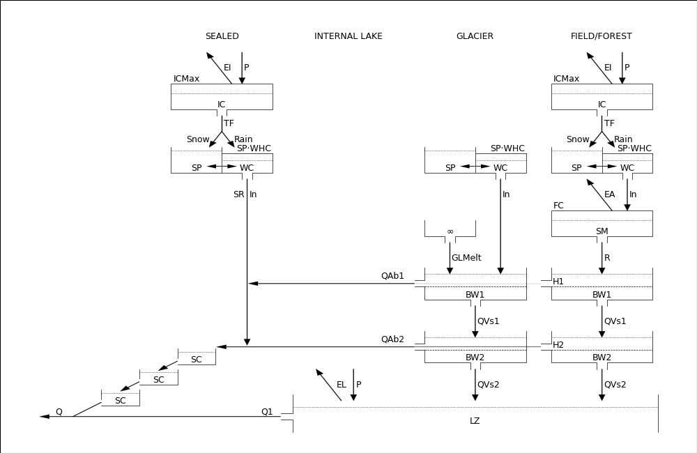
Comparing the above figure with the analogue figure of hland_v1 reveals that
hland_v4 models three instead of two runoff components, requiring a larger number of
vertically arranged storages. The two upper storages (BW1 and BW2) are
zone-specific. In comparison, the upper zone layer (UZ) of hland_v1 is
subbasin-specific. For the subbasin-wide lower zone storage (LZ), there is no
difference to hland_v1. hland_v4 allows for additional runoff concentration via a
linear storage cascade (SC), like implemented in hland_v2, which is supposed to
improve flexibility when modelling the effects of sealed areas on runoff generation.
Setting the number of storages to one agrees with COSERO’s approach to model runoff
concentration with a single bucket. In agreement with COSERO but in contrast to
hland_v2 and hland_v3, hland_v4 does not send its base flow through the storage
cascade.
Integration tests
Note
When new to HydPy, consider reading section How to understand integration tests? first.
We define the settings of the following test calculations as similar to the ones of
application model hland_v1 as possible. Hence, comparing the test results gives a
good impression of the functional differences of both models.
>>> from hydpy import pub
>>> pub.timegrids = "01.01.2000", "05.01.2000", "1h"
>>> from hydpy.models.hland_v4 import *
>>> parameterstep("1h")
>>> from hydpy import Node, Element
>>> outlet = Node("outlet")
>>> land = Element("land", outlets=outlet)
>>> land.model = model
>>> nmbzones(1)
>>> sclass(1)
>>> area(1.0)
>>> zonearea(1.0)
>>> zonez(1.0)
>>> zrelp(2.0)
>>> zrelt(2.0)
>>> zrele(2.0)
>>> psi(1.0)
>>> from hydpy import IntegrationTest
>>> IntegrationTest.plotting_options.axis1 = (
...     inputs.p, fluxes.qab1, fluxes.qab2, fluxes.q1, fluxes.rt)
>>> IntegrationTest.plotting_options.axis2 = inputs.t
>>> test = IntegrationTest(land)
>>> test.dateformat = "%d/%m %H:00"
field
We assign identical values to all parameters, besides those that are specific to
hland_v4 (H1, TAb1, TVs1, H1, TAb1, TVs1, and NmbStorages):
>>> zonetype(FIELD)
>>> pcorr(1.2)
>>> pcalt(0.1)
>>> rfcf(1.1)
>>> sfcf(1.3)
>>> tcalt(0.6)
>>> ecorr(0.8)
>>> ecalt(-0.1)
>>> epf(0.1)
>>> etf(0.1)
>>> ered(0.5)
>>> icmax(2.0)
>>> sfdist(1.0)
>>> smax(inf)
>>> sred(0.0)
>>> tt(0.0)
>>> ttint(2.0)
>>> dttm(1.0)
>>> cfmax(0.5)
>>> cfvar(0.1)
>>> gmelt(1.0)
>>> gvar(0.2)
>>> cfr(0.1)
>>> whc(0.4)
>>> fc(200.0)
>>> lp(0.8)
>>> beta(2.0)
>>> h1(10.0)
>>> tab1(2.0)
>>> tvs1(2.0)
>>> h2(10.0)
>>> tab2(10.0)
>>> tvs2(10.0)
>>> k4(0.005)
>>> gamma(0.0)
>>> maxbaz(3.0)
>>> nmbstorages(5)
>>> recstep(100)
>>> test.inits = ((states.ic, 0.0),
...               (states.sp, 0.0),
...               (states.wc, 0.0),
...               (states.sm, 100.0),
...               (states.bw1, 0.0),
...               (states.bw2, 0.0),
...               (states.lz, 10.0),
...               (states.sc, 0.05))
>>> inputs.p.series = (
...     0.0, 0.0, 0.0, 0.0, 0.0, 0.0, 0.0, 0.0, 0.0, 0.0, 0.0, 0.0, 0.0, 0.0, 0.0,
...     0.2, 0.0, 0.0, 1.3, 5.6, 2.9, 4.9, 10.6, 0.1, 0.7, 3.0, 2.1, 10.4, 3.5, 3.4,
...     1.2, 0.1, 0.0, 0.0, 0.4, 0.1, 3.6, 5.9, 1.1, 20.7, 37.9, 8.2, 3.6, 7.5, 18.5,
...     15.4, 6.3, 1.9, 4.9, 2.7, 0.5, 0.2, 0.5, 2.4, 0.4, 0.2, 0.0, 0.0, 0.3, 2.6,
...     0.7, 0.3, 0.3, 0.0, 0.0, 0.0, 0.0, 0.0, 0.0, 0.0, 0.0, 0.0, 0.0, 0.0, 0.0,
...     1.3, 0.0, 0.0, 0.0, 0.7, 0.4, 0.1, 0.4, 0.0, 0.0, 0.0, 0.0, 0.0, 0.0, 0.0,
...     0.0, 0.0, 0.0, 0.0, 0.0, 0.0)
>>> inputs.t.series = (
...     21.2, 19.4, 18.9, 18.3, 18.9, 22.5, 25.1, 28.3, 27.8, 31.4, 32.2, 35.2, 37.1,
...     31.2, 24.3, 25.4, 25.9, 23.7, 21.6, 21.2, 20.4, 19.8, 19.6, 19.2, 19.2, 19.2,
...     18.9, 18.7, 18.5, 18.3, 18.5, 18.8, 18.8, 19.0, 19.2, 19.3, 19.0, 18.8, 18.7,
...     17.8, 17.4, 17.3, 16.8, 16.5, 16.3, 16.2, 15.5, 14.6, 14.7, 14.6, 14.1, 14.3,
...     14.9, 15.7, 16.0, 16.7, 17.1, 16.2, 15.9, 16.3, 16.3, 16.4, 16.5, 18.4, 18.3,
...     18.1, 16.7, 15.2, 13.4, 12.4, 11.6, 11.0, 10.5, 11.7, 11.9, 11.2, 11.1, 11.9,
...     12.2, 11.8, 11.4, 11.6, 13.0, 17.1, 18.2, 22.4, 21.4, 21.8, 22.2, 20.1, 17.8,
...     15.2, 14.5, 12.4, 11.7, 11.9)
>>> inputs.tn.series = inputs.t.series-1.0
>>> inputs.epn.series = (
...     0.100707, 0.097801, 0.096981, 0.09599, 0.096981, 0.102761, 0.291908, 1.932875,
...     4.369536, 7.317556, 8.264362, 9.369867, 5.126178, 6.62503, 7.397619, 2.39151,
...     1.829834, 1.136569, 0.750986, 0.223895, 0.099425, 0.098454, 0.098128, 0.097474,
...     0.097474, 0.097474, 0.096981, 0.096652, 0.096321, 0.09599, 0.187298, 1.264612,
...     3.045538, 1.930758, 2.461001, 6.215945, 3.374783, 8.821555, 4.046025, 2.110757,
...     2.239257, 2.877848, 1.591452, 0.291604, 0.092622, 0.092451, 0.091248, 0.089683,
...     0.089858, 0.089683, 0.088805, 0.089157, 0.090207, 0.091593, 0.154861, 0.470369,
...     1.173726, 4.202296, 4.359715, 5.305753, 5.376027, 4.658915, 7.789594, 4.851567,
...     5.30692, 3.286036, 1.506216, 0.274762, 0.087565, 0.085771, 0.084317, 0.083215,
...     0.082289, 0.0845, 0.084864, 0.083584, 0.0834, 0.084864, 0.310229, 1.391958,
...     3.195876, 5.191651, 7.155036, 8.391432, 8.391286, 10.715238, 9.383394, 7.861915,
...     6.298329, 2.948416, 1.309232, 0.32955, 0.089508, 0.085771, 0.0845, 0.084864)
>>> test.reset_inits()
>>> conditions = sequences.conditions
hland_v4 neither implements an approach analogue to HBV96’s contributing area concept
nor a substep mechanism controlling the numerical accuracy of the runoff generation
module. Hence, we provide only a single “field” example, that is comparable both with
the first and the second example of
hland_v1:
>>> test("hland_v4_field")
Click to see the table
| date | p | t | tn | epn | tmean | tc | fracrain | rfc | sfc | cfact | swe | gact | pc | ep | epc | ei | tf | spl | wcl | spg | wcg | glmelt | melt | refr | in_ | r | sr | ea | qvs1 | qab1 | qvs2 | qab2 | el | q1 | inuh | outuh | rt | qt | ic | sp | wc | sm | bw1 | bw2 | lz | sc | outlet |
-------------------------------------------------------------------------------------------------------------------------------------------------------------------------------------------------------------------------------------------------------------------------------------------------------------------------------------------------------------------------------------------------------------------------------------------------------------------------------------------------------------
| 01/01 00:00 | 0.0 | 21.2 | 20.2 | 0.100707 | 21.8 | 21.8 | 1.0 | 1.1 | 0.0 | 0.450977 | 0.0 | 0.0 | 0.0 | 0.11682 | 0.08411 | 0.0 | 0.0 | 0.0 | 0.0 | 0.0 | 0.0 | 0.0 | 0.0 | 0.0 | 0.0 | 0.0 | 0.0 | 0.052569 | 0.0 | 0.0 | 0.0 | 0.0 | 0.0 | 0.05 | 0.0 | 0.160107 | 0.210107 | 0.058363 | 0.0 | 0.0 | 0.0 | 99.947431 | 0.0 | 0.0 | 9.95 | 0.001685 0.007302 0.016758 0.027475 0.036673 | 0.058363 |
| 01/01 01:00 | 0.0 | 19.4 | 18.4 | 0.097801 | 20.0 | 20.0 | 1.0 | 1.1 | 0.0 | 0.450977 | 0.0 | 0.0 | 0.0 | 0.113449 | 0.081683 | 0.0 | 0.0 | 0.0 | 0.0 | 0.0 | 0.0 | 0.0 | 0.0 | 0.0 | 0.0 | 0.0 | 0.0 | 0.051025 | 0.0 | 0.0 | 0.0 | 0.0 | 0.0 | 0.04975 | 0.0 | 0.073779 | 0.123529 | 0.034314 | 0.0 | 0.0 | 0.0 | 99.896406 | 0.0 | 0.0 | 9.90025 | 0.000057 0.000435 0.001704 0.004551 0.009367 | 0.034314 |
| 01/01 02:00 | 0.0 | 18.9 | 17.9 | 0.096981 | 19.5 | 19.5 | 1.0 | 1.1 | 0.0 | 0.450977 | 0.0 | 0.0 | 0.0 | 0.112498 | 0.080999 | 0.0 | 0.0 | 0.0 | 0.0 | 0.0 | 0.0 | 0.0 | 0.0 | 0.0 | 0.0 | 0.0 | 0.0 | 0.050572 | 0.0 | 0.0 | 0.0 | 0.0 | 0.0 | 0.049501 | 0.0 | 0.014282 | 0.063783 | 0.017717 | 0.0 | 0.0 | 0.0 | 99.845834 | 0.0 | 0.0 | 9.850749 | 0.000002 0.000021 0.000117 0.000439 0.001253 | 0.017717 |
| 01/01 03:00 | 0.0 | 18.3 | 17.3 | 0.09599 | 18.9 | 18.9 | 1.0 | 1.1 | 0.0 | 0.450977 | 0.0 | 0.0 | 0.0 | 0.111348 | 0.080171 | 0.0 | 0.0 | 0.0 | 0.0 | 0.0 | 0.0 | 0.0 | 0.0 | 0.0 | 0.0 | 0.0 | 0.0 | 0.05003 | 0.0 | 0.0 | 0.0 | 0.0 | 0.0 | 0.049254 | 0.0 | 0.001674 | 0.050927 | 0.014147 | 0.0 | 0.0 | 0.0 | 99.795804 | 0.0 | 0.0 | 9.801495 | 0.0 0.000001 0.000007 0.000032 0.000119 | 0.014147 |
| 01/01 04:00 | 0.0 | 18.9 | 17.9 | 0.096981 | 19.5 | 19.5 | 1.0 | 1.1 | 0.0 | 0.450977 | 0.0 | 0.0 | 0.0 | 0.112498 | 0.080999 | 0.0 | 0.0 | 0.0 | 0.0 | 0.0 | 0.0 | 0.0 | 0.0 | 0.0 | 0.0 | 0.0 | 0.0 | 0.050521 | 0.0 | 0.0 | 0.0 | 0.0 | 0.0 | 0.049007 | 0.0 | 0.000147 | 0.049155 | 0.013654 | 0.0 | 0.0 | 0.0 | 99.745284 | 0.0 | 0.0 | 9.752488 | 0.0 0.0 0.0 0.000002 0.000009 | 0.013654 |
| 01/01 05:00 | 0.0 | 22.5 | 21.5 | 0.102761 | 23.1 | 23.1 | 1.0 | 1.1 | 0.0 | 0.450977 | 0.0 | 0.0 | 0.0 | 0.119203 | 0.085826 | 0.0 | 0.0 | 0.0 | 0.0 | 0.0 | 0.0 | 0.0 | 0.0 | 0.0 | 0.0 | 0.0 | 0.0 | 0.053505 | 0.0 | 0.0 | 0.0 | 0.0 | 0.0 | 0.048762 | 0.0 | 0.000011 | 0.048773 | 0.013548 | 0.0 | 0.0 | 0.0 | 99.691779 | 0.0 | 0.0 | 9.703725 | 0.0 0.0 0.0 0.0 0.000001 | 0.013548 |
| 01/01 06:00 | 0.0 | 25.1 | 24.1 | 0.291908 | 25.7 | 25.7 | 1.0 | 1.1 | 0.0 | 0.450977 | 0.0 | 0.0 | 0.0 | 0.338613 | 0.243802 | 0.0 | 0.0 | 0.0 | 0.0 | 0.0 | 0.0 | 0.0 | 0.0 | 0.0 | 0.0 | 0.0 | 0.0 | 0.151906 | 0.0 | 0.0 | 0.0 | 0.0 | 0.0 | 0.048519 | 0.0 | 0.000001 | 0.048519 | 0.013478 | 0.0 | 0.0 | 0.0 | 99.539873 | 0.0 | 0.0 | 9.655206 | 0.0 0.0 0.0 0.0 0.0 | 0.013478 |
| 01/01 07:00 | 0.0 | 28.3 | 27.3 | 1.932875 | 28.9 | 28.9 | 1.0 | 1.1 | 0.0 | 0.450977 | 0.0 | 0.0 | 0.0 | 2.242135 | 1.614337 | 0.0 | 0.0 | 0.0 | 0.0 | 0.0 | 0.0 | 0.0 | 0.0 | 0.0 | 0.0 | 0.0 | 0.0 | 1.004318 | 0.0 | 0.0 | 0.0 | 0.0 | 0.0 | 0.048276 | 0.0 | 0.0 | 0.048276 | 0.01341 | 0.0 | 0.0 | 0.0 | 98.535555 | 0.0 | 0.0 | 9.60693 | 0.0 0.0 0.0 0.0 0.0 | 0.01341 |
| 01/01 08:00 | 0.0 | 27.8 | 26.8 | 4.369536 | 28.4 | 28.4 | 1.0 | 1.1 | 0.0 | 0.450977 | 0.0 | 0.0 | 0.0 | 5.068662 | 3.649436 | 0.0 | 0.0 | 0.0 | 0.0 | 0.0 | 0.0 | 0.0 | 0.0 | 0.0 | 0.0 | 0.0 | 0.0 | 2.247495 | 0.0 | 0.0 | 0.0 | 0.0 | 0.0 | 0.048035 | 0.0 | 0.0 | 0.048035 | 0.013343 | 0.0 | 0.0 | 0.0 | 96.288059 | 0.0 | 0.0 | 9.558896 | 0.0 0.0 0.0 0.0 0.0 | 0.013343 |
| 01/01 09:00 | 0.0 | 31.4 | 30.4 | 7.317556 | 32.0 | 32.0 | 1.0 | 1.1 | 0.0 | 0.450977 | 0.0 | 0.0 | 0.0 | 8.488365 | 6.111623 | 0.0 | 0.0 | 0.0 | 0.0 | 0.0 | 0.0 | 0.0 | 0.0 | 0.0 | 0.0 | 0.0 | 0.0 | 3.677977 | 0.0 | 0.0 | 0.0 | 0.0 | 0.0 | 0.047794 | 0.0 | 0.0 | 0.047794 | 0.013276 | 0.0 | 0.0 | 0.0 | 92.610082 | 0.0 | 0.0 | 9.511101 | 0.0 0.0 0.0 0.0 0.0 | 0.013276 |
| 01/01 10:00 | 0.0 | 32.2 | 31.2 | 8.264362 | 32.8 | 32.8 | 1.0 | 1.1 | 0.0 | 0.450977 | 0.0 | 0.0 | 0.0 | 9.58666 | 6.902395 | 0.0 | 0.0 | 0.0 | 0.0 | 0.0 | 0.0 | 0.0 | 0.0 | 0.0 | 0.0 | 0.0 | 0.0 | 3.995196 | 0.0 | 0.0 | 0.0 | 0.0 | 0.0 | 0.047556 | 0.0 | 0.0 | 0.047556 | 0.01321 | 0.0 | 0.0 | 0.0 | 88.614886 | 0.0 | 0.0 | 9.463546 | 0.0 0.0 0.0 0.0 0.0 | 0.01321 |
| 01/01 11:00 | 0.0 | 35.2 | 34.2 | 9.369867 | 35.8 | 35.8 | 1.0 | 1.1 | 0.0 | 0.450977 | 0.0 | 0.0 | 0.0 | 10.869046 | 7.825713 | 0.0 | 0.0 | 0.0 | 0.0 | 0.0 | 0.0 | 0.0 | 0.0 | 0.0 | 0.0 | 0.0 | 0.0 | 4.334217 | 0.0 | 0.0 | 0.0 | 0.0 | 0.0 | 0.047318 | 0.0 | 0.0 | 0.047318 | 0.013144 | 0.0 | 0.0 | 0.0 | 84.28067 | 0.0 | 0.0 | 9.416228 | 0.0 0.0 0.0 0.0 0.0 | 0.013144 |
| 01/01 12:00 | 0.0 | 37.1 | 36.1 | 5.126178 | 37.7 | 37.7 | 1.0 | 1.1 | 0.0 | 0.450977 | 0.0 | 0.0 | 0.0 | 5.946366 | 4.281384 | 0.0 | 0.0 | 0.0 | 0.0 | 0.0 | 0.0 | 0.0 | 0.0 | 0.0 | 0.0 | 0.0 | 0.0 | 2.255237 | 0.0 | 0.0 | 0.0 | 0.0 | 0.0 | 0.047081 | 0.0 | 0.0 | 0.047081 | 0.013078 | 0.0 | 0.0 | 0.0 | 82.025433 | 0.0 | 0.0 | 9.369147 | 0.0 0.0 0.0 0.0 0.0 | 0.013078 |
| 01/01 13:00 | 0.0 | 31.2 | 30.2 | 6.62503 | 31.8 | 31.8 | 1.0 | 1.1 | 0.0 | 0.450977 | 0.0 | 0.0 | 0.0 | 7.685035 | 5.533225 | 0.0 | 0.0 | 0.0 | 0.0 | 0.0 | 0.0 | 0.0 | 0.0 | 0.0 | 0.0 | 0.0 | 0.0 | 2.836657 | 0.0 | 0.0 | 0.0 | 0.0 | 0.0 | 0.046846 | 0.0 | 0.0 | 0.046846 | 0.013013 | 0.0 | 0.0 | 0.0 | 79.188775 | 0.0 | 0.0 | 9.322301 | 0.0 0.0 0.0 0.0 0.0 | 0.013013 |
| 01/01 14:00 | 0.0 | 24.3 | 23.3 | 7.397619 | 24.9 | 24.9 | 1.0 | 1.1 | 0.0 | 0.450977 | 0.0 | 0.0 | 0.0 | 8.581238 | 6.178491 | 0.0 | 0.0 | 0.0 | 0.0 | 0.0 | 0.0 | 0.0 | 0.0 | 0.0 | 0.0 | 0.0 | 0.0 | 3.05792 | 0.0 | 0.0 | 0.0 | 0.0 | 0.0 | 0.046612 | 0.0 | 0.0 | 0.046612 | 0.012948 | 0.0 | 0.0 | 0.0 | 76.130856 | 0.0 | 0.0 | 9.27569 | 0.0 0.0 0.0 0.0 0.0 | 0.012948 |
| 01/01 15:00 | 0.2 | 25.4 | 24.4 | 2.39151 | 26.0 | 26.0 | 1.0 | 1.1 | 0.0 | 0.450977 | 0.0 | 0.0 | 0.2376 | 2.774152 | 1.950491 | 0.2376 | 0.0 | 0.0 | 0.0 | 0.0 | 0.0 | 0.0 | 0.0 | 0.0 | 0.0 | 0.0 | 0.0 | 0.928078 | 0.0 | 0.0 | 0.0 | 0.0 | 0.0 | 0.046378 | 0.0 | 0.0 | 0.046378 | 0.012883 | 0.0 | 0.0 | 0.0 | 75.202777 | 0.0 | 0.0 | 9.229311 | 0.0 0.0 0.0 0.0 0.0 | 0.012883 |
| 01/01 16:00 | 0.0 | 25.9 | 24.9 | 1.829834 | 26.5 | 26.5 | 1.0 | 1.1 | 0.0 | 0.450977 | 0.0 | 0.0 | 0.0 | 2.122607 | 1.528277 | 0.0 | 0.0 | 0.0 | 0.0 | 0.0 | 0.0 | 0.0 | 0.0 | 0.0 | 0.0 | 0.0 | 0.0 | 0.718317 | 0.0 | 0.0 | 0.0 | 0.0 | 0.0 | 0.046147 | 0.0 | 0.0 | 0.046147 | 0.012818 | 0.0 | 0.0 | 0.0 | 74.484461 | 0.0 | 0.0 | 9.183165 | 0.0 0.0 0.0 0.0 0.0 | 0.012818 |
| 01/01 17:00 | 0.0 | 23.7 | 22.7 | 1.136569 | 24.3 | 24.3 | 1.0 | 1.1 | 0.0 | 0.450977 | 0.0 | 0.0 | 0.0 | 1.31842 | 0.949262 | 0.0 | 0.0 | 0.0 | 0.0 | 0.0 | 0.0 | 0.0 | 0.0 | 0.0 | 0.0 | 0.0 | 0.0 | 0.441908 | 0.0 | 0.0 | 0.0 | 0.0 | 0.0 | 0.045916 | 0.0 | 0.0 | 0.045916 | 0.012754 | 0.0 | 0.0 | 0.0 | 74.042552 | 0.0 | 0.0 | 9.137249 | 0.0 0.0 0.0 0.0 0.0 | 0.012754 |
| 01/01 18:00 | 1.3 | 21.6 | 20.6 | 0.750986 | 22.2 | 22.2 | 1.0 | 1.1 | 0.0 | 0.450977 | 0.0 | 0.0 | 1.5444 | 0.871144 | 0.537465 | 0.537465 | 0.0 | 0.0 | 0.0 | 0.0 | 0.0 | 0.0 | 0.0 | 0.0 | 0.0 | 0.0 | 0.0 | 0.12436 | 0.0 | 0.0 | 0.0 | 0.0 | 0.0 | 0.045686 | 0.0 | 0.0 | 0.045686 | 0.012691 | 1.006935 | 0.0 | 0.0 | 73.918192 | 0.0 | 0.0 | 9.091563 | 0.0 0.0 0.0 0.0 0.0 | 0.012691 |
| 01/01 19:00 | 5.6 | 21.2 | 20.2 | 0.223895 | 21.8 | 21.8 | 1.0 | 1.1 | 0.0 | 0.450977 | 0.0 | 0.0 | 6.6528 | 0.259718 | 0.096141 | 0.096141 | 5.659735 | 0.0 | 0.0 | 0.0 | 0.0 | 0.0 | 0.0 | 0.0 | 5.659735 | 0.773106 | 0.0 | 0.023676 | 0.164719 | 0.0 | 0.007968 | 0.0 | 0.0 | 0.045498 | 0.0 | 0.0 | 0.045498 | 0.012638 | 1.903859 | 0.0 | 0.0 | 78.781146 | 0.608387 | 0.156751 | 9.054033 | 0.0 0.0 0.0 0.0 0.0 | 0.012638 |
| 01/01 20:00 | 2.9 | 20.4 | 19.4 | 0.099425 | 21.0 | 21.0 | 1.0 | 1.1 | 0.0 | 0.450977 | 0.0 | 0.0 | 3.4452 | 0.115333 | 0.058839 | 0.058839 | 3.349059 | 0.0 | 0.0 | 0.0 | 0.0 | 0.0 | 0.0 | 0.0 | 3.349059 | 0.519646 | 0.0 | 0.015006 | 0.350098 | 0.0 | 0.031853 | 0.0 | 0.0 | 0.045429 | 0.0 | 0.0 | 0.045429 | 0.012619 | 1.941161 | 0.0 | 0.0 | 81.595554 | 0.777935 | 0.474996 | 9.040456 | 0.0 0.0 0.0 0.0 0.0 | 0.012619 |
| 01/01 21:00 | 4.9 | 19.8 | 18.8 | 0.098454 | 20.4 | 20.4 | 1.0 | 1.1 | 0.0 | 0.450977 | 0.0 | 0.0 | 5.8212 | 0.114207 | 0.045942 | 0.045942 | 5.762361 | 0.0 | 0.0 | 0.0 | 0.0 | 0.0 | 0.0 | 0.0 | 5.762361 | 0.959121 | 0.0 | 0.012404 | 0.510445 | 0.0 | 0.069894 | 0.0 | 0.0 | 0.045552 | 0.0 | 0.0 | 0.045552 | 0.012653 | 1.954058 | 0.0 | 0.0 | 86.386389 | 1.226611 | 0.915547 | 9.064799 | 0.0 0.0 0.0 0.0 0.0 | 0.012653 |
| 01/01 22:00 | 10.6 | 19.6 | 18.6 | 0.098128 | 20.2 | 20.2 | 1.0 | 1.1 | 0.0 | 0.450977 | 0.0 | 0.0 | 12.5928 | 0.113828 | 0.023264 | 0.023264 | 12.546858 | 0.0 | 0.0 | 0.0 | 0.0 | 0.0 | 0.0 | 0.0 | 12.546858 | 2.340807 | 0.0 | 0.007022 | 0.981369 | 0.0 | 0.134599 | 0.0 | 0.0 | 0.045997 | 0.0 | 0.0 | 0.045997 | 0.012777 | 1.976736 | 0.0 | 0.0 | 96.585418 | 2.586049 | 1.762317 | 9.1534 | 0.0 0.0 0.0 0.0 0.0 | 0.012777 |
| 01/01 23:00 | 0.1 | 19.2 | 18.2 | 0.097474 | 19.8 | 19.8 | 1.0 | 1.1 | 0.0 | 0.450977 | 0.0 | 0.0 | 0.1188 | 0.11307 | 0.080449 | 0.080449 | 0.095536 | 0.0 | 0.0 | 0.0 | 0.0 | 0.0 | 0.0 | 0.0 | 0.095536 | 0.022281 | 0.0 | 0.0243 | 1.022278 | 0.0 | 0.217159 | 0.0 | 0.0 | 0.046853 | 0.0 | 0.0 | 0.046853 | 0.013015 | 1.919551 | 0.0 | 0.0 | 96.634373 | 1.586051 | 2.567437 | 9.323706 | 0.0 0.0 0.0 0.0 0.0 | 0.013015 |
| 02/01 00:00 | 0.7 | 19.2 | 18.2 | 0.097474 | 19.8 | 19.8 | 1.0 | 1.1 | 0.0 | 0.451153 | 0.0 | 0.0 | 0.8316 | 0.11307 | 0.074914 | 0.074914 | 0.751151 | 0.0 | 0.0 | 0.0 | 0.0 | 0.0 | 0.0 | 0.0 | 0.751151 | 0.17536 | 0.0 | 0.022758 | 0.661425 | 0.0 | 0.27632 | 0.0 | 0.0 | 0.048 | 0.0 | 0.0 | 0.048 | 0.013333 | 1.925086 | 0.0 | 0.0 | 97.187406 | 1.099986 | 2.952542 | 9.552026 | 0.0 0.0 0.0 0.0 0.0 | 0.013333 |
| 02/01 01:00 | 3.0 | 19.2 | 18.2 | 0.097474 | 19.8 | 19.8 | 1.0 | 1.1 | 0.0 | 0.451153 | 0.0 | 0.0 | 3.564 | 0.11307 | 0.057003 | 0.057003 | 3.489086 | 0.0 | 0.0 | 0.0 | 0.0 | 0.0 | 0.0 | 0.0 | 3.489086 | 0.823895 | 0.0 | 0.017787 | 0.608351 | 0.0 | 0.3104 | 0.0 | 0.0 | 0.049312 | 0.0 | 0.0 | 0.049312 | 0.013698 | 1.942997 | 0.0 | 0.0 | 99.834811 | 1.31553 | 3.250493 | 9.813114 | 0.0 0.0 0.0 0.0 0.0 | 0.013698 |
| 02/01 02:00 | 2.1 | 18.9 | 17.9 | 0.096981 | 19.5 | 19.5 | 1.0 | 1.1 | 0.0 | 0.451153 | 0.0 | 0.0 | 2.4948 | 0.112498 | 0.063115 | 0.063115 | 2.437797 | 0.0 | 0.0 | 0.0 | 0.0 | 0.0 | 0.0 | 0.0 | 2.437797 | 0.607437 | 0.0 | 0.020052 | 0.647042 | 0.0 | 0.340625 | 0.0 | 0.0 | 0.050769 | 0.0 | 0.0 | 0.050769 | 0.014102 | 1.936885 | 0.0 | 0.0 | 101.645119 | 1.275925 | 3.55691 | 10.10297 | 0.0 0.0 0.0 0.0 0.0 | 0.014102 |
| 02/01 03:00 | 10.4 | 18.7 | 17.7 | 0.096652 | 19.3 | 19.3 | 1.0 | 1.1 | 0.0 | 0.451153 | 0.0 | 0.0 | 12.3552 | 0.112116 | 0.023465 | 0.023465 | 12.292085 | 0.0 | 0.0 | 0.0 | 0.0 | 0.0 | 0.0 | 0.0 | 12.292085 | 3.174963 | 0.0 | 0.008122 | 1.178499 | 0.0 | 0.395494 | 0.0 | 0.0 | 0.052492 | 0.0 | 0.0 | 0.052492 | 0.014581 | 1.976535 | 0.0 | 0.0 | 110.754119 | 3.272389 | 4.339915 | 10.445972 | 0.0 0.0 0.0 0.0 0.0 | 0.014581 |
| 02/01 04:00 | 3.5 | 18.5 | 17.5 | 0.096321 | 19.1 | 19.1 | 1.0 | 1.1 | 0.0 | 0.451153 | 0.0 | 0.0 | 4.158 | 0.111732 | 0.05308 | 0.05308 | 4.134535 | 0.0 | 0.0 | 0.0 | 0.0 | 0.0 | 0.0 | 0.0 | 4.134535 | 1.267904 | 0.0 | 0.018847 | 1.557726 | 0.0 | 0.488351 | 0.0 | 0.0 | 0.054672 | 0.0 | 0.0 | 0.054672 | 0.015187 | 1.94692 | 0.0 | 0.0 | 113.601903 | 2.982567 | 5.40929 | 10.879651 | 0.0 0.0 0.0 0.0 0.0 | 0.015187 |
| 02/01 05:00 | 3.4 | 18.3 | 17.3 | 0.09599 | 18.9 | 18.9 | 1.0 | 1.1 | 0.0 | 0.451153 | 0.0 | 0.0 | 4.0392 | 0.111348 | 0.05353 | 0.05353 | 3.98612 | 0.0 | 0.0 | 0.0 | 0.0 | 0.0 | 0.0 | 0.0 | 3.98612 | 1.286061 | 0.0 | 0.019455 | 1.447559 | 0.0 | 0.584786 | 0.0 | 0.0 | 0.057322 | 0.0 | 0.0 | 0.057322 | 0.015923 | 1.94647 | 0.0 | 0.0 | 116.282507 | 2.82107 | 6.272062 | 11.407116 | 0.0 0.0 0.0 0.0 0.0 | 0.015923 |
| 02/01 06:00 | 1.2 | 18.5 | 17.5 | 0.187298 | 19.1 | 19.1 | 1.0 | 1.1 | 0.0 | 0.451153 | 0.0 | 0.0 | 1.4256 | 0.217266 | 0.135647 | 0.135647 | 1.37207 | 0.0 | 0.0 | 0.0 | 0.0 | 0.0 | 0.0 | 0.0 | 1.37207 | 0.463815 | 0.0 | 0.049677 | 1.208825 | 0.0 | 0.655342 | 0.0 | 0.0 | 0.060312 | 0.0 | 0.0 | 0.060312 | 0.016753 | 1.864353 | 0.0 | 0.0 | 117.141085 | 2.076059 | 6.825546 | 12.002145 | 0.0 0.0 0.0 0.0 0.0 | 0.016753 |
| 02/01 07:00 | 0.1 | 18.8 | 17.8 | 1.264612 | 19.4 | 19.4 | 1.0 | 1.1 | 0.0 | 0.451153 | 0.0 | 0.0 | 0.1188 | 1.46695 | 1.04373 | 1.04373 | 0.0 | 0.0 | 0.0 | 0.0 | 0.0 | 0.0 | 0.0 | 0.0 | 0.0 | 0.0 | 0.0 | 0.382074 | 0.816866 | 0.0 | 0.689052 | 0.0 | 0.0 | 0.063456 | 0.0 | 0.0 | 0.063456 | 0.017627 | 0.939422 | 0.0 | 0.0 | 116.759011 | 1.259194 | 6.95336 | 12.627741 | 0.0 0.0 0.0 0.0 0.0 | 0.017627 |
| 02/01 08:00 | 0.0 | 18.8 | 17.8 | 3.045538 | 19.4 | 19.4 | 1.0 | 1.1 | 0.0 | 0.451153 | 0.0 | 0.0 | 0.0 | 3.532824 | 2.543633 | 0.939422 | 0.0 | 0.0 | 0.0 | 0.0 | 0.0 | 0.0 | 0.0 | 0.0 | 0.0 | 0.0 | 0.0 | 1.730206 | 0.495454 | 0.0 | 0.685667 | 0.0 | 0.0 | 0.066567 | 0.0 | 0.0 | 0.066567 | 0.018491 | 0.0 | 0.0 | 0.0 | 115.028805 | 0.76374 | 6.763147 | 13.246841 | 0.0 0.0 0.0 0.0 0.0 | 0.018491 |
| 02/01 09:00 | 0.0 | 19.0 | 18.0 | 1.930758 | 19.6 | 19.6 | 1.0 | 1.1 | 0.0 | 0.451153 | 0.0 | 0.0 | 0.0 | 2.239679 | 1.612569 | 0.0 | 0.0 | 0.0 | 0.0 | 0.0 | 0.0 | 0.0 | 0.0 | 0.0 | 0.0 | 0.0 | 0.0 | 1.159324 | 0.300508 | 0.0 | 0.658135 | 0.0 | 0.0 | 0.069525 | 0.0 | 0.0 | 0.069525 | 0.019312 | 0.0 | 0.0 | 0.0 | 113.869481 | 0.463231 | 6.40552 | 13.835451 | 0.0 0.0 0.0 0.0 0.0 | 0.019312 |
| 02/01 10:00 | 0.4 | 19.2 | 18.2 | 2.461001 | 19.8 | 19.8 | 1.0 | 1.1 | 0.0 | 0.451153 | 0.0 | 0.0 | 0.4752 | 2.854761 | 1.960038 | 0.4752 | 0.0 | 0.0 | 0.0 | 0.0 | 0.0 | 0.0 | 0.0 | 0.0 | 0.0 | 0.0 | 0.0 | 1.394929 | 0.182267 | 0.0 | 0.618383 | 0.0 | 0.0 | 0.072269 | 0.0 | 0.0 | 0.072269 | 0.020075 | 0.0 | 0.0 | 0.0 | 112.474552 | 0.280964 | 5.969404 | 14.381565 | 0.0 0.0 0.0 0.0 0.0 | 0.020075 |
| 02/01 11:00 | 0.1 | 19.3 | 18.3 | 6.215945 | 19.9 | 19.9 | 1.0 | 1.1 | 0.0 | 0.451153 | 0.0 | 0.0 | 0.1188 | 7.210496 | 5.130246 | 0.1188 | 0.0 | 0.0 | 0.0 | 0.0 | 0.0 | 0.0 | 0.0 | 0.0 | 0.0 | 0.0 | 0.0 | 3.606389 | 0.110551 | 0.0 | 0.573412 | 0.0 | 0.0 | 0.074775 | 0.0 | 0.0 | 0.074775 | 0.020771 | 0.0 | 0.0 | 0.0 | 108.868163 | 0.170413 | 5.506543 | 14.880202 | 0.0 0.0 0.0 0.0 0.0 | 0.020771 |
| 02/01 12:00 | 3.6 | 19.0 | 18.0 | 3.374783 | 19.6 | 19.6 | 1.0 | 1.1 | 0.0 | 0.451153 | 0.0 | 0.0 | 4.2768 | 3.914748 | 1.837796 | 1.837796 | 2.2768 | 0.0 | 0.0 | 0.0 | 0.0 | 0.0 | 0.0 | 0.0 | 2.2768 | 0.674632 | 0.0 | 0.634444 | 0.21079 | 0.0 | 0.534214 | 0.0 | 0.0 | 0.077072 | 0.0 | 0.0 | 0.077072 | 0.021409 | 0.162204 | 0.0 | 0.0 | 109.835888 | 0.634255 | 5.18312 | 15.337343 | 0.0 0.0 0.0 0.0 0.0 | 0.021409 |
| 02/01 13:00 | 5.9 | 18.8 | 17.8 | 8.821555 | 19.4 | 19.4 | 1.0 | 1.1 | 0.0 | 0.451153 | 0.0 | 0.0 | 7.0092 | 10.233004 | 3.655358 | 2.0 | 5.171404 | 0.0 | 0.0 | 0.0 | 0.0 | 0.0 | 0.0 | 0.0 | 5.171404 | 1.559685 | 0.0 | 2.12359 | 0.581868 | 0.0 | 0.521386 | 0.0 | 0.0 | 0.079294 | 0.0 | 0.0 | 0.079294 | 0.022026 | 0.0 | 0.0 | 0.0 | 111.324016 | 1.612072 | 5.243602 | 15.779436 | 0.0 0.0 0.0 0.0 0.0 | 0.022026 |
| 02/01 14:00 | 1.1 | 18.7 | 17.7 | 4.046025 | 19.3 | 19.3 | 1.0 | 1.1 | 0.0 | 0.451153 | 0.0 | 0.0 | 1.3068 | 4.693389 | 2.965278 | 1.3068 | 0.0 | 0.0 | 0.0 | 0.0 | 0.0 | 0.0 | 0.0 | 0.0 | 0.0 | 0.0 | 0.0 | 1.860822 | 0.634301 | 0.0 | 0.529678 | 0.0 | 0.0 | 0.081546 | 0.0 | 0.0 | 0.081546 | 0.022652 | 0.0 | 0.0 | 0.0 | 109.463194 | 0.977771 | 5.348224 | 16.227569 | 0.0 0.0 0.0 0.0 0.0 | 0.022652 |
| 02/01 15:00 | 20.7 | 17.8 | 16.8 | 2.110757 | 18.4 | 18.4 | 1.0 | 1.1 | 0.0 | 0.451153 | 0.0 | 0.0 | 24.5916 | 2.448478 | 0.15074 | 0.15074 | 22.5916 | 0.0 | 0.0 | 0.0 | 0.0 | 0.0 | 0.0 | 0.0 | 22.5916 | 6.767422 | 0.0 | 0.059018 | 1.826599 | 0.0 | 0.597311 | 0.0 | 0.0 | 0.084124 | 0.0 | 0.0 | 0.084124 | 0.023368 | 1.84926 | 0.0 | 0.0 | 125.228354 | 5.918594 | 6.577512 | 16.740756 | 0.0 0.0 0.0 0.0 0.0 | 0.023368 |
| 02/01 16:00 | 37.9 | 17.4 | 16.4 | 2.239257 | 18.0 | 18.0 | 1.0 | 1.1 | 0.0 | 0.451153 | 0.0 | 0.0 | 45.0252 | 2.597538 | 0.020724 | 0.020724 | 44.87446 | 0.0 | 0.0 | 0.0 | 0.0 | 0.0 | 0.0 | 0.0 | 44.87446 | 17.59319 | 0.0 | 0.009877 | 5.937839 | 1.236651 | 0.912883 | 0.026281 | 0.0 | 0.088268 | 1.262932 | 0.090148 | 0.178416 | 0.04956 | 1.979276 | 0.0 | 0.0 | 152.499747 | 16.337294 | 11.576186 | 17.56537 | 0.353906 0.31276 0.243497 0.164999 0.097622 | 0.04956 |
| 02/01 17:00 | 8.2 | 17.3 | 16.3 | 2.877848 | 17.9 | 17.9 | 1.0 | 1.1 | 0.0 | 0.451153 | 0.0 | 0.0 | 9.7416 | 3.338304 | 0.907373 | 0.907373 | 9.720876 | 0.0 | 0.0 | 0.0 | 0.0 | 0.0 | 0.0 | 0.0 | 9.720876 | 5.651759 | 0.0 | 0.443958 | 7.122851 | 2.122851 | 1.429571 | 0.429571 | 0.0 | 0.094975 | 2.552422 | 0.814543 | 0.909518 | 0.252644 | 1.092627 | 0.0 | 0.0 | 156.124906 | 12.743351 | 16.839896 | 18.899967 | 0.727183 0.682398 0.602387 0.501384 0.397312 | 0.252644 |
| 02/01 18:00 | 3.6 | 16.8 | 15.8 | 1.591452 | 17.4 | 17.4 | 1.0 | 1.1 | 0.0 | 0.451153 | 0.0 | 0.0 | 4.2768 | 1.846084 | 0.866652 | 0.866652 | 3.369427 | 0.0 | 0.0 | 0.0 | 0.0 | 0.0 | 0.0 | 0.0 | 3.369427 | 2.053243 | 0.0 | 0.426396 | 5.32071 | 0.402157 | 1.822257 | 0.822257 | 0.0 | 0.103611 | 1.224414 | 1.801219 | 1.90483 | 0.52912 | 1.133348 | 0.0 | 0.0 | 157.014694 | 9.073726 | 19.516092 | 20.618613 | 0.367621 0.407916 0.470557 0.529447 0.558317 | 0.52912 |
| 02/01 19:00 | 7.5 | 16.5 | 15.5 | 0.291604 | 17.1 | 17.1 | 1.0 | 1.1 | 0.0 | 0.451153 | 0.0 | 0.0 | 8.91 | 0.338261 | 0.099914 | 0.099914 | 8.043348 | 0.0 | 0.0 | 0.0 | 0.0 | 0.0 | 0.0 | 0.0 | 8.043348 | 4.95744 | 0.0 | 0.049957 | 4.626472 | 0.0 | 2.032304 | 1.032304 | 0.0 | 0.113255 | 1.032304 | 1.659909 | 1.773163 | 0.492545 | 1.900086 | 0.0 | 0.0 | 160.050645 | 9.404694 | 21.077957 | 22.537662 | 0.301668 0.310694 0.33024 0.361511 0.402139 | 0.492545 |
| 02/01 20:00 | 18.5 | 16.3 | 15.3 | 0.092622 | 16.9 | 16.9 | 1.0 | 1.1 | 0.0 | 0.451153 | 0.0 | 0.0 | 21.978 | 0.107442 | 0.00859 | 0.00859 | 21.878086 | 0.0 | 0.0 | 0.0 | 0.0 | 0.0 | 0.0 | 0.0 | 21.878086 | 14.01084 | 0.0 | 0.004295 | 6.466297 | 1.475918 | 2.260016 | 1.260016 | 0.0 | 0.123988 | 2.735934 | 1.332524 | 1.456512 | 0.404587 | 1.99141 | 0.0 | 0.0 | 167.913595 | 15.47332 | 24.024221 | 24.673689 | 0.776847 0.721905 0.630581 0.530141 0.450189 | 0.404587 |
| 02/01 21:00 | 15.4 | 16.2 | 15.2 | 0.092451 | 16.8 | 16.8 | 1.0 | 1.1 | 0.0 | 0.451153 | 0.0 | 0.0 | 18.2952 | 0.107243 | 0.012392 | 0.012392 | 18.28661 | 0.0 | 0.0 | 0.0 | 0.0 | 0.0 | 0.0 | 0.0 | 18.28661 | 12.889763 | 0.0 | 0.006196 | 8.18114 | 3.18114 | 2.60735 | 1.60735 | 0.0 | 0.136405 | 4.78849 | 2.181055 | 2.31746 | 0.643739 | 1.987608 | 0.0 | 0.0 | 173.304246 | 17.000803 | 27.99066 | 27.144635 | 1.368042 1.297456 1.172503 1.017338 0.86176 | 0.643739 |
| 02/01 22:00 | 6.3 | 15.5 | 14.5 | 0.091248 | 16.1 | 16.1 | 1.0 | 1.1 | 0.0 | 0.451153 | 0.0 | 0.0 | 7.4844 | 0.105848 | 0.036055 | 0.036055 | 7.472008 | 0.0 | 0.0 | 0.0 | 0.0 | 0.0 | 0.0 | 0.0 | 7.472008 | 5.610425 | 0.0 | 0.018028 | 7.324957 | 2.324957 | 2.926755 | 1.926755 | 0.0 | 0.150357 | 4.251712 | 3.733642 | 3.883999 | 1.078889 | 1.963945 | 0.0 | 0.0 | 175.147801 | 12.961313 | 30.462108 | 29.921032 | 1.237548 1.250341 1.263738 1.260066 1.223475 | 1.078889 |
| 02/01 23:00 | 1.9 | 14.6 | 13.6 | 0.089683 | 15.2 | 15.2 | 1.0 | 1.1 | 0.0 | 0.451153 | 0.0 | 0.0 | 2.2572 | 0.104032 | 0.059768 | 0.059768 | 2.221145 | 0.0 | 0.0 | 0.0 | 0.0 | 0.0 | 0.0 | 0.0 | 2.221145 | 1.703438 | 0.0 | 0.029884 | 5.324016 | 0.424173 | 3.057056 | 2.057056 | 0.0 | 0.16489 | 2.481229 | 4.168716 | 4.333607 | 1.20378 | 1.940232 | 0.0 | 0.0 | 175.635624 | 8.916561 | 30.672013 | 32.813198 | 0.737015 0.795639 0.895487 1.010309 1.109231 | 1.20378 |
| 03/01 00:00 | 4.9 | 14.7 | 13.7 | 0.089858 | 15.3 | 15.3 | 1.0 | 1.1 | 0.0 | 0.451343 | 0.0 | 0.0 | 5.8212 | 0.104235 | 0.041931 | 0.041931 | 5.761432 | 0.0 | 0.0 | 0.0 | 0.0 | 0.0 | 0.0 | 0.0 | 5.761432 | 4.443198 | 0.0 | 0.020966 | 4.455067 | 0.0 | 3.03539 | 2.03539 | 0.0 | 0.179243 | 2.03539 | 3.23013 | 3.409373 | 0.947048 | 1.958069 | 0.0 | 0.0 | 176.932892 | 8.904692 | 30.056299 | 35.669345 | 0.595209 0.613672 0.651376 0.709003 0.783681 | 0.947048 |
| 03/01 01:00 | 2.7 | 14.6 | 13.6 | 0.089683 | 15.2 | 15.2 | 1.0 | 1.1 | 0.0 | 0.451343 | 0.0 | 0.0 | 3.2076 | 0.104032 | 0.05435 | 0.05435 | 3.165669 | 0.0 | 0.0 | 0.0 | 0.0 | 0.0 | 0.0 | 0.0 | 3.165669 | 2.477551 | 0.0 | 0.027175 | 4.031594 | 0.0 | 2.959755 | 1.959755 | 0.0 | 0.193146 | 1.959755 | 2.370783 | 2.563929 | 0.712202 | 1.94565 | 0.0 | 0.0 | 177.593835 | 7.35065 | 29.168383 | 38.435955 | 0.569235 0.572877 0.581305 0.596736 0.62176 | 0.712202 |
| 03/01 02:00 | 0.5 | 14.1 | 13.1 | 0.088805 | 14.7 | 14.7 | 1.0 | 1.1 | 0.0 | 0.451343 | 0.0 | 0.0 | 0.594 | 0.103014 | 0.069893 | 0.069893 | 0.53965 | 0.0 | 0.0 | 0.0 | 0.0 | 0.0 | 0.0 | 0.0 | 0.53965 | 0.425509 | 0.0 | 0.034946 | 2.982915 | 0.0 | 2.830173 | 1.830173 | 0.0 | 0.206331 | 1.830173 | 2.037312 | 2.243642 | 0.623234 | 1.930107 | 0.0 | 0.0 | 177.673031 | 4.793244 | 27.490952 | 41.059797 | 0.532047 0.536494 0.544465 0.554869 0.5669 | 0.623234 |
| 03/01 03:00 | 0.2 | 14.3 | 13.3 | 0.089157 | 14.9 | 14.9 | 1.0 | 1.1 | 0.0 | 0.451343 | 0.0 | 0.0 | 0.2376 | 0.103422 | 0.072716 | 0.072716 | 0.167707 | 0.0 | 0.0 | 0.0 | 0.0 | 0.0 | 0.0 | 0.0 | 0.167707 | 0.132353 | 0.0 | 0.036358 | 1.914194 | 0.0 | 2.628095 | 1.628095 | 0.0 | 0.218439 | 1.628095 | 1.883328 | 2.101767 | 0.583824 | 1.927284 | 0.0 | 0.0 | 177.672027 | 3.011403 | 25.148956 | 43.469452 | 0.474166 0.481046 0.493142 0.508067 0.523121 | 0.583824 |
| 03/01 04:00 | 0.5 | 14.9 | 13.9 | 0.090207 | 15.5 | 15.5 | 1.0 | 1.1 | 0.0 | 0.451343 | 0.0 | 0.0 | 0.594 | 0.10464 | 0.070996 | 0.070996 | 0.521284 | 0.0 | 0.0 | 0.0 | 0.0 | 0.0 | 0.0 | 0.0 | 0.521284 | 0.411389 | 0.0 | 0.035498 | 1.272546 | 0.0 | 2.385782 | 1.385782 | 0.0 | 0.229276 | 1.385782 | 1.709232 | 1.938508 | 0.538475 | 1.929004 | 0.0 | 0.0 | 177.746424 | 2.150247 | 22.649937 | 45.625958 | 0.404313 0.412666 0.427518 0.446175 0.465419 | 0.538475 |
| 03/01 05:00 | 2.4 | 15.7 | 14.7 | 0.091593 | 16.3 | 16.3 | 1.0 | 1.1 | 0.0 | 0.451343 | 0.0 | 0.0 | 2.8512 | 0.106248 | 0.057521 | 0.057521 | 2.780204 | 0.0 | 0.0 | 0.0 | 0.0 | 0.0 | 0.0 | 0.0 | 2.780204 | 2.19593 | 0.0 | 0.028761 | 1.313924 | 0.0 | 2.161222 | 1.161222 | 0.0 | 0.238936 | 1.161222 | 1.49154 | 1.730476 | 0.480688 | 1.942479 | 0.0 | 0.0 | 178.301938 | 3.032252 | 20.641416 | 47.548245 | 0.339031 0.346903 0.361118 0.379475 0.399247 | 0.480688 |
| 03/01 06:00 | 0.4 | 16.0 | 15.0 | 0.154861 | 16.6 | 16.6 | 1.0 | 1.1 | 0.0 | 0.451343 | 0.0 | 0.0 | 0.4752 | 0.179639 | 0.123337 | 0.123337 | 0.417679 | 0.0 | 0.0 | 0.0 | 0.0 | 0.0 | 0.0 | 0.0 | 0.417679 | 0.331967 | 0.0 | 0.061669 | 1.263828 | 0.0 | 1.976835 | 0.976835 | 0.0 | 0.247625 | 0.976835 | 1.266305 | 1.51393 | 0.420536 | 1.876663 | 0.0 | 0.0 | 178.325981 | 2.100392 | 18.951574 | 49.277454 | 0.285161 0.29169 0.303596 0.319249 0.336609 | 0.420536 |
| 03/01 07:00 | 0.2 | 16.7 | 15.7 | 0.470369 | 17.3 | 17.3 | 1.0 | 1.1 | 0.0 | 0.451343 | 0.0 | 0.0 | 0.2376 | 0.545628 | 0.383628 | 0.383628 | 0.114263 | 0.0 | 0.0 | 0.0 | 0.0 | 0.0 | 0.0 | 0.0 | 0.114263 | 0.090839 | 0.0 | 0.191814 | 0.845794 | 0.0 | 1.804102 | 0.804102 | 0.0 | 0.255408 | 0.804102 | 1.064542 | 1.31995 | 0.366653 | 1.616372 | 0.0 | 0.0 | 178.157591 | 1.345437 | 17.189165 | 50.826148 | 0.234941 0.241 0.251963 0.266202 0.281757 | 0.366653 |
| 03/01 08:00 | 0.0 | 17.1 | 16.1 | 1.173726 | 17.7 | 17.7 | 1.0 | 1.1 | 0.0 | 0.451343 | 0.0 | 0.0 | 0.0 | 1.361522 | 0.980296 | 0.980296 | 0.0 | 0.0 | 0.0 | 0.0 | 0.0 | 0.0 | 0.0 | 0.0 | 0.0 | 0.0 | 0.0 | 0.490148 | 0.529388 | 0.0 | 1.62955 | 0.62955 | 0.0 | 0.262278 | 0.62955 | 0.883231 | 1.14551 | 0.318197 | 0.636076 | 0.0 | 0.0 | 177.667443 | 0.816049 | 15.459453 | 52.193419 | 0.184335 0.190422 0.201377 0.215459 0.230589 | 0.318197 |
| 03/01 09:00 | 0.0 | 16.2 | 15.2 | 4.202296 | 16.8 | 16.8 | 1.0 | 1.1 | 0.0 | 0.451343 | 0.0 | 0.0 | 0.0 | 4.874663 | 3.509758 | 0.636076 | 0.0 | 0.0 | 0.0 | 0.0 | 0.0 | 0.0 | 0.0 | 0.0 | 0.0 | 0.0 | 0.0 | 3.19172 | 0.32109 | 0.0 | 1.463024 | 0.463024 | 0.0 | 0.268282 | 0.463024 | 0.708663 | 0.976945 | 0.271374 | 0.0 | 0.0 | 0.0 | 174.475723 | 0.494959 | 13.854495 | 53.388162 | 0.135964 0.141793 0.152313 0.165898 0.180575 | 0.271374 |
| 03/01 10:00 | 0.3 | 15.9 | 14.9 | 4.359715 | 16.5 | 16.5 | 1.0 | 1.1 | 0.0 | 0.451343 | 0.0 | 0.0 | 0.3564 | 5.057269 | 3.513746 | 0.3564 | 0.0 | 0.0 | 0.0 | 0.0 | 0.0 | 0.0 | 0.0 | 0.0 | 0.0 | 0.0 | 0.0 | 3.335546 | 0.194751 | 0.0 | 1.311643 | 0.311643 | 0.0 | 0.273499 | 0.311643 | 0.539786 | 0.813285 | 0.225913 | 0.0 | 0.0 | 0.0 | 171.140177 | 0.300208 | 12.425959 | 54.426306 | 0.091913 0.097231 0.106862 0.119374 0.133021 | 0.225913 |
| 03/01 11:00 | 2.6 | 16.3 | 15.3 | 5.305753 | 16.9 | 16.9 | 1.0 | 1.1 | 0.0 | 0.451343 | 0.0 | 0.0 | 3.0888 | 6.154673 | 3.253813 | 2.0 | 1.0888 | 0.0 | 0.0 | 0.0 | 0.0 | 0.0 | 0.0 | 0.0 | 1.0888 | 0.797246 | 0.0 | 2.253813 | 0.287985 | 0.0 | 1.186534 | 0.186534 | 0.0 | 0.278064 | 0.186534 | 0.38314 | 0.661204 | 0.183668 | 0.0 | 0.0 | 0.0 | 169.177919 | 0.809468 | 11.340875 | 55.334776 | 0.05537 0.059797 0.067871 0.078486 0.09027 | 0.183668 |
| 03/01 12:00 | 0.7 | 16.3 | 15.3 | 5.376027 | 16.9 | 16.9 | 1.0 | 1.1 | 0.0 | 0.451343 | 0.0 | 0.0 | 0.8316 | 6.236191 | 4.131769 | 0.8316 | 0.0 | 0.0 | 0.0 | 0.0 | 0.0 | 0.0 | 0.0 | 0.0 | 0.0 | 0.0 | 0.0 | 3.715969 | 0.318501 | 0.0 | 1.089617 | 0.089617 | 0.0 | 0.282122 | 0.089617 | 0.247469 | 0.529591 | 0.147109 | 0.0 | 0.0 | 0.0 | 165.46195 | 0.490967 | 10.480141 | 56.142271 | 0.026979 0.030429 0.036755 0.045154 0.054625 | 0.147109 |
| 03/01 13:00 | 0.3 | 16.4 | 15.4 | 4.658915 | 17.0 | 17.0 | 1.0 | 1.1 | 0.0 | 0.451343 | 0.0 | 0.0 | 0.3564 | 5.404341 | 3.754888 | 0.3564 | 0.0 | 0.0 | 0.0 | 0.0 | 0.0 | 0.0 | 0.0 | 0.0 | 0.0 | 0.0 | 0.0 | 3.576688 | 0.193181 | 0.0 | 1.005627 | 0.013246 | 0.0 | 0.285739 | 0.013246 | 0.137625 | 0.423364 | 0.117601 | 0.0 | 0.0 | 0.0 | 161.885262 | 0.297787 | 9.654449 | 56.862159 | 0.004621 0.007337 0.012313 0.018919 0.026374 | 0.117601 |
| 03/01 14:00 | 0.3 | 16.5 | 15.5 | 7.789594 | 17.1 | 17.1 | 1.0 | 1.1 | 0.0 | 0.451343 | 0.0 | 0.0 | 0.3564 | 9.035929 | 6.278083 | 0.3564 | 0.0 | 0.0 | 0.0 | 0.0 | 0.0 | 0.0 | 0.0 | 0.0 | 0.0 | 0.0 | 0.0 | 6.099883 | 0.11717 | 0.0 | 0.92441 | 0.0 | 0.0 | 0.288933 | 0.0 | 0.054364 | 0.343297 | 0.09536 | 0.0 | 0.0 | 0.0 | 155.785379 | 0.180617 | 8.847209 | 57.497637 | 0.000156 0.000766 0.002113 0.004399 0.007765 | 0.09536 |
| 03/01 15:00 | 0.0 | 18.4 | 17.4 | 4.851567 | 19.0 | 19.0 | 1.0 | 1.1 | 0.0 | 0.451343 | 0.0 | 0.0 | 0.0 | 5.627818 | 4.052029 | 0.0 | 0.0 | 0.0 | 0.0 | 0.0 | 0.0 | 0.0 | 0.0 | 0.0 | 0.0 | 0.0 | 0.0 | 3.945293 | 0.071067 | 0.0 | 0.845361 | 0.0 | 0.0 | 0.291715 | 0.0 | 0.013052 | 0.304767 | 0.084657 | 0.0 | 0.0 | 0.0 | 151.840086 | 0.10955 | 8.072915 | 58.051283 | 0.000005 0.000043 0.000187 0.000564 0.001348 | 0.084657 |
| 03/01 16:00 | 0.0 | 18.3 | 17.3 | 5.30692 | 18.9 | 18.9 | 1.0 | 1.1 | 0.0 | 0.451343 | 0.0 | 0.0 | 0.0 | 6.156027 | 4.43234 | 0.0 | 0.0 | 0.0 | 0.0 | 0.0 | 0.0 | 0.0 | 0.0 | 0.0 | 0.0 | 0.0 | 0.0 | 4.206293 | 0.043104 | 0.0 | 0.770325 | 0.0 | 0.0 | 0.294108 | 0.0 | 0.00193 | 0.296038 | 0.082233 | 0.0 | 0.0 | 0.0 | 147.633793 | 0.066445 | 7.345695 | 58.527499 | 0.0 0.000002 0.000012 0.000049 0.000154 | 0.082233 |
| 03/01 17:00 | 0.0 | 18.1 | 17.1 | 3.286036 | 18.7 | 18.7 | 1.0 | 1.1 | 0.0 | 0.451343 | 0.0 | 0.0 | 0.0 | 3.811802 | 2.744497 | 0.0 | 0.0 | 0.0 | 0.0 | 0.0 | 0.0 | 0.0 | 0.0 | 0.0 | 0.0 | 0.0 | 0.0 | 2.532378 | 0.026144 | 0.0 | 0.7003 | 0.0 | 0.0 | 0.296139 | 0.0 | 0.0002 | 0.296339 | 0.082316 | 0.0 | 0.0 | 0.0 | 145.101415 | 0.040301 | 6.671539 | 58.93166 | 0.0 0.0 0.000001 0.000003 0.000014 | 0.082316 |
| 03/01 18:00 | 0.0 | 16.7 | 15.7 | 1.506216 | 17.3 | 17.3 | 1.0 | 1.1 | 0.0 | 0.451343 | 0.0 | 0.0 | 0.0 | 1.747211 | 1.257992 | 0.0 | 0.0 | 0.0 | 0.0 | 0.0 | 0.0 | 0.0 | 0.0 | 0.0 | 0.0 | 0.0 | 0.0 | 1.140852 | 0.015857 | 0.0 | 0.635648 | 0.0 | 0.0 | 0.297837 | 0.0 | 0.000016 | 0.297853 | 0.082737 | 0.0 | 0.0 | 0.0 | 143.960563 | 0.024444 | 6.051748 | 59.269472 | 0.0 0.0 0.0 0.0 0.000001 | 0.082737 |
| 03/01 19:00 | 0.0 | 15.2 | 14.2 | 0.274762 | 15.8 | 15.8 | 1.0 | 1.1 | 0.0 | 0.451343 | 0.0 | 0.0 | 0.0 | 0.318724 | 0.229481 | 0.0 | 0.0 | 0.0 | 0.0 | 0.0 | 0.0 | 0.0 | 0.0 | 0.0 | 0.0 | 0.0 | 0.0 | 0.206477 | 0.009618 | 0.0 | 0.576365 | 0.0 | 0.0 | 0.299229 | 0.0 | 0.000001 | 0.29923 | 0.08312 | 0.0 | 0.0 | 0.0 | 143.754086 | 0.014826 | 5.485001 | 59.546608 | 0.0 0.0 0.0 0.0 0.0 | 0.08312 |
| 03/01 20:00 | 0.0 | 13.4 | 12.4 | 0.087565 | 14.0 | 14.0 | 1.0 | 1.1 | 0.0 | 0.451343 | 0.0 | 0.0 | 0.0 | 0.101575 | 0.073134 | 0.0 | 0.0 | 0.0 | 0.0 | 0.0 | 0.0 | 0.0 | 0.0 | 0.0 | 0.0 | 0.0 | 0.0 | 0.065708 | 0.005834 | 0.0 | 0.522249 | 0.0 | 0.0 | 0.300344 | 0.0 | 0.0 | 0.300344 | 0.083429 | 0.0 | 0.0 | 0.0 | 143.688378 | 0.008992 | 4.968585 | 59.768512 | 0.0 0.0 0.0 0.0 0.0 | 0.083429 |
| 03/01 21:00 | 0.0 | 12.4 | 11.4 | 0.085771 | 13.0 | 13.0 | 1.0 | 1.1 | 0.0 | 0.451343 | 0.0 | 0.0 | 0.0 | 0.099494 | 0.071636 | 0.0 | 0.0 | 0.0 | 0.0 | 0.0 | 0.0 | 0.0 | 0.0 | 0.0 | 0.0 | 0.0 | 0.0 | 0.064333 | 0.003538 | 0.0 | 0.472995 | 0.0 | 0.0 | 0.301208 | 0.0 | 0.0 | 0.301208 | 0.083669 | 0.0 | 0.0 | 0.0 | 143.624045 | 0.005454 | 4.499129 | 59.9403 | 0.0 0.0 0.0 0.0 0.0 | 0.083669 |
| 03/01 22:00 | 0.0 | 11.6 | 10.6 | 0.084317 | 12.2 | 12.2 | 1.0 | 1.1 | 0.0 | 0.451343 | 0.0 | 0.0 | 0.0 | 0.097808 | 0.070422 | 0.0 | 0.0 | 0.0 | 0.0 | 0.0 | 0.0 | 0.0 | 0.0 | 0.0 | 0.0 | 0.0 | 0.0 | 0.063214 | 0.002146 | 0.0 | 0.428253 | 0.0 | 0.0 | 0.301843 | 0.0 | 0.0 | 0.301843 | 0.083845 | 0.0 | 0.0 | 0.0 | 143.560831 | 0.003308 | 4.073022 | 60.066709 | 0.0 0.0 0.0 0.0 0.0 | 0.083845 |
| 03/01 23:00 | 0.0 | 11.0 | 10.0 | 0.083215 | 11.6 | 11.6 | 1.0 | 1.1 | 0.0 | 0.451343 | 0.0 | 0.0 | 0.0 | 0.096529 | 0.069501 | 0.0 | 0.0 | 0.0 | 0.0 | 0.0 | 0.0 | 0.0 | 0.0 | 0.0 | 0.0 | 0.0 | 0.0 | 0.06236 | 0.001302 | 0.0 | 0.387662 | 0.0 | 0.0 | 0.302272 | 0.0 | 0.0 | 0.302272 | 0.083964 | 0.0 | 0.0 | 0.0 | 143.498471 | 0.002006 | 3.686662 | 60.1521 | 0.0 0.0 0.0 0.0 0.0 | 0.083964 |
| 04/01 00:00 | 0.0 | 10.5 | 9.5 | 0.082289 | 11.1 | 11.1 | 1.0 | 1.1 | 0.0 | 0.451548 | 0.0 | 0.0 | 0.0 | 0.095455 | 0.068728 | 0.0 | 0.0 | 0.0 | 0.0 | 0.0 | 0.0 | 0.0 | 0.0 | 0.0 | 0.0 | 0.0 | 0.0 | 0.06164 | 0.000789 | 0.0 | 0.35087 | 0.0 | 0.0 | 0.302515 | 0.0 | 0.0 | 0.302515 | 0.084032 | 0.0 | 0.0 | 0.0 | 143.436831 | 0.001217 | 3.336581 | 60.200455 | 0.0 0.0 0.0 0.0 0.0 | 0.084032 |
| 04/01 01:00 | 0.0 | 11.7 | 10.7 | 0.0845 | 12.3 | 12.3 | 1.0 | 1.1 | 0.0 | 0.451548 | 0.0 | 0.0 | 0.0 | 0.09802 | 0.070574 | 0.0 | 0.0 | 0.0 | 0.0 | 0.0 | 0.0 | 0.0 | 0.0 | 0.0 | 0.0 | 0.0 | 0.0 | 0.063269 | 0.000479 | 0.0 | 0.317541 | 0.0 | 0.0 | 0.30259 | 0.0 | 0.0 | 0.30259 | 0.084053 | 0.0 | 0.0 | 0.0 | 143.373563 | 0.000738 | 3.019519 | 60.215406 | 0.0 0.0 0.0 0.0 0.0 | 0.084053 |
| 04/01 02:00 | 0.0 | 11.9 | 10.9 | 0.084864 | 12.5 | 12.5 | 1.0 | 1.1 | 0.0 | 0.451548 | 0.0 | 0.0 | 0.0 | 0.098442 | 0.070878 | 0.0 | 0.0 | 0.0 | 0.0 | 0.0 | 0.0 | 0.0 | 0.0 | 0.0 | 0.0 | 0.0 | 0.0 | 0.063513 | 0.00029 | 0.0 | 0.287359 | 0.0 | 0.0 | 0.302514 | 0.0 | 0.0 | 0.302514 | 0.084032 | 0.0 | 0.0 | 0.0 | 143.31005 | 0.000448 | 2.73245 | 60.200252 | 0.0 0.0 0.0 0.0 0.0 | 0.084032 |
| 04/01 03:00 | 1.3 | 11.2 | 10.2 | 0.083584 | 11.8 | 11.8 | 1.0 | 1.1 | 0.0 | 0.451548 | 0.0 | 0.0 | 1.5444 | 0.096957 | 0.059819 | 0.059819 | 0.0 | 0.0 | 0.0 | 0.0 | 0.0 | 0.0 | 0.0 | 0.0 | 0.0 | 0.0 | 0.0 | 0.02679 | 0.000176 | 0.0 | 0.260036 | 0.0 | 0.0 | 0.302301 | 0.0 | 0.0 | 0.302301 | 0.083973 | 1.484581 | 0.0 | 0.0 | 143.28326 | 0.000272 | 2.472591 | 60.157986 | 0.0 0.0 0.0 0.0 0.0 | 0.083973 |
| 04/01 04:00 | 0.0 | 11.1 | 10.1 | 0.0834 | 11.7 | 11.7 | 1.0 | 1.1 | 0.0 | 0.451548 | 0.0 | 0.0 | 0.0 | 0.096744 | 0.069656 | 0.069656 | 0.0 | 0.0 | 0.0 | 0.0 | 0.0 | 0.0 | 0.0 | 0.0 | 0.0 | 0.0 | 0.0 | 0.031189 | 0.000107 | 0.0 | 0.235303 | 0.0 | 0.0 | 0.301966 | 0.0 | 0.0 | 0.301966 | 0.08388 | 1.414925 | 0.0 | 0.0 | 143.252071 | 0.000165 | 2.237394 | 60.091323 | 0.0 0.0 0.0 0.0 0.0 | 0.08388 |
| 04/01 05:00 | 0.0 | 11.9 | 10.9 | 0.084864 | 12.5 | 12.5 | 1.0 | 1.1 | 0.0 | 0.451548 | 0.0 | 0.0 | 0.0 | 0.098442 | 0.070878 | 0.070878 | 0.0 | 0.0 | 0.0 | 0.0 | 0.0 | 0.0 | 0.0 | 0.0 | 0.0 | 0.0 | 0.0 | 0.03173 | 0.000065 | 0.0 | 0.212919 | 0.0 | 0.0 | 0.301521 | 0.0 | 0.0 | 0.301521 | 0.083756 | 1.344047 | 0.0 | 0.0 | 143.220341 | 0.0001 | 2.02454 | 60.002721 | 0.0 0.0 0.0 0.0 0.0 | 0.083756 |
| 04/01 06:00 | 0.0 | 12.2 | 11.2 | 0.310229 | 12.8 | 12.8 | 1.0 | 1.1 | 0.0 | 0.451548 | 0.0 | 0.0 | 0.0 | 0.359866 | 0.259103 | 0.259103 | 0.0 | 0.0 | 0.0 | 0.0 | 0.0 | 0.0 | 0.0 | 0.0 | 0.0 | 0.0 | 0.0 | 0.115965 | 0.000039 | 0.0 | 0.192662 | 0.0 | 0.0 | 0.300977 | 0.0 | 0.0 | 0.300977 | 0.083605 | 1.084943 | 0.0 | 0.0 | 143.104376 | 0.000061 | 1.831917 | 59.894406 | 0.0 0.0 0.0 0.0 0.0 | 0.083605 |
| 04/01 07:00 | 0.7 | 11.8 | 10.8 | 1.391958 | 12.4 | 12.4 | 1.0 | 1.1 | 0.0 | 0.451548 | 0.0 | 0.0 | 0.8316 | 1.614671 | 1.069795 | 1.069795 | 0.0 | 0.0 | 0.0 | 0.0 | 0.0 | 0.0 | 0.0 | 0.0 | 0.0 | 0.0 | 0.0 | 0.478414 | 0.000024 | 0.0 | 0.174331 | 0.0 | 0.0 | 0.300344 | 0.0 | 0.0 | 0.300344 | 0.083429 | 0.846748 | 0.0 | 0.0 | 142.625962 | 0.000037 | 1.657609 | 59.768393 | 0.0 0.0 0.0 0.0 0.0 | 0.083429 |
| 04/01 08:00 | 0.4 | 11.4 | 10.4 | 3.195876 | 12.0 | 12.0 | 1.0 | 1.1 | 0.0 | 0.451548 | 0.0 | 0.0 | 0.4752 | 3.707216 | 2.545322 | 1.321948 | 0.0 | 0.0 | 0.0 | 0.0 | 0.0 | 0.0 | 0.0 | 0.0 | 0.0 | 0.0 | 0.0 | 1.746153 | 0.000014 | 0.0 | 0.157743 | 0.0 | 0.0 | 0.299631 | 0.0 | 0.0 | 0.299631 | 0.083231 | 0.0 | 0.0 | 0.0 | 140.87981 | 0.000022 | 1.499881 | 59.626506 | 0.0 0.0 0.0 0.0 0.0 | 0.083231 |
| 04/01 09:00 | 0.1 | 11.6 | 10.6 | 5.191651 | 12.2 | 12.2 | 1.0 | 1.1 | 0.0 | 0.451548 | 0.0 | 0.0 | 0.1188 | 6.022315 | 4.284859 | 0.1188 | 0.0 | 0.0 | 0.0 | 0.0 | 0.0 | 0.0 | 0.0 | 0.0 | 0.0 | 0.0 | 0.0 | 3.772813 | 0.000009 | 0.0 | 0.142733 | 0.0 | 0.0 | 0.298846 | 0.0 | 0.0 | 0.298846 | 0.083013 | 0.0 | 0.0 | 0.0 | 137.106996 | 0.000014 | 1.357157 | 59.470393 | 0.0 0.0 0.0 0.0 0.0 | 0.083013 |
| 04/01 10:00 | 0.4 | 13.0 | 12.0 | 7.155036 | 13.6 | 13.6 | 1.0 | 1.1 | 0.0 | 0.451548 | 0.0 | 0.0 | 0.4752 | 8.299842 | 5.698554 | 0.4752 | 0.0 | 0.0 | 0.0 | 0.0 | 0.0 | 0.0 | 0.0 | 0.0 | 0.0 | 0.0 | 0.0 | 4.883197 | 0.000005 | 0.0 | 0.129151 | 0.0 | 0.0 | 0.297998 | 0.0 | 0.0 | 0.297998 | 0.082777 | 0.0 | 0.0 | 0.0 | 132.223799 | 0.000008 | 1.228011 | 59.301546 | 0.0 0.0 0.0 0.0 0.0 | 0.082777 |
| 04/01 11:00 | 0.0 | 17.1 | 16.1 | 8.391432 | 17.7 | 17.7 | 1.0 | 1.1 | 0.0 | 0.451548 | 0.0 | 0.0 | 0.0 | 9.734061 | 7.008524 | 0.0 | 0.0 | 0.0 | 0.0 | 0.0 | 0.0 | 0.0 | 0.0 | 0.0 | 0.0 | 0.0 | 0.0 | 5.791835 | 0.000003 | 0.0 | 0.116861 | 0.0 | 0.0 | 0.297092 | 0.0 | 0.0 | 0.297092 | 0.082526 | 0.0 | 0.0 | 0.0 | 126.431964 | 0.000005 | 1.111154 | 59.121315 | 0.0 0.0 0.0 0.0 0.0 | 0.082526 |
| 04/01 12:00 | 0.0 | 18.2 | 17.2 | 8.391286 | 18.8 | 18.8 | 1.0 | 1.1 | 0.0 | 0.451548 | 0.0 | 0.0 | 0.0 | 9.733892 | 7.008402 | 0.0 | 0.0 | 0.0 | 0.0 | 0.0 | 0.0 | 0.0 | 0.0 | 0.0 | 0.0 | 0.0 | 0.0 | 5.538038 | 0.000002 | 0.0 | 0.10574 | 0.0 | 0.0 | 0.296135 | 0.0 | 0.0 | 0.296135 | 0.08226 | 0.0 | 0.0 | 0.0 | 120.893926 | 0.000003 | 1.005415 | 58.93092 | 0.0 0.0 0.0 0.0 0.0 | 0.08226 |
| 04/01 13:00 | 0.0 | 22.4 | 21.4 | 10.715238 | 23.0 | 23.0 | 1.0 | 1.1 | 0.0 | 0.451548 | 0.0 | 0.0 | 0.0 | 12.429676 | 8.949367 | 0.0 | 0.0 | 0.0 | 0.0 | 0.0 | 0.0 | 0.0 | 0.0 | 0.0 | 0.0 | 0.0 | 0.0 | 6.762026 | 0.000001 | 0.0 | 0.095678 | 0.0 | 0.0 | 0.295133 | 0.0 | 0.0 | 0.295133 | 0.081981 | 0.0 | 0.0 | 0.0 | 114.1319 | 0.000002 | 0.909738 | 58.731465 | 0.0 0.0 0.0 0.0 0.0 | 0.081981 |
| 04/01 14:00 | 0.0 | 21.4 | 20.4 | 9.383394 | 22.0 | 22.0 | 1.0 | 1.1 | 0.0 | 0.451548 | 0.0 | 0.0 | 0.0 | 10.884737 | 7.837011 | 0.0 | 0.0 | 0.0 | 0.0 | 0.0 | 0.0 | 0.0 | 0.0 | 0.0 | 0.0 | 0.0 | 0.0 | 5.590331 | 0.000001 | 0.0 | 0.086573 | 0.0 | 0.0 | 0.29409 | 0.0 | 0.0 | 0.29409 | 0.081692 | 0.0 | 0.0 | 0.0 | 108.54157 | 0.000001 | 0.823166 | 58.523947 | 0.0 0.0 0.0 0.0 0.0 | 0.081692 |
| 04/01 15:00 | 0.0 | 21.8 | 20.8 | 7.861915 | 22.4 | 22.4 | 1.0 | 1.1 | 0.0 | 0.451548 | 0.0 | 0.0 | 0.0 | 9.119821 | 6.566271 | 0.0 | 0.0 | 0.0 | 0.0 | 0.0 | 0.0 | 0.0 | 0.0 | 0.0 | 0.0 | 0.0 | 0.0 | 4.454459 | 0.0 | 0.0 | 0.078335 | 0.0 | 0.0 | 0.293011 | 0.0 | 0.0 | 0.293011 | 0.081392 | 0.0 | 0.0 | 0.0 | 104.087111 | 0.000001 | 0.744832 | 58.309271 | 0.0 0.0 0.0 0.0 0.0 | 0.081392 |
| 04/01 16:00 | 0.0 | 22.2 | 21.2 | 6.298329 | 22.8 | 22.8 | 1.0 | 1.1 | 0.0 | 0.451548 | 0.0 | 0.0 | 0.0 | 7.306062 | 5.260364 | 0.0 | 0.0 | 0.0 | 0.0 | 0.0 | 0.0 | 0.0 | 0.0 | 0.0 | 0.0 | 0.0 | 0.0 | 3.422101 | 0.0 | 0.0 | 0.07088 | 0.0 | 0.0 | 0.291901 | 0.0 | 0.0 | 0.291901 | 0.081084 | 0.0 | 0.0 | 0.0 | 100.66501 | 0.0 | 0.673952 | 58.08825 | 0.0 0.0 0.0 0.0 0.0 | 0.081084 |
| 04/01 17:00 | 0.0 | 20.1 | 19.1 | 2.948416 | 20.7 | 20.7 | 1.0 | 1.1 | 0.0 | 0.451548 | 0.0 | 0.0 | 0.0 | 3.420163 | 2.462517 | 0.0 | 0.0 | 0.0 | 0.0 | 0.0 | 0.0 | 0.0 | 0.0 | 0.0 | 0.0 | 0.0 | 0.0 | 1.549308 | 0.0 | 0.0 | 0.064135 | 0.0 | 0.0 | 0.290762 | 0.0 | 0.0 | 0.290762 | 0.080767 | 0.0 | 0.0 | 0.0 | 99.115702 | 0.0 | 0.609817 | 57.861623 | 0.0 0.0 0.0 0.0 0.0 | 0.080767 |
| 04/01 18:00 | 0.0 | 17.8 | 16.8 | 1.309232 | 18.4 | 18.4 | 1.0 | 1.1 | 0.0 | 0.451548 | 0.0 | 0.0 | 0.0 | 1.518709 | 1.093471 | 0.0 | 0.0 | 0.0 | 0.0 | 0.0 | 0.0 | 0.0 | 0.0 | 0.0 | 0.0 | 0.0 | 0.0 | 0.677376 | 0.0 | 0.0 | 0.058032 | 0.0 | 0.0 | 0.289598 | 0.0 | 0.0 | 0.289598 | 0.080444 | 0.0 | 0.0 | 0.0 | 98.438326 | 0.0 | 0.551785 | 57.630057 | 0.0 0.0 0.0 0.0 0.0 | 0.080444 |
| 04/01 19:00 | 0.0 | 15.2 | 14.2 | 0.32955 | 15.8 | 15.8 | 1.0 | 1.1 | 0.0 | 0.451548 | 0.0 | 0.0 | 0.0 | 0.382278 | 0.27524 | 0.0 | 0.0 | 0.0 | 0.0 | 0.0 | 0.0 | 0.0 | 0.0 | 0.0 | 0.0 | 0.0 | 0.0 | 0.169339 | 0.0 | 0.0 | 0.052509 | 0.0 | 0.0 | 0.288413 | 0.0 | 0.0 | 0.288413 | 0.080115 | 0.0 | 0.0 | 0.0 | 98.268988 | 0.0 | 0.499276 | 57.394153 | 0.0 0.0 0.0 0.0 0.0 | 0.080115 |
| 04/01 20:00 | 0.0 | 14.5 | 13.5 | 0.089508 | 15.1 | 15.1 | 1.0 | 1.1 | 0.0 | 0.451548 | 0.0 | 0.0 | 0.0 | 0.103829 | 0.074757 | 0.0 | 0.0 | 0.0 | 0.0 | 0.0 | 0.0 | 0.0 | 0.0 | 0.0 | 0.0 | 0.0 | 0.0 | 0.045914 | 0.0 | 0.0 | 0.047512 | 0.0 | 0.0 | 0.287208 | 0.0 | 0.0 | 0.287208 | 0.07978 | 0.0 | 0.0 | 0.0 | 98.223073 | 0.0 | 0.451764 | 57.154457 | 0.0 0.0 0.0 0.0 0.0 | 0.07978 |
| 04/01 21:00 | 0.0 | 12.4 | 11.4 | 0.085771 | 13.0 | 13.0 | 1.0 | 1.1 | 0.0 | 0.451548 | 0.0 | 0.0 | 0.0 | 0.099494 | 0.071636 | 0.0 | 0.0 | 0.0 | 0.0 | 0.0 | 0.0 | 0.0 | 0.0 | 0.0 | 0.0 | 0.0 | 0.0 | 0.043977 | 0.0 | 0.0 | 0.042991 | 0.0 | 0.0 | 0.285987 | 0.0 | 0.0 | 0.285987 | 0.079441 | 0.0 | 0.0 | 0.0 | 98.179096 | 0.0 | 0.408773 | 56.911461 | 0.0 0.0 0.0 0.0 0.0 | 0.079441 |
| 04/01 22:00 | 0.0 | 11.7 | 10.7 | 0.0845 | 12.3 | 12.3 | 1.0 | 1.1 | 0.0 | 0.451548 | 0.0 | 0.0 | 0.0 | 0.09802 | 0.070574 | 0.0 | 0.0 | 0.0 | 0.0 | 0.0 | 0.0 | 0.0 | 0.0 | 0.0 | 0.0 | 0.0 | 0.0 | 0.043306 | 0.0 | 0.0 | 0.0389 | 0.0 | 0.0 | 0.284752 | 0.0 | 0.0 | 0.284752 | 0.079098 | 0.0 | 0.0 | 0.0 | 98.13579 | 0.0 | 0.369873 | 56.665609 | 0.0 0.0 0.0 0.0 0.0 | 0.079098 |
| 04/01 23:00 | 0.0 | 11.9 | 10.9 | 0.084864 | 12.5 | 12.5 | 1.0 | 1.1 | 0.0 | 0.451548 | 0.0 | 0.0 | 0.0 | 0.098442 | 0.070878 | 0.0 | 0.0 | 0.0 | 0.0 | 0.0 | 0.0 | 0.0 | 0.0 | 0.0 | 0.0 | 0.0 | 0.0 | 0.043473 | 0.0 | 0.0 | 0.035198 | 0.0 | 0.0 | 0.283504 | 0.0 | 0.0 | 0.283504 | 0.078751 | 0.0 | 0.0 | 0.0 | 98.092317 | 0.0 | 0.334675 | 56.417303 | 0.0 0.0 0.0 0.0 0.0 | 0.078751 |
Click to see the graphThere is no indication of an error in the water balance:
>>> from hydpy import round_
>>> round_(model.check_waterbalance(conditions))
0.0
Regarding numerical accuracy of the linear storage cascade, please see the
low accuracy example of hland_v2, which also applies the storage
cascade instead of the triangular Unit Hydrograph.
internal lake
Regarding the simulation of internal lakes, the functionalities of hland_v4 are
identical to hland_v1. Hence, the simulated baseflow shown in the following table
agrees with the internal lake example of hland_v1. Nevertheless, the
resulting subbasin’s outflow appears less smoothed due to hland_v4 not sending its
baseflow through the linear storage cascade:
>>> recstep(100)
>>> zonetype(ILAKE)
>>> ttice(13.0)
>>> test.inits.sc = 0.0
>>> test.reset_inits()
>>> conditions = sequences.conditions
>>> test("hland_v4_ilake")
Click to see the table
| date | p | t | tn | epn | tmean | tc | fracrain | rfc | sfc | cfact | swe | gact | pc | ep | epc | ei | tf | spl | wcl | spg | wcg | glmelt | melt | refr | in_ | r | sr | ea | qvs1 | qab1 | qvs2 | qab2 | el | q1 | inuh | outuh | rt | qt | ic | sp | wc | sm | bw1 | bw2 | lz | sc | outlet |
------------------------------------------------------------------------------------------------------------------------------------------------------------------------------------------------------------------------------------------------------------------------------------------------------------------------------------------------------------------------------------------------------------------------
| 01/01 00:00 | 0.0 | 21.2 | 20.2 | 0.100707 | 21.8 | 21.8 | 1.0 | 1.1 | 0.0 | 0.0 | 0.0 | 0.0 | 0.0 | 0.11682 | 0.08411 | 0.0 | 0.0 | 0.0 | 0.0 | 0.0 | 0.0 | 0.0 | 0.0 | 0.0 | 0.0 | 0.0 | 0.0 | 0.0 | 0.0 | 0.0 | 0.0 | 0.0 | 0.08411 | 0.049579 | 0.0 | 0.0 | 0.049579 | 0.013772 | 0.0 | 0.0 | 0.0 | 0.0 | 0.0 | 0.0 | 9.86631 | 0.0 0.0 0.0 0.0 0.0 | 0.013772 |
| 01/01 01:00 | 0.0 | 19.4 | 18.4 | 0.097801 | 20.0 | 20.0 | 1.0 | 1.1 | 0.0 | 0.0 | 0.0 | 0.0 | 0.0 | 0.113449 | 0.081683 | 0.0 | 0.0 | 0.0 | 0.0 | 0.0 | 0.0 | 0.0 | 0.0 | 0.0 | 0.0 | 0.0 | 0.0 | 0.0 | 0.0 | 0.0 | 0.0 | 0.0 | 0.081683 | 0.048923 | 0.0 | 0.0 | 0.048923 | 0.01359 | 0.0 | 0.0 | 0.0 | 0.0 | 0.0 | 0.0 | 9.735704 | 0.0 0.0 0.0 0.0 0.0 | 0.01359 |
| 01/01 02:00 | 0.0 | 18.9 | 17.9 | 0.096981 | 19.5 | 19.5 | 1.0 | 1.1 | 0.0 | 0.0 | 0.0 | 0.0 | 0.0 | 0.112498 | 0.080999 | 0.0 | 0.0 | 0.0 | 0.0 | 0.0 | 0.0 | 0.0 | 0.0 | 0.0 | 0.0 | 0.0 | 0.0 | 0.0 | 0.0 | 0.0 | 0.0 | 0.0 | 0.080999 | 0.048274 | 0.0 | 0.0 | 0.048274 | 0.013409 | 0.0 | 0.0 | 0.0 | 0.0 | 0.0 | 0.0 | 9.606431 | 0.0 0.0 0.0 0.0 0.0 | 0.013409 |
| 01/01 03:00 | 0.0 | 18.3 | 17.3 | 0.09599 | 18.9 | 18.9 | 1.0 | 1.1 | 0.0 | 0.0 | 0.0 | 0.0 | 0.0 | 0.111348 | 0.080171 | 0.0 | 0.0 | 0.0 | 0.0 | 0.0 | 0.0 | 0.0 | 0.0 | 0.0 | 0.0 | 0.0 | 0.0 | 0.0 | 0.0 | 0.0 | 0.0 | 0.0 | 0.080171 | 0.047631 | 0.0 | 0.0 | 0.047631 | 0.013231 | 0.0 | 0.0 | 0.0 | 0.0 | 0.0 | 0.0 | 9.478629 | 0.0 0.0 0.0 0.0 0.0 | 0.013231 |
| 01/01 04:00 | 0.0 | 18.9 | 17.9 | 0.096981 | 19.5 | 19.5 | 1.0 | 1.1 | 0.0 | 0.0 | 0.0 | 0.0 | 0.0 | 0.112498 | 0.080999 | 0.0 | 0.0 | 0.0 | 0.0 | 0.0 | 0.0 | 0.0 | 0.0 | 0.0 | 0.0 | 0.0 | 0.0 | 0.0 | 0.0 | 0.0 | 0.0 | 0.0 | 0.080999 | 0.046988 | 0.0 | 0.0 | 0.046988 | 0.013052 | 0.0 | 0.0 | 0.0 | 0.0 | 0.0 | 0.0 | 9.350643 | 0.0 0.0 0.0 0.0 0.0 | 0.013052 |
| 01/01 05:00 | 0.0 | 22.5 | 21.5 | 0.102761 | 23.1 | 23.1 | 1.0 | 1.1 | 0.0 | 0.0 | 0.0 | 0.0 | 0.0 | 0.119203 | 0.085826 | 0.0 | 0.0 | 0.0 | 0.0 | 0.0 | 0.0 | 0.0 | 0.0 | 0.0 | 0.0 | 0.0 | 0.0 | 0.0 | 0.0 | 0.0 | 0.0 | 0.0 | 0.085826 | 0.046324 | 0.0 | 0.0 | 0.046324 | 0.012868 | 0.0 | 0.0 | 0.0 | 0.0 | 0.0 | 0.0 | 9.218493 | 0.0 0.0 0.0 0.0 0.0 | 0.012868 |
| 01/01 06:00 | 0.0 | 25.1 | 24.1 | 0.291908 | 25.7 | 25.7 | 1.0 | 1.1 | 0.0 | 0.0 | 0.0 | 0.0 | 0.0 | 0.338613 | 0.243802 | 0.0 | 0.0 | 0.0 | 0.0 | 0.0 | 0.0 | 0.0 | 0.0 | 0.0 | 0.0 | 0.0 | 0.0 | 0.0 | 0.0 | 0.0 | 0.0 | 0.0 | 0.243802 | 0.044873 | 0.0 | 0.0 | 0.044873 | 0.012465 | 0.0 | 0.0 | 0.0 | 0.0 | 0.0 | 0.0 | 8.929818 | 0.0 0.0 0.0 0.0 0.0 | 0.012465 |
| 01/01 07:00 | 0.0 | 28.3 | 27.3 | 1.932875 | 28.9 | 28.9 | 1.0 | 1.1 | 0.0 | 0.0 | 0.0 | 0.0 | 0.0 | 2.242135 | 1.614337 | 0.0 | 0.0 | 0.0 | 0.0 | 0.0 | 0.0 | 0.0 | 0.0 | 0.0 | 0.0 | 0.0 | 0.0 | 0.0 | 0.0 | 0.0 | 0.0 | 0.0 | 1.614337 | 0.036577 | 0.0 | 0.0 | 0.036577 | 0.01016 | 0.0 | 0.0 | 0.0 | 0.0 | 0.0 | 0.0 | 7.278903 | 0.0 0.0 0.0 0.0 0.0 | 0.01016 |
| 01/01 08:00 | 0.0 | 27.8 | 26.8 | 4.369536 | 28.4 | 28.4 | 1.0 | 1.1 | 0.0 | 0.0 | 0.0 | 0.0 | 0.0 | 5.068662 | 3.649436 | 0.0 | 0.0 | 0.0 | 0.0 | 0.0 | 0.0 | 0.0 | 0.0 | 0.0 | 0.0 | 0.0 | 0.0 | 0.0 | 0.0 | 0.0 | 0.0 | 0.0 | 3.649436 | 0.018147 | 0.0 | 0.0 | 0.018147 | 0.005041 | 0.0 | 0.0 | 0.0 | 0.0 | 0.0 | 0.0 | 3.611319 | 0.0 0.0 0.0 0.0 0.0 | 0.005041 |
| 01/01 09:00 | 0.0 | 31.4 | 30.4 | 7.317556 | 32.0 | 32.0 | 1.0 | 1.1 | 0.0 | 0.0 | 0.0 | 0.0 | 0.0 | 8.488365 | 6.111623 | 0.0 | 0.0 | 0.0 | 0.0 | 0.0 | 0.0 | 0.0 | 0.0 | 0.0 | 0.0 | 0.0 | 0.0 | 0.0 | 0.0 | 0.0 | 0.0 | 0.0 | 6.111623 | 0.0 | 0.0 | 0.0 | 0.0 | 0.0 | 0.0 | 0.0 | 0.0 | 0.0 | 0.0 | 0.0 | -2.500304 | 0.0 0.0 0.0 0.0 0.0 | 0.0 |
| 01/01 10:00 | 0.0 | 32.2 | 31.2 | 8.264362 | 32.8 | 32.8 | 1.0 | 1.1 | 0.0 | 0.0 | 0.0 | 0.0 | 0.0 | 9.58666 | 6.902395 | 0.0 | 0.0 | 0.0 | 0.0 | 0.0 | 0.0 | 0.0 | 0.0 | 0.0 | 0.0 | 0.0 | 0.0 | 0.0 | 0.0 | 0.0 | 0.0 | 0.0 | 6.902395 | 0.0 | 0.0 | 0.0 | 0.0 | 0.0 | 0.0 | 0.0 | 0.0 | 0.0 | 0.0 | 0.0 | -9.402699 | 0.0 0.0 0.0 0.0 0.0 | 0.0 |
| 01/01 11:00 | 0.0 | 35.2 | 34.2 | 9.369867 | 35.8 | 35.8 | 1.0 | 1.1 | 0.0 | 0.0 | 0.0 | 0.0 | 0.0 | 10.869046 | 7.825713 | 0.0 | 0.0 | 0.0 | 0.0 | 0.0 | 0.0 | 0.0 | 0.0 | 0.0 | 0.0 | 0.0 | 0.0 | 0.0 | 0.0 | 0.0 | 0.0 | 0.0 | 7.825713 | 0.0 | 0.0 | 0.0 | 0.0 | 0.0 | 0.0 | 0.0 | 0.0 | 0.0 | 0.0 | 0.0 | -17.228412 | 0.0 0.0 0.0 0.0 0.0 | 0.0 |
| 01/01 12:00 | 0.0 | 37.1 | 36.1 | 5.126178 | 37.7 | 37.7 | 1.0 | 1.1 | 0.0 | 0.0 | 0.0 | 0.0 | 0.0 | 5.946366 | 4.281384 | 0.0 | 0.0 | 0.0 | 0.0 | 0.0 | 0.0 | 0.0 | 0.0 | 0.0 | 0.0 | 0.0 | 0.0 | 0.0 | 0.0 | 0.0 | 0.0 | 0.0 | 4.281384 | 0.0 | 0.0 | 0.0 | 0.0 | 0.0 | 0.0 | 0.0 | 0.0 | 0.0 | 0.0 | 0.0 | -21.509796 | 0.0 0.0 0.0 0.0 0.0 | 0.0 |
| 01/01 13:00 | 0.0 | 31.2 | 30.2 | 6.62503 | 31.8 | 31.8 | 1.0 | 1.1 | 0.0 | 0.0 | 0.0 | 0.0 | 0.0 | 7.685035 | 5.533225 | 0.0 | 0.0 | 0.0 | 0.0 | 0.0 | 0.0 | 0.0 | 0.0 | 0.0 | 0.0 | 0.0 | 0.0 | 0.0 | 0.0 | 0.0 | 0.0 | 0.0 | 5.533225 | 0.0 | 0.0 | 0.0 | 0.0 | 0.0 | 0.0 | 0.0 | 0.0 | 0.0 | 0.0 | 0.0 | -27.043021 | 0.0 0.0 0.0 0.0 0.0 | 0.0 |
| 01/01 14:00 | 0.0 | 24.3 | 23.3 | 7.397619 | 24.9 | 24.9 | 1.0 | 1.1 | 0.0 | 0.0 | 0.0 | 0.0 | 0.0 | 8.581238 | 6.178491 | 0.0 | 0.0 | 0.0 | 0.0 | 0.0 | 0.0 | 0.0 | 0.0 | 0.0 | 0.0 | 0.0 | 0.0 | 0.0 | 0.0 | 0.0 | 0.0 | 0.0 | 6.178491 | 0.0 | 0.0 | 0.0 | 0.0 | 0.0 | 0.0 | 0.0 | 0.0 | 0.0 | 0.0 | 0.0 | -33.221512 | 0.0 0.0 0.0 0.0 0.0 | 0.0 |
| 01/01 15:00 | 0.2 | 25.4 | 24.4 | 2.39151 | 26.0 | 26.0 | 1.0 | 1.1 | 0.0 | 0.0 | 0.0 | 0.0 | 0.2376 | 2.774152 | 1.950491 | 0.0 | 0.2376 | 0.0 | 0.0 | 0.0 | 0.0 | 0.0 | 0.0 | 0.0 | 0.2376 | 0.2376 | 0.0 | 0.0 | 0.0 | 0.0 | 0.0 | 0.0 | 1.950491 | 0.0 | 0.0 | 0.0 | 0.0 | 0.0 | 0.0 | 0.0 | 0.0 | 0.0 | 0.0 | 0.0 | -34.934403 | 0.0 0.0 0.0 0.0 0.0 | 0.0 |
| 01/01 16:00 | 0.0 | 25.9 | 24.9 | 1.829834 | 26.5 | 26.5 | 1.0 | 1.1 | 0.0 | 0.0 | 0.0 | 0.0 | 0.0 | 2.122607 | 1.528277 | 0.0 | 0.0 | 0.0 | 0.0 | 0.0 | 0.0 | 0.0 | 0.0 | 0.0 | 0.0 | 0.0 | 0.0 | 0.0 | 0.0 | 0.0 | 0.0 | 0.0 | 1.528277 | 0.0 | 0.0 | 0.0 | 0.0 | 0.0 | 0.0 | 0.0 | 0.0 | 0.0 | 0.0 | 0.0 | -36.46268 | 0.0 0.0 0.0 0.0 0.0 | 0.0 |
| 01/01 17:00 | 0.0 | 23.7 | 22.7 | 1.136569 | 24.3 | 24.3 | 1.0 | 1.1 | 0.0 | 0.0 | 0.0 | 0.0 | 0.0 | 1.31842 | 0.949262 | 0.0 | 0.0 | 0.0 | 0.0 | 0.0 | 0.0 | 0.0 | 0.0 | 0.0 | 0.0 | 0.0 | 0.0 | 0.0 | 0.0 | 0.0 | 0.0 | 0.0 | 0.949262 | 0.0 | 0.0 | 0.0 | 0.0 | 0.0 | 0.0 | 0.0 | 0.0 | 0.0 | 0.0 | 0.0 | -37.411942 | 0.0 0.0 0.0 0.0 0.0 | 0.0 |
| 01/01 18:00 | 1.3 | 21.6 | 20.6 | 0.750986 | 22.2 | 22.2 | 1.0 | 1.1 | 0.0 | 0.0 | 0.0 | 0.0 | 1.5444 | 0.871144 | 0.537465 | 0.0 | 1.5444 | 0.0 | 0.0 | 0.0 | 0.0 | 0.0 | 0.0 | 0.0 | 1.5444 | 1.5444 | 0.0 | 0.0 | 0.0 | 0.0 | 0.0 | 0.0 | 0.537465 | 0.0 | 0.0 | 0.0 | 0.0 | 0.0 | 0.0 | 0.0 | 0.0 | 0.0 | 0.0 | 0.0 | -36.405007 | 0.0 0.0 0.0 0.0 0.0 | 0.0 |
| 01/01 19:00 | 5.6 | 21.2 | 20.2 | 0.223895 | 21.8 | 21.8 | 1.0 | 1.1 | 0.0 | 0.0 | 0.0 | 0.0 | 6.6528 | 0.259718 | 0.096141 | 0.0 | 6.6528 | 0.0 | 0.0 | 0.0 | 0.0 | 0.0 | 0.0 | 0.0 | 6.6528 | 6.6528 | 0.0 | 0.0 | 0.0 | 0.0 | 0.0 | 0.0 | 0.096141 | 0.0 | 0.0 | 0.0 | 0.0 | 0.0 | 0.0 | 0.0 | 0.0 | 0.0 | 0.0 | 0.0 | -29.848348 | 0.0 0.0 0.0 0.0 0.0 | 0.0 |
| 01/01 20:00 | 2.9 | 20.4 | 19.4 | 0.099425 | 21.0 | 21.0 | 1.0 | 1.1 | 0.0 | 0.0 | 0.0 | 0.0 | 3.4452 | 0.115333 | 0.058839 | 0.0 | 3.4452 | 0.0 | 0.0 | 0.0 | 0.0 | 0.0 | 0.0 | 0.0 | 3.4452 | 3.4452 | 0.0 | 0.0 | 0.0 | 0.0 | 0.0 | 0.0 | 0.058839 | 0.0 | 0.0 | 0.0 | 0.0 | 0.0 | 0.0 | 0.0 | 0.0 | 0.0 | 0.0 | 0.0 | -26.461986 | 0.0 0.0 0.0 0.0 0.0 | 0.0 |
| 01/01 21:00 | 4.9 | 19.8 | 18.8 | 0.098454 | 20.4 | 20.4 | 1.0 | 1.1 | 0.0 | 0.0 | 0.0 | 0.0 | 5.8212 | 0.114207 | 0.045942 | 0.0 | 5.8212 | 0.0 | 0.0 | 0.0 | 0.0 | 0.0 | 0.0 | 0.0 | 5.8212 | 5.8212 | 0.0 | 0.0 | 0.0 | 0.0 | 0.0 | 0.0 | 0.045942 | 0.0 | 0.0 | 0.0 | 0.0 | 0.0 | 0.0 | 0.0 | 0.0 | 0.0 | 0.0 | 0.0 | -20.686729 | 0.0 0.0 0.0 0.0 0.0 | 0.0 |
| 01/01 22:00 | 10.6 | 19.6 | 18.6 | 0.098128 | 20.2 | 20.2 | 1.0 | 1.1 | 0.0 | 0.0 | 0.0 | 0.0 | 12.5928 | 0.113828 | 0.023264 | 0.0 | 12.5928 | 0.0 | 0.0 | 0.0 | 0.0 | 0.0 | 0.0 | 0.0 | 12.5928 | 12.5928 | 0.0 | 0.0 | 0.0 | 0.0 | 0.0 | 0.0 | 0.023264 | 0.0 | 0.0 | 0.0 | 0.0 | 0.0 | 0.0 | 0.0 | 0.0 | 0.0 | 0.0 | 0.0 | -8.117193 | 0.0 0.0 0.0 0.0 0.0 | 0.0 |
| 01/01 23:00 | 0.1 | 19.2 | 18.2 | 0.097474 | 19.8 | 19.8 | 1.0 | 1.1 | 0.0 | 0.0 | 0.0 | 0.0 | 0.1188 | 0.11307 | 0.080449 | 0.0 | 0.1188 | 0.0 | 0.0 | 0.0 | 0.0 | 0.0 | 0.0 | 0.0 | 0.1188 | 0.1188 | 0.0 | 0.0 | 0.0 | 0.0 | 0.0 | 0.0 | 0.080449 | 0.0 | 0.0 | 0.0 | 0.0 | 0.0 | 0.0 | 0.0 | 0.0 | 0.0 | 0.0 | 0.0 | -8.078842 | 0.0 0.0 0.0 0.0 0.0 | 0.0 |
| 02/01 00:00 | 0.7 | 19.2 | 18.2 | 0.097474 | 19.8 | 19.8 | 1.0 | 1.1 | 0.0 | 0.0 | 0.0 | 0.0 | 0.8316 | 0.11307 | 0.074914 | 0.0 | 0.8316 | 0.0 | 0.0 | 0.0 | 0.0 | 0.0 | 0.0 | 0.0 | 0.8316 | 0.8316 | 0.0 | 0.0 | 0.0 | 0.0 | 0.0 | 0.0 | 0.074914 | 0.0 | 0.0 | 0.0 | 0.0 | 0.0 | 0.0 | 0.0 | 0.0 | 0.0 | 0.0 | 0.0 | -7.322156 | 0.0 0.0 0.0 0.0 0.0 | 0.0 |
| 02/01 01:00 | 3.0 | 19.2 | 18.2 | 0.097474 | 19.8 | 19.8 | 1.0 | 1.1 | 0.0 | 0.0 | 0.0 | 0.0 | 3.564 | 0.11307 | 0.057003 | 0.0 | 3.564 | 0.0 | 0.0 | 0.0 | 0.0 | 0.0 | 0.0 | 0.0 | 3.564 | 3.564 | 0.0 | 0.0 | 0.0 | 0.0 | 0.0 | 0.0 | 0.057003 | 0.0 | 0.0 | 0.0 | 0.0 | 0.0 | 0.0 | 0.0 | 0.0 | 0.0 | 0.0 | 0.0 | -3.815158 | 0.0 0.0 0.0 0.0 0.0 | 0.0 |
| 02/01 02:00 | 2.1 | 18.9 | 17.9 | 0.096981 | 19.5 | 19.5 | 1.0 | 1.1 | 0.0 | 0.0 | 0.0 | 0.0 | 2.4948 | 0.112498 | 0.063115 | 0.0 | 2.4948 | 0.0 | 0.0 | 0.0 | 0.0 | 0.0 | 0.0 | 0.0 | 2.4948 | 2.4948 | 0.0 | 0.0 | 0.0 | 0.0 | 0.0 | 0.0 | 0.063115 | 0.0 | 0.0 | 0.0 | 0.0 | 0.0 | 0.0 | 0.0 | 0.0 | 0.0 | 0.0 | 0.0 | -1.383473 | 0.0 0.0 0.0 0.0 0.0 | 0.0 |
| 02/01 03:00 | 10.4 | 18.7 | 17.7 | 0.096652 | 19.3 | 19.3 | 1.0 | 1.1 | 0.0 | 0.0 | 0.0 | 0.0 | 12.3552 | 0.112116 | 0.023465 | 0.0 | 12.3552 | 0.0 | 0.0 | 0.0 | 0.0 | 0.0 | 0.0 | 0.0 | 12.3552 | 12.3552 | 0.0 | 0.0 | 0.0 | 0.0 | 0.0 | 0.0 | 0.023465 | 0.054741 | 0.0 | 0.0 | 0.054741 | 0.015206 | 0.0 | 0.0 | 0.0 | 0.0 | 0.0 | 0.0 | 10.893521 | 0.0 0.0 0.0 0.0 0.0 | 0.015206 |
| 02/01 04:00 | 3.5 | 18.5 | 17.5 | 0.096321 | 19.1 | 19.1 | 1.0 | 1.1 | 0.0 | 0.0 | 0.0 | 0.0 | 4.158 | 0.111732 | 0.05308 | 0.0 | 4.158 | 0.0 | 0.0 | 0.0 | 0.0 | 0.0 | 0.0 | 0.0 | 4.158 | 4.158 | 0.0 | 0.0 | 0.0 | 0.0 | 0.0 | 0.0 | 0.05308 | 0.074992 | 0.0 | 0.0 | 0.074992 | 0.020831 | 0.0 | 0.0 | 0.0 | 0.0 | 0.0 | 0.0 | 14.923448 | 0.0 0.0 0.0 0.0 0.0 | 0.020831 |
| 02/01 05:00 | 3.4 | 18.3 | 17.3 | 0.09599 | 18.9 | 18.9 | 1.0 | 1.1 | 0.0 | 0.0 | 0.0 | 0.0 | 4.0392 | 0.111348 | 0.05353 | 0.0 | 4.0392 | 0.0 | 0.0 | 0.0 | 0.0 | 0.0 | 0.0 | 0.0 | 4.0392 | 4.0392 | 0.0 | 0.0 | 0.0 | 0.0 | 0.0 | 0.0 | 0.05353 | 0.094546 | 0.0 | 0.0 | 0.094546 | 0.026263 | 0.0 | 0.0 | 0.0 | 0.0 | 0.0 | 0.0 | 18.814573 | 0.0 0.0 0.0 0.0 0.0 | 0.026263 |
| 02/01 06:00 | 1.2 | 18.5 | 17.5 | 0.187298 | 19.1 | 19.1 | 1.0 | 1.1 | 0.0 | 0.0 | 0.0 | 0.0 | 1.4256 | 0.217266 | 0.135647 | 0.0 | 1.4256 | 0.0 | 0.0 | 0.0 | 0.0 | 0.0 | 0.0 | 0.0 | 1.4256 | 1.4256 | 0.0 | 0.0 | 0.0 | 0.0 | 0.0 | 0.0 | 0.135647 | 0.100523 | 0.0 | 0.0 | 0.100523 | 0.027923 | 0.0 | 0.0 | 0.0 | 0.0 | 0.0 | 0.0 | 20.004003 | 0.0 0.0 0.0 0.0 0.0 | 0.027923 |
| 02/01 07:00 | 0.1 | 18.8 | 17.8 | 1.264612 | 19.4 | 19.4 | 1.0 | 1.1 | 0.0 | 0.0 | 0.0 | 0.0 | 0.1188 | 1.46695 | 1.04373 | 0.0 | 0.1188 | 0.0 | 0.0 | 0.0 | 0.0 | 0.0 | 0.0 | 0.0 | 0.1188 | 0.1188 | 0.0 | 0.0 | 0.0 | 0.0 | 0.0 | 0.0 | 1.04373 | 0.095395 | 0.0 | 0.0 | 0.095395 | 0.026499 | 0.0 | 0.0 | 0.0 | 0.0 | 0.0 | 0.0 | 18.983677 | 0.0 0.0 0.0 0.0 0.0 | 0.026499 |
| 02/01 08:00 | 0.0 | 18.8 | 17.8 | 3.045538 | 19.4 | 19.4 | 1.0 | 1.1 | 0.0 | 0.0 | 0.0 | 0.0 | 0.0 | 3.532824 | 2.543633 | 0.0 | 0.0 | 0.0 | 0.0 | 0.0 | 0.0 | 0.0 | 0.0 | 0.0 | 0.0 | 0.0 | 0.0 | 0.0 | 0.0 | 0.0 | 0.0 | 0.0 | 2.543633 | 0.0822 | 0.0 | 0.0 | 0.0822 | 0.022833 | 0.0 | 0.0 | 0.0 | 0.0 | 0.0 | 0.0 | 16.357844 | 0.0 0.0 0.0 0.0 0.0 | 0.022833 |
| 02/01 09:00 | 0.0 | 19.0 | 18.0 | 1.930758 | 19.6 | 19.6 | 1.0 | 1.1 | 0.0 | 0.0 | 0.0 | 0.0 | 0.0 | 2.239679 | 1.612569 | 0.0 | 0.0 | 0.0 | 0.0 | 0.0 | 0.0 | 0.0 | 0.0 | 0.0 | 0.0 | 0.0 | 0.0 | 0.0 | 0.0 | 0.0 | 0.0 | 0.0 | 1.612569 | 0.073726 | 0.0 | 0.0 | 0.073726 | 0.02048 | 0.0 | 0.0 | 0.0 | 0.0 | 0.0 | 0.0 | 14.671548 | 0.0 0.0 0.0 0.0 0.0 | 0.02048 |
| 02/01 10:00 | 0.4 | 19.2 | 18.2 | 2.461001 | 19.8 | 19.8 | 1.0 | 1.1 | 0.0 | 0.0 | 0.0 | 0.0 | 0.4752 | 2.854761 | 1.960038 | 0.0 | 0.4752 | 0.0 | 0.0 | 0.0 | 0.0 | 0.0 | 0.0 | 0.0 | 0.4752 | 0.4752 | 0.0 | 0.0 | 0.0 | 0.0 | 0.0 | 0.0 | 1.960038 | 0.065934 | 0.0 | 0.0 | 0.065934 | 0.018315 | 0.0 | 0.0 | 0.0 | 0.0 | 0.0 | 0.0 | 13.120776 | 0.0 0.0 0.0 0.0 0.0 | 0.018315 |
| 02/01 11:00 | 0.1 | 19.3 | 18.3 | 6.215945 | 19.9 | 19.9 | 1.0 | 1.1 | 0.0 | 0.0 | 0.0 | 0.0 | 0.1188 | 7.210496 | 5.130246 | 0.0 | 0.1188 | 0.0 | 0.0 | 0.0 | 0.0 | 0.0 | 0.0 | 0.0 | 0.1188 | 0.1188 | 0.0 | 0.0 | 0.0 | 0.0 | 0.0 | 0.0 | 5.130246 | 0.040547 | 0.0 | 0.0 | 0.040547 | 0.011263 | 0.0 | 0.0 | 0.0 | 0.0 | 0.0 | 0.0 | 8.068783 | 0.0 0.0 0.0 0.0 0.0 | 0.011263 |
| 02/01 12:00 | 3.6 | 19.0 | 18.0 | 3.374783 | 19.6 | 19.6 | 1.0 | 1.1 | 0.0 | 0.0 | 0.0 | 0.0 | 4.2768 | 3.914748 | 1.837796 | 0.0 | 4.2768 | 0.0 | 0.0 | 0.0 | 0.0 | 0.0 | 0.0 | 0.0 | 4.2768 | 4.2768 | 0.0 | 0.0 | 0.0 | 0.0 | 0.0 | 0.0 | 1.837796 | 0.052539 | 0.0 | 0.0 | 0.052539 | 0.014594 | 0.0 | 0.0 | 0.0 | 0.0 | 0.0 | 0.0 | 10.455248 | 0.0 0.0 0.0 0.0 0.0 | 0.014594 |
| 02/01 13:00 | 5.9 | 18.8 | 17.8 | 8.821555 | 19.4 | 19.4 | 1.0 | 1.1 | 0.0 | 0.0 | 0.0 | 0.0 | 7.0092 | 10.233004 | 3.655358 | 0.0 | 7.0092 | 0.0 | 0.0 | 0.0 | 0.0 | 0.0 | 0.0 | 0.0 | 7.0092 | 7.0092 | 0.0 | 0.0 | 0.0 | 0.0 | 0.0 | 0.0 | 3.655358 | 0.069045 | 0.0 | 0.0 | 0.069045 | 0.019179 | 0.0 | 0.0 | 0.0 | 0.0 | 0.0 | 0.0 | 13.740045 | 0.0 0.0 0.0 0.0 0.0 | 0.019179 |
| 02/01 14:00 | 1.1 | 18.7 | 17.7 | 4.046025 | 19.3 | 19.3 | 1.0 | 1.1 | 0.0 | 0.0 | 0.0 | 0.0 | 1.3068 | 4.693389 | 2.965278 | 0.0 | 1.3068 | 0.0 | 0.0 | 0.0 | 0.0 | 0.0 | 0.0 | 0.0 | 1.3068 | 1.3068 | 0.0 | 0.0 | 0.0 | 0.0 | 0.0 | 0.0 | 2.965278 | 0.060408 | 0.0 | 0.0 | 0.060408 | 0.01678 | 0.0 | 0.0 | 0.0 | 0.0 | 0.0 | 0.0 | 12.021159 | 0.0 0.0 0.0 0.0 0.0 | 0.01678 |
| 02/01 15:00 | 20.7 | 17.8 | 16.8 | 2.110757 | 18.4 | 18.4 | 1.0 | 1.1 | 0.0 | 0.0 | 0.0 | 0.0 | 24.5916 | 2.448478 | 0.15074 | 0.0 | 24.5916 | 0.0 | 0.0 | 0.0 | 0.0 | 0.0 | 0.0 | 0.0 | 24.5916 | 24.5916 | 0.0 | 0.0 | 0.0 | 0.0 | 0.0 | 0.0 | 0.15074 | 0.18231 | 0.0 | 0.0 | 0.18231 | 0.050642 | 0.0 | 0.0 | 0.0 | 0.0 | 0.0 | 0.0 | 36.279708 | 0.0 0.0 0.0 0.0 0.0 | 0.050642 |
| 02/01 16:00 | 37.9 | 17.4 | 16.4 | 2.239257 | 18.0 | 18.0 | 1.0 | 1.1 | 0.0 | 0.0 | 0.0 | 0.0 | 45.0252 | 2.597538 | 0.020724 | 0.0 | 45.0252 | 0.0 | 0.0 | 0.0 | 0.0 | 0.0 | 0.0 | 0.0 | 45.0252 | 45.0252 | 0.0 | 0.0 | 0.0 | 0.0 | 0.0 | 0.0 | 0.020724 | 0.406421 | 0.0 | 0.0 | 0.406421 | 0.112895 | 0.0 | 0.0 | 0.0 | 0.0 | 0.0 | 0.0 | 80.877763 | 0.0 0.0 0.0 0.0 0.0 | 0.112895 |
| 02/01 17:00 | 8.2 | 17.3 | 16.3 | 2.877848 | 17.9 | 17.9 | 1.0 | 1.1 | 0.0 | 0.0 | 0.0 | 0.0 | 9.7416 | 3.338304 | 0.907373 | 0.0 | 9.7416 | 0.0 | 0.0 | 0.0 | 0.0 | 0.0 | 0.0 | 0.0 | 9.7416 | 9.7416 | 0.0 | 0.0 | 0.0 | 0.0 | 0.0 | 0.0 | 0.907373 | 0.44856 | 0.0 | 0.0 | 0.44856 | 0.1246 | 0.0 | 0.0 | 0.0 | 0.0 | 0.0 | 0.0 | 89.26343 | 0.0 0.0 0.0 0.0 0.0 | 0.1246 |
| 02/01 18:00 | 3.6 | 16.8 | 15.8 | 1.591452 | 17.4 | 17.4 | 1.0 | 1.1 | 0.0 | 0.0 | 0.0 | 0.0 | 4.2768 | 1.846084 | 0.866652 | 0.0 | 4.2768 | 0.0 | 0.0 | 0.0 | 0.0 | 0.0 | 0.0 | 0.0 | 4.2768 | 4.2768 | 0.0 | 0.0 | 0.0 | 0.0 | 0.0 | 0.0 | 0.866652 | 0.463368 | 0.0 | 0.0 | 0.463368 | 0.128713 | 0.0 | 0.0 | 0.0 | 0.0 | 0.0 | 0.0 | 92.21021 | 0.0 0.0 0.0 0.0 0.0 | 0.128713 |
| 02/01 19:00 | 7.5 | 16.5 | 15.5 | 0.291604 | 17.1 | 17.1 | 1.0 | 1.1 | 0.0 | 0.0 | 0.0 | 0.0 | 8.91 | 0.338261 | 0.099914 | 0.0 | 8.91 | 0.0 | 0.0 | 0.0 | 0.0 | 0.0 | 0.0 | 0.0 | 8.91 | 8.91 | 0.0 | 0.0 | 0.0 | 0.0 | 0.0 | 0.0 | 0.099914 | 0.505101 | 0.0 | 0.0 | 0.505101 | 0.140306 | 0.0 | 0.0 | 0.0 | 0.0 | 0.0 | 0.0 | 100.515194 | 0.0 0.0 0.0 0.0 0.0 | 0.140306 |
| 02/01 20:00 | 18.5 | 16.3 | 15.3 | 0.092622 | 16.9 | 16.9 | 1.0 | 1.1 | 0.0 | 0.0 | 0.0 | 0.0 | 21.978 | 0.107442 | 0.00859 | 0.0 | 21.978 | 0.0 | 0.0 | 0.0 | 0.0 | 0.0 | 0.0 | 0.0 | 21.978 | 21.978 | 0.0 | 0.0 | 0.0 | 0.0 | 0.0 | 0.0 | 0.00859 | 0.612423 | 0.0 | 0.0 | 0.612423 | 0.170118 | 0.0 | 0.0 | 0.0 | 0.0 | 0.0 | 0.0 | 121.87218 | 0.0 0.0 0.0 0.0 0.0 | 0.170118 |
| 02/01 21:00 | 15.4 | 16.2 | 15.2 | 0.092451 | 16.8 | 16.8 | 1.0 | 1.1 | 0.0 | 0.0 | 0.0 | 0.0 | 18.2952 | 0.107243 | 0.012392 | 0.0 | 18.2952 | 0.0 | 0.0 | 0.0 | 0.0 | 0.0 | 0.0 | 0.0 | 18.2952 | 18.2952 | 0.0 | 0.0 | 0.0 | 0.0 | 0.0 | 0.0 | 0.012392 | 0.700775 | 0.0 | 0.0 | 0.700775 | 0.19466 | 0.0 | 0.0 | 0.0 | 0.0 | 0.0 | 0.0 | 139.454213 | 0.0 0.0 0.0 0.0 0.0 | 0.19466 |
| 02/01 22:00 | 6.3 | 15.5 | 14.5 | 0.091248 | 16.1 | 16.1 | 1.0 | 1.1 | 0.0 | 0.0 | 0.0 | 0.0 | 7.4844 | 0.105848 | 0.036055 | 0.0 | 7.4844 | 0.0 | 0.0 | 0.0 | 0.0 | 0.0 | 0.0 | 0.0 | 7.4844 | 7.4844 | 0.0 | 0.0 | 0.0 | 0.0 | 0.0 | 0.0 | 0.036055 | 0.734513 | 0.0 | 0.0 | 0.734513 | 0.204031 | 0.0 | 0.0 | 0.0 | 0.0 | 0.0 | 0.0 | 146.168045 | 0.0 0.0 0.0 0.0 0.0 | 0.204031 |
| 02/01 23:00 | 1.9 | 14.6 | 13.6 | 0.089683 | 15.2 | 15.2 | 1.0 | 1.1 | 0.0 | 0.0 | 0.0 | 0.0 | 2.2572 | 0.104032 | 0.059768 | 0.0 | 2.2572 | 0.0 | 0.0 | 0.0 | 0.0 | 0.0 | 0.0 | 0.0 | 2.2572 | 2.2572 | 0.0 | 0.0 | 0.0 | 0.0 | 0.0 | 0.0 | 0.059768 | 0.741827 | 0.0 | 0.0 | 0.741827 | 0.206063 | 0.0 | 0.0 | 0.0 | 0.0 | 0.0 | 0.0 | 147.623649 | 0.0 0.0 0.0 0.0 0.0 | 0.206063 |
| 03/01 00:00 | 4.9 | 14.7 | 13.7 | 0.089858 | 15.3 | 15.3 | 1.0 | 1.1 | 0.0 | 0.0 | 0.0 | 0.0 | 5.8212 | 0.104235 | 0.041931 | 0.0 | 5.8212 | 0.0 | 0.0 | 0.0 | 0.0 | 0.0 | 0.0 | 0.0 | 5.8212 | 5.8212 | 0.0 | 0.0 | 0.0 | 0.0 | 0.0 | 0.0 | 0.041931 | 0.767015 | 0.0 | 0.0 | 0.767015 | 0.21306 | 0.0 | 0.0 | 0.0 | 0.0 | 0.0 | 0.0 | 152.635904 | 0.0 0.0 0.0 0.0 0.0 | 0.21306 |
| 03/01 01:00 | 2.7 | 14.6 | 13.6 | 0.089683 | 15.2 | 15.2 | 1.0 | 1.1 | 0.0 | 0.0 | 0.0 | 0.0 | 3.2076 | 0.104032 | 0.05435 | 0.0 | 3.2076 | 0.0 | 0.0 | 0.0 | 0.0 | 0.0 | 0.0 | 0.0 | 3.2076 | 3.2076 | 0.0 | 0.0 | 0.0 | 0.0 | 0.0 | 0.0 | 0.05435 | 0.778946 | 0.0 | 0.0 | 0.778946 | 0.216374 | 0.0 | 0.0 | 0.0 | 0.0 | 0.0 | 0.0 | 155.010208 | 0.0 0.0 0.0 0.0 0.0 | 0.216374 |
| 03/01 02:00 | 0.5 | 14.1 | 13.1 | 0.088805 | 14.7 | 14.7 | 1.0 | 1.1 | 0.0 | 0.0 | 0.0 | 0.0 | 0.594 | 0.103014 | 0.069893 | 0.0 | 0.594 | 0.0 | 0.0 | 0.0 | 0.0 | 0.0 | 0.0 | 0.0 | 0.594 | 0.594 | 0.0 | 0.0 | 0.0 | 0.0 | 0.0 | 0.0 | 0.069893 | 0.777672 | 0.0 | 0.0 | 0.777672 | 0.21602 | 0.0 | 0.0 | 0.0 | 0.0 | 0.0 | 0.0 | 154.756644 | 0.0 0.0 0.0 0.0 0.0 | 0.21602 |
| 03/01 03:00 | 0.2 | 14.3 | 13.3 | 0.089157 | 14.9 | 14.9 | 1.0 | 1.1 | 0.0 | 0.0 | 0.0 | 0.0 | 0.2376 | 0.103422 | 0.072716 | 0.0 | 0.2376 | 0.0 | 0.0 | 0.0 | 0.0 | 0.0 | 0.0 | 0.0 | 0.2376 | 0.2376 | 0.0 | 0.0 | 0.0 | 0.0 | 0.0 | 0.0 | 0.072716 | 0.774608 | 0.0 | 0.0 | 0.774608 | 0.215169 | 0.0 | 0.0 | 0.0 | 0.0 | 0.0 | 0.0 | 154.146921 | 0.0 0.0 0.0 0.0 0.0 | 0.215169 |
| 03/01 04:00 | 0.5 | 14.9 | 13.9 | 0.090207 | 15.5 | 15.5 | 1.0 | 1.1 | 0.0 | 0.0 | 0.0 | 0.0 | 0.594 | 0.10464 | 0.070996 | 0.0 | 0.594 | 0.0 | 0.0 | 0.0 | 0.0 | 0.0 | 0.0 | 0.0 | 0.594 | 0.594 | 0.0 | 0.0 | 0.0 | 0.0 | 0.0 | 0.0 | 0.070996 | 0.77335 | 0.0 | 0.0 | 0.77335 | 0.214819 | 0.0 | 0.0 | 0.0 | 0.0 | 0.0 | 0.0 | 153.896575 | 0.0 0.0 0.0 0.0 0.0 | 0.214819 |
| 03/01 05:00 | 2.4 | 15.7 | 14.7 | 0.091593 | 16.3 | 16.3 | 1.0 | 1.1 | 0.0 | 0.0 | 0.0 | 0.0 | 2.8512 | 0.106248 | 0.057521 | 0.0 | 2.8512 | 0.0 | 0.0 | 0.0 | 0.0 | 0.0 | 0.0 | 0.0 | 2.8512 | 2.8512 | 0.0 | 0.0 | 0.0 | 0.0 | 0.0 | 0.0 | 0.057521 | 0.783451 | 0.0 | 0.0 | 0.783451 | 0.217625 | 0.0 | 0.0 | 0.0 | 0.0 | 0.0 | 0.0 | 155.906803 | 0.0 0.0 0.0 0.0 0.0 | 0.217625 |
| 03/01 06:00 | 0.4 | 16.0 | 15.0 | 0.154861 | 16.6 | 16.6 | 1.0 | 1.1 | 0.0 | 0.0 | 0.0 | 0.0 | 0.4752 | 0.179639 | 0.123337 | 0.0 | 0.4752 | 0.0 | 0.0 | 0.0 | 0.0 | 0.0 | 0.0 | 0.0 | 0.4752 | 0.4752 | 0.0 | 0.0 | 0.0 | 0.0 | 0.0 | 0.0 | 0.123337 | 0.781293 | 0.0 | 0.0 | 0.781293 | 0.217026 | 0.0 | 0.0 | 0.0 | 0.0 | 0.0 | 0.0 | 155.477372 | 0.0 0.0 0.0 0.0 0.0 | 0.217026 |
| 03/01 07:00 | 0.2 | 16.7 | 15.7 | 0.470369 | 17.3 | 17.3 | 1.0 | 1.1 | 0.0 | 0.0 | 0.0 | 0.0 | 0.2376 | 0.545628 | 0.383628 | 0.0 | 0.2376 | 0.0 | 0.0 | 0.0 | 0.0 | 0.0 | 0.0 | 0.0 | 0.2376 | 0.2376 | 0.0 | 0.0 | 0.0 | 0.0 | 0.0 | 0.0 | 0.383628 | 0.776657 | 0.0 | 0.0 | 0.776657 | 0.215738 | 0.0 | 0.0 | 0.0 | 0.0 | 0.0 | 0.0 | 154.554688 | 0.0 0.0 0.0 0.0 0.0 | 0.215738 |
| 03/01 08:00 | 0.0 | 17.1 | 16.1 | 1.173726 | 17.7 | 17.7 | 1.0 | 1.1 | 0.0 | 0.0 | 0.0 | 0.0 | 0.0 | 1.361522 | 0.980296 | 0.0 | 0.0 | 0.0 | 0.0 | 0.0 | 0.0 | 0.0 | 0.0 | 0.0 | 0.0 | 0.0 | 0.0 | 0.0 | 0.0 | 0.0 | 0.0 | 0.0 | 0.980296 | 0.767872 | 0.0 | 0.0 | 0.767872 | 0.213298 | 0.0 | 0.0 | 0.0 | 0.0 | 0.0 | 0.0 | 152.80652 | 0.0 0.0 0.0 0.0 0.0 | 0.213298 |
| 03/01 09:00 | 0.0 | 16.2 | 15.2 | 4.202296 | 16.8 | 16.8 | 1.0 | 1.1 | 0.0 | 0.0 | 0.0 | 0.0 | 0.0 | 4.874663 | 3.509758 | 0.0 | 0.0 | 0.0 | 0.0 | 0.0 | 0.0 | 0.0 | 0.0 | 0.0 | 0.0 | 0.0 | 0.0 | 0.0 | 0.0 | 0.0 | 0.0 | 0.0 | 3.509758 | 0.746484 | 0.0 | 0.0 | 0.746484 | 0.207357 | 0.0 | 0.0 | 0.0 | 0.0 | 0.0 | 0.0 | 148.550278 | 0.0 0.0 0.0 0.0 0.0 | 0.207357 |
| 03/01 10:00 | 0.3 | 15.9 | 14.9 | 4.359715 | 16.5 | 16.5 | 1.0 | 1.1 | 0.0 | 0.0 | 0.0 | 0.0 | 0.3564 | 5.057269 | 3.513746 | 0.0 | 0.3564 | 0.0 | 0.0 | 0.0 | 0.0 | 0.0 | 0.0 | 0.0 | 0.3564 | 0.3564 | 0.0 | 0.0 | 0.0 | 0.0 | 0.0 | 0.0 | 3.513746 | 0.726965 | 0.0 | 0.0 | 0.726965 | 0.201935 | 0.0 | 0.0 | 0.0 | 0.0 | 0.0 | 0.0 | 144.665968 | 0.0 0.0 0.0 0.0 0.0 | 0.201935 |
| 03/01 11:00 | 2.6 | 16.3 | 15.3 | 5.305753 | 16.9 | 16.9 | 1.0 | 1.1 | 0.0 | 0.0 | 0.0 | 0.0 | 3.0888 | 6.154673 | 3.253813 | 0.0 | 3.0888 | 0.0 | 0.0 | 0.0 | 0.0 | 0.0 | 0.0 | 0.0 | 3.0888 | 3.0888 | 0.0 | 0.0 | 0.0 | 0.0 | 0.0 | 0.0 | 3.253813 | 0.722505 | 0.0 | 0.0 | 0.722505 | 0.200696 | 0.0 | 0.0 | 0.0 | 0.0 | 0.0 | 0.0 | 143.77845 | 0.0 0.0 0.0 0.0 0.0 | 0.200696 |
| 03/01 12:00 | 0.7 | 16.3 | 15.3 | 5.376027 | 16.9 | 16.9 | 1.0 | 1.1 | 0.0 | 0.0 | 0.0 | 0.0 | 0.8316 | 6.236191 | 4.131769 | 0.0 | 0.8316 | 0.0 | 0.0 | 0.0 | 0.0 | 0.0 | 0.0 | 0.0 | 0.8316 | 0.8316 | 0.0 | 0.0 | 0.0 | 0.0 | 0.0 | 0.0 | 4.131769 | 0.702391 | 0.0 | 0.0 | 0.702391 | 0.195109 | 0.0 | 0.0 | 0.0 | 0.0 | 0.0 | 0.0 | 139.77589 | 0.0 0.0 0.0 0.0 0.0 | 0.195109 |
| 03/01 13:00 | 0.3 | 16.4 | 15.4 | 4.658915 | 17.0 | 17.0 | 1.0 | 1.1 | 0.0 | 0.0 | 0.0 | 0.0 | 0.3564 | 5.404341 | 3.754888 | 0.0 | 0.3564 | 0.0 | 0.0 | 0.0 | 0.0 | 0.0 | 0.0 | 0.0 | 0.3564 | 0.3564 | 0.0 | 0.0 | 0.0 | 0.0 | 0.0 | 0.0 | 3.754888 | 0.681887 | 0.0 | 0.0 | 0.681887 | 0.189413 | 0.0 | 0.0 | 0.0 | 0.0 | 0.0 | 0.0 | 135.695514 | 0.0 0.0 0.0 0.0 0.0 | 0.189413 |
| 03/01 14:00 | 0.3 | 16.5 | 15.5 | 7.789594 | 17.1 | 17.1 | 1.0 | 1.1 | 0.0 | 0.0 | 0.0 | 0.0 | 0.3564 | 9.035929 | 6.278083 | 0.0 | 0.3564 | 0.0 | 0.0 | 0.0 | 0.0 | 0.0 | 0.0 | 0.0 | 0.3564 | 0.3564 | 0.0 | 0.0 | 0.0 | 0.0 | 0.0 | 0.0 | 6.278083 | 0.648869 | 0.0 | 0.0 | 0.648869 | 0.180241 | 0.0 | 0.0 | 0.0 | 0.0 | 0.0 | 0.0 | 129.124962 | 0.0 0.0 0.0 0.0 0.0 | 0.180241 |
| 03/01 15:00 | 0.0 | 18.4 | 17.4 | 4.851567 | 19.0 | 19.0 | 1.0 | 1.1 | 0.0 | 0.0 | 0.0 | 0.0 | 0.0 | 5.627818 | 4.052029 | 0.0 | 0.0 | 0.0 | 0.0 | 0.0 | 0.0 | 0.0 | 0.0 | 0.0 | 0.0 | 0.0 | 0.0 | 0.0 | 0.0 | 0.0 | 0.0 | 0.0 | 4.052029 | 0.625365 | 0.0 | 0.0 | 0.625365 | 0.173712 | 0.0 | 0.0 | 0.0 | 0.0 | 0.0 | 0.0 | 124.447569 | 0.0 0.0 0.0 0.0 0.0 | 0.173712 |
| 03/01 16:00 | 0.0 | 18.3 | 17.3 | 5.30692 | 18.9 | 18.9 | 1.0 | 1.1 | 0.0 | 0.0 | 0.0 | 0.0 | 0.0 | 6.156027 | 4.43234 | 0.0 | 0.0 | 0.0 | 0.0 | 0.0 | 0.0 | 0.0 | 0.0 | 0.0 | 0.0 | 0.0 | 0.0 | 0.0 | 0.0 | 0.0 | 0.0 | 0.0 | 4.43234 | 0.600076 | 0.0 | 0.0 | 0.600076 | 0.166688 | 0.0 | 0.0 | 0.0 | 0.0 | 0.0 | 0.0 | 119.415153 | 0.0 0.0 0.0 0.0 0.0 | 0.166688 |
| 03/01 17:00 | 0.0 | 18.1 | 17.1 | 3.286036 | 18.7 | 18.7 | 1.0 | 1.1 | 0.0 | 0.0 | 0.0 | 0.0 | 0.0 | 3.811802 | 2.744497 | 0.0 | 0.0 | 0.0 | 0.0 | 0.0 | 0.0 | 0.0 | 0.0 | 0.0 | 0.0 | 0.0 | 0.0 | 0.0 | 0.0 | 0.0 | 0.0 | 0.0 | 2.744497 | 0.583353 | 0.0 | 0.0 | 0.583353 | 0.162043 | 0.0 | 0.0 | 0.0 | 0.0 | 0.0 | 0.0 | 116.087303 | 0.0 0.0 0.0 0.0 0.0 | 0.162043 |
| 03/01 18:00 | 0.0 | 16.7 | 15.7 | 1.506216 | 17.3 | 17.3 | 1.0 | 1.1 | 0.0 | 0.0 | 0.0 | 0.0 | 0.0 | 1.747211 | 1.257992 | 0.0 | 0.0 | 0.0 | 0.0 | 0.0 | 0.0 | 0.0 | 0.0 | 0.0 | 0.0 | 0.0 | 0.0 | 0.0 | 0.0 | 0.0 | 0.0 | 0.0 | 1.257992 | 0.574147 | 0.0 | 0.0 | 0.574147 | 0.159485 | 0.0 | 0.0 | 0.0 | 0.0 | 0.0 | 0.0 | 114.255164 | 0.0 0.0 0.0 0.0 0.0 | 0.159485 |
| 03/01 19:00 | 0.0 | 15.2 | 14.2 | 0.274762 | 15.8 | 15.8 | 1.0 | 1.1 | 0.0 | 0.0 | 0.0 | 0.0 | 0.0 | 0.318724 | 0.229481 | 0.0 | 0.0 | 0.0 | 0.0 | 0.0 | 0.0 | 0.0 | 0.0 | 0.0 | 0.0 | 0.0 | 0.0 | 0.0 | 0.0 | 0.0 | 0.0 | 0.0 | 0.229481 | 0.570128 | 0.0 | 0.0 | 0.570128 | 0.158369 | 0.0 | 0.0 | 0.0 | 0.0 | 0.0 | 0.0 | 113.455555 | 0.0 0.0 0.0 0.0 0.0 | 0.158369 |
| 03/01 20:00 | 0.0 | 13.4 | 12.4 | 0.087565 | 14.0 | 14.0 | 1.0 | 1.1 | 0.0 | 0.0 | 0.0 | 0.0 | 0.0 | 0.101575 | 0.073134 | 0.0 | 0.0 | 0.0 | 0.0 | 0.0 | 0.0 | 0.0 | 0.0 | 0.0 | 0.0 | 0.0 | 0.0 | 0.0 | 0.0 | 0.0 | 0.0 | 0.0 | 0.073134 | 0.566912 | 0.0 | 0.0 | 0.566912 | 0.157476 | 0.0 | 0.0 | 0.0 | 0.0 | 0.0 | 0.0 | 112.815508 | 0.0 0.0 0.0 0.0 0.0 | 0.157476 |
| 03/01 21:00 | 0.0 | 12.4 | 11.4 | 0.085771 | 13.0 | 13.0 | 1.0 | 1.1 | 0.0 | 0.0 | 0.0 | 0.0 | 0.0 | 0.099494 | 0.071636 | 0.0 | 0.0 | 0.0 | 0.0 | 0.0 | 0.0 | 0.0 | 0.0 | 0.0 | 0.0 | 0.0 | 0.0 | 0.0 | 0.0 | 0.0 | 0.0 | 0.0 | 0.0 | 0.564078 | 0.0 | 0.0 | 0.564078 | 0.156688 | 0.0 | 0.0 | 0.0 | 0.0 | 0.0 | 0.0 | 112.251431 | 0.0 0.0 0.0 0.0 0.0 | 0.156688 |
| 03/01 22:00 | 0.0 | 11.6 | 10.6 | 0.084317 | 12.2 | 12.2 | 1.0 | 1.1 | 0.0 | 0.0 | 0.0 | 0.0 | 0.0 | 0.097808 | 0.070422 | 0.0 | 0.0 | 0.0 | 0.0 | 0.0 | 0.0 | 0.0 | 0.0 | 0.0 | 0.0 | 0.0 | 0.0 | 0.0 | 0.0 | 0.0 | 0.0 | 0.0 | 0.0 | 0.561257 | 0.0 | 0.0 | 0.561257 | 0.155905 | 0.0 | 0.0 | 0.0 | 0.0 | 0.0 | 0.0 | 111.690174 | 0.0 0.0 0.0 0.0 0.0 | 0.155905 |
| 03/01 23:00 | 0.0 | 11.0 | 10.0 | 0.083215 | 11.6 | 11.6 | 1.0 | 1.1 | 0.0 | 0.0 | 0.0 | 0.0 | 0.0 | 0.096529 | 0.069501 | 0.0 | 0.0 | 0.0 | 0.0 | 0.0 | 0.0 | 0.0 | 0.0 | 0.0 | 0.0 | 0.0 | 0.0 | 0.0 | 0.0 | 0.0 | 0.0 | 0.0 | 0.0 | 0.558451 | 0.0 | 0.0 | 0.558451 | 0.155125 | 0.0 | 0.0 | 0.0 | 0.0 | 0.0 | 0.0 | 111.131723 | 0.0 0.0 0.0 0.0 0.0 | 0.155125 |
| 04/01 00:00 | 0.0 | 10.5 | 9.5 | 0.082289 | 11.1 | 11.1 | 1.0 | 1.1 | 0.0 | 0.0 | 0.0 | 0.0 | 0.0 | 0.095455 | 0.068728 | 0.0 | 0.0 | 0.0 | 0.0 | 0.0 | 0.0 | 0.0 | 0.0 | 0.0 | 0.0 | 0.0 | 0.0 | 0.0 | 0.0 | 0.0 | 0.0 | 0.0 | 0.0 | 0.555659 | 0.0 | 0.0 | 0.555659 | 0.15435 | 0.0 | 0.0 | 0.0 | 0.0 | 0.0 | 0.0 | 110.576064 | 0.0 0.0 0.0 0.0 0.0 | 0.15435 |
| 04/01 01:00 | 0.0 | 11.7 | 10.7 | 0.0845 | 12.3 | 12.3 | 1.0 | 1.1 | 0.0 | 0.0 | 0.0 | 0.0 | 0.0 | 0.09802 | 0.070574 | 0.0 | 0.0 | 0.0 | 0.0 | 0.0 | 0.0 | 0.0 | 0.0 | 0.0 | 0.0 | 0.0 | 0.0 | 0.0 | 0.0 | 0.0 | 0.0 | 0.0 | 0.0 | 0.55288 | 0.0 | 0.0 | 0.55288 | 0.153578 | 0.0 | 0.0 | 0.0 | 0.0 | 0.0 | 0.0 | 110.023184 | 0.0 0.0 0.0 0.0 0.0 | 0.153578 |
| 04/01 02:00 | 0.0 | 11.9 | 10.9 | 0.084864 | 12.5 | 12.5 | 1.0 | 1.1 | 0.0 | 0.0 | 0.0 | 0.0 | 0.0 | 0.098442 | 0.070878 | 0.0 | 0.0 | 0.0 | 0.0 | 0.0 | 0.0 | 0.0 | 0.0 | 0.0 | 0.0 | 0.0 | 0.0 | 0.0 | 0.0 | 0.0 | 0.0 | 0.0 | 0.0 | 0.550116 | 0.0 | 0.0 | 0.550116 | 0.15281 | 0.0 | 0.0 | 0.0 | 0.0 | 0.0 | 0.0 | 109.473068 | 0.0 0.0 0.0 0.0 0.0 | 0.15281 |
| 04/01 03:00 | 1.3 | 11.2 | 10.2 | 0.083584 | 11.8 | 11.8 | 1.0 | 1.1 | 0.0 | 0.0 | 0.0 | 0.0 | 1.5444 | 0.096957 | 0.059819 | 0.0 | 1.5444 | 0.0 | 0.0 | 0.0 | 0.0 | 0.0 | 0.0 | 0.0 | 1.5444 | 1.5444 | 0.0 | 0.0 | 0.0 | 0.0 | 0.0 | 0.0 | 0.0 | 0.555087 | 0.0 | 0.0 | 0.555087 | 0.154191 | 0.0 | 0.0 | 0.0 | 0.0 | 0.0 | 0.0 | 110.462381 | 0.0 0.0 0.0 0.0 0.0 | 0.154191 |
| 04/01 04:00 | 0.0 | 11.1 | 10.1 | 0.0834 | 11.7 | 11.7 | 1.0 | 1.1 | 0.0 | 0.0 | 0.0 | 0.0 | 0.0 | 0.096744 | 0.069656 | 0.0 | 0.0 | 0.0 | 0.0 | 0.0 | 0.0 | 0.0 | 0.0 | 0.0 | 0.0 | 0.0 | 0.0 | 0.0 | 0.0 | 0.0 | 0.0 | 0.0 | 0.0 | 0.552312 | 0.0 | 0.0 | 0.552312 | 0.15342 | 0.0 | 0.0 | 0.0 | 0.0 | 0.0 | 0.0 | 109.910069 | 0.0 0.0 0.0 0.0 0.0 | 0.15342 |
| 04/01 05:00 | 0.0 | 11.9 | 10.9 | 0.084864 | 12.5 | 12.5 | 1.0 | 1.1 | 0.0 | 0.0 | 0.0 | 0.0 | 0.0 | 0.098442 | 0.070878 | 0.0 | 0.0 | 0.0 | 0.0 | 0.0 | 0.0 | 0.0 | 0.0 | 0.0 | 0.0 | 0.0 | 0.0 | 0.0 | 0.0 | 0.0 | 0.0 | 0.0 | 0.0 | 0.54955 | 0.0 | 0.0 | 0.54955 | 0.152653 | 0.0 | 0.0 | 0.0 | 0.0 | 0.0 | 0.0 | 109.360518 | 0.0 0.0 0.0 0.0 0.0 | 0.152653 |
| 04/01 06:00 | 0.0 | 12.2 | 11.2 | 0.310229 | 12.8 | 12.8 | 1.0 | 1.1 | 0.0 | 0.0 | 0.0 | 0.0 | 0.0 | 0.359866 | 0.259103 | 0.0 | 0.0 | 0.0 | 0.0 | 0.0 | 0.0 | 0.0 | 0.0 | 0.0 | 0.0 | 0.0 | 0.0 | 0.0 | 0.0 | 0.0 | 0.0 | 0.0 | 0.0 | 0.546803 | 0.0 | 0.0 | 0.546803 | 0.15189 | 0.0 | 0.0 | 0.0 | 0.0 | 0.0 | 0.0 | 108.813716 | 0.0 0.0 0.0 0.0 0.0 | 0.15189 |
| 04/01 07:00 | 0.7 | 11.8 | 10.8 | 1.391958 | 12.4 | 12.4 | 1.0 | 1.1 | 0.0 | 0.0 | 0.0 | 0.0 | 0.8316 | 1.614671 | 1.069795 | 0.0 | 0.8316 | 0.0 | 0.0 | 0.0 | 0.0 | 0.0 | 0.0 | 0.0 | 0.8316 | 0.8316 | 0.0 | 0.0 | 0.0 | 0.0 | 0.0 | 0.0 | 0.0 | 0.548227 | 0.0 | 0.0 | 0.548227 | 0.152285 | 0.0 | 0.0 | 0.0 | 0.0 | 0.0 | 0.0 | 109.097089 | 0.0 0.0 0.0 0.0 0.0 | 0.152285 |
| 04/01 08:00 | 0.4 | 11.4 | 10.4 | 3.195876 | 12.0 | 12.0 | 1.0 | 1.1 | 0.0 | 0.0 | 0.0 | 0.0 | 0.4752 | 3.707216 | 2.545322 | 0.0 | 0.4752 | 0.0 | 0.0 | 0.0 | 0.0 | 0.0 | 0.0 | 0.0 | 0.4752 | 0.4752 | 0.0 | 0.0 | 0.0 | 0.0 | 0.0 | 0.0 | 0.0 | 0.547861 | 0.0 | 0.0 | 0.547861 | 0.152184 | 0.0 | 0.0 | 0.0 | 0.0 | 0.0 | 0.0 | 109.024428 | 0.0 0.0 0.0 0.0 0.0 | 0.152184 |
| 04/01 09:00 | 0.1 | 11.6 | 10.6 | 5.191651 | 12.2 | 12.2 | 1.0 | 1.1 | 0.0 | 0.0 | 0.0 | 0.0 | 0.1188 | 6.022315 | 4.284859 | 0.0 | 0.1188 | 0.0 | 0.0 | 0.0 | 0.0 | 0.0 | 0.0 | 0.0 | 0.1188 | 0.1188 | 0.0 | 0.0 | 0.0 | 0.0 | 0.0 | 0.0 | 0.0 | 0.545716 | 0.0 | 0.0 | 0.545716 | 0.151588 | 0.0 | 0.0 | 0.0 | 0.0 | 0.0 | 0.0 | 108.597512 | 0.0 0.0 0.0 0.0 0.0 | 0.151588 |
| 04/01 10:00 | 0.4 | 13.0 | 12.0 | 7.155036 | 13.6 | 13.6 | 1.0 | 1.1 | 0.0 | 0.0 | 0.0 | 0.0 | 0.4752 | 8.299842 | 5.698554 | 0.0 | 0.4752 | 0.0 | 0.0 | 0.0 | 0.0 | 0.0 | 0.0 | 0.0 | 0.4752 | 0.4752 | 0.0 | 0.0 | 0.0 | 0.0 | 0.0 | 0.0 | 5.698554 | 0.516871 | 0.0 | 0.0 | 0.516871 | 0.143575 | 0.0 | 0.0 | 0.0 | 0.0 | 0.0 | 0.0 | 102.857287 | 0.0 0.0 0.0 0.0 0.0 | 0.143575 |
| 04/01 11:00 | 0.0 | 17.1 | 16.1 | 8.391432 | 17.7 | 17.7 | 1.0 | 1.1 | 0.0 | 0.0 | 0.0 | 0.0 | 0.0 | 9.734061 | 7.008524 | 0.0 | 0.0 | 0.0 | 0.0 | 0.0 | 0.0 | 0.0 | 0.0 | 0.0 | 0.0 | 0.0 | 0.0 | 0.0 | 0.0 | 0.0 | 0.0 | 0.0 | 7.008524 | 0.479244 | 0.0 | 0.0 | 0.479244 | 0.133123 | 0.0 | 0.0 | 0.0 | 0.0 | 0.0 | 0.0 | 95.369519 | 0.0 0.0 0.0 0.0 0.0 | 0.133123 |
| 04/01 12:00 | 0.0 | 18.2 | 17.2 | 8.391286 | 18.8 | 18.8 | 1.0 | 1.1 | 0.0 | 0.0 | 0.0 | 0.0 | 0.0 | 9.733892 | 7.008402 | 0.0 | 0.0 | 0.0 | 0.0 | 0.0 | 0.0 | 0.0 | 0.0 | 0.0 | 0.0 | 0.0 | 0.0 | 0.0 | 0.0 | 0.0 | 0.0 | 0.0 | 7.008402 | 0.441806 | 0.0 | 0.0 | 0.441806 | 0.122724 | 0.0 | 0.0 | 0.0 | 0.0 | 0.0 | 0.0 | 87.919312 | 0.0 0.0 0.0 0.0 0.0 | 0.122724 |
| 04/01 13:00 | 0.0 | 22.4 | 21.4 | 10.715238 | 23.0 | 23.0 | 1.0 | 1.1 | 0.0 | 0.0 | 0.0 | 0.0 | 0.0 | 12.429676 | 8.949367 | 0.0 | 0.0 | 0.0 | 0.0 | 0.0 | 0.0 | 0.0 | 0.0 | 0.0 | 0.0 | 0.0 | 0.0 | 0.0 | 0.0 | 0.0 | 0.0 | 0.0 | 8.949367 | 0.39485 | 0.0 | 0.0 | 0.39485 | 0.10968 | 0.0 | 0.0 | 0.0 | 0.0 | 0.0 | 0.0 | 78.575095 | 0.0 0.0 0.0 0.0 0.0 | 0.10968 |
| 04/01 14:00 | 0.0 | 21.4 | 20.4 | 9.383394 | 22.0 | 22.0 | 1.0 | 1.1 | 0.0 | 0.0 | 0.0 | 0.0 | 0.0 | 10.884737 | 7.837011 | 0.0 | 0.0 | 0.0 | 0.0 | 0.0 | 0.0 | 0.0 | 0.0 | 0.0 | 0.0 | 0.0 | 0.0 | 0.0 | 0.0 | 0.0 | 0.0 | 0.0 | 7.837011 | 0.35369 | 0.0 | 0.0 | 0.35369 | 0.098247 | 0.0 | 0.0 | 0.0 | 0.0 | 0.0 | 0.0 | 70.384394 | 0.0 0.0 0.0 0.0 0.0 | 0.098247 |
| 04/01 15:00 | 0.0 | 21.8 | 20.8 | 7.861915 | 22.4 | 22.4 | 1.0 | 1.1 | 0.0 | 0.0 | 0.0 | 0.0 | 0.0 | 9.119821 | 6.566271 | 0.0 | 0.0 | 0.0 | 0.0 | 0.0 | 0.0 | 0.0 | 0.0 | 0.0 | 0.0 | 0.0 | 0.0 | 0.0 | 0.0 | 0.0 | 0.0 | 0.0 | 6.566271 | 0.319091 | 0.0 | 0.0 | 0.319091 | 0.088636 | 0.0 | 0.0 | 0.0 | 0.0 | 0.0 | 0.0 | 63.499032 | 0.0 0.0 0.0 0.0 0.0 | 0.088636 |
| 04/01 16:00 | 0.0 | 22.2 | 21.2 | 6.298329 | 22.8 | 22.8 | 1.0 | 1.1 | 0.0 | 0.0 | 0.0 | 0.0 | 0.0 | 7.306062 | 5.260364 | 0.0 | 0.0 | 0.0 | 0.0 | 0.0 | 0.0 | 0.0 | 0.0 | 0.0 | 0.0 | 0.0 | 0.0 | 0.0 | 0.0 | 0.0 | 0.0 | 0.0 | 5.260364 | 0.291193 | 0.0 | 0.0 | 0.291193 | 0.080887 | 0.0 | 0.0 | 0.0 | 0.0 | 0.0 | 0.0 | 57.947474 | 0.0 0.0 0.0 0.0 0.0 | 0.080887 |
| 04/01 17:00 | 0.0 | 20.1 | 19.1 | 2.948416 | 20.7 | 20.7 | 1.0 | 1.1 | 0.0 | 0.0 | 0.0 | 0.0 | 0.0 | 3.420163 | 2.462517 | 0.0 | 0.0 | 0.0 | 0.0 | 0.0 | 0.0 | 0.0 | 0.0 | 0.0 | 0.0 | 0.0 | 0.0 | 0.0 | 0.0 | 0.0 | 0.0 | 0.0 | 2.462517 | 0.277425 | 0.0 | 0.0 | 0.277425 | 0.077062 | 0.0 | 0.0 | 0.0 | 0.0 | 0.0 | 0.0 | 55.207533 | 0.0 0.0 0.0 0.0 0.0 | 0.077062 |
| 04/01 18:00 | 0.0 | 17.8 | 16.8 | 1.309232 | 18.4 | 18.4 | 1.0 | 1.1 | 0.0 | 0.0 | 0.0 | 0.0 | 0.0 | 1.518709 | 1.093471 | 0.0 | 0.0 | 0.0 | 0.0 | 0.0 | 0.0 | 0.0 | 0.0 | 0.0 | 0.0 | 0.0 | 0.0 | 0.0 | 0.0 | 0.0 | 0.0 | 0.0 | 1.093471 | 0.27057 | 0.0 | 0.0 | 0.27057 | 0.075158 | 0.0 | 0.0 | 0.0 | 0.0 | 0.0 | 0.0 | 53.843492 | 0.0 0.0 0.0 0.0 0.0 | 0.075158 |
| 04/01 19:00 | 0.0 | 15.2 | 14.2 | 0.32955 | 15.8 | 15.8 | 1.0 | 1.1 | 0.0 | 0.0 | 0.0 | 0.0 | 0.0 | 0.382278 | 0.27524 | 0.0 | 0.0 | 0.0 | 0.0 | 0.0 | 0.0 | 0.0 | 0.0 | 0.0 | 0.0 | 0.0 | 0.0 | 0.0 | 0.0 | 0.0 | 0.0 | 0.0 | 0.27524 | 0.267841 | 0.0 | 0.0 | 0.267841 | 0.0744 | 0.0 | 0.0 | 0.0 | 0.0 | 0.0 | 0.0 | 53.30041 | 0.0 0.0 0.0 0.0 0.0 | 0.0744 |
| 04/01 20:00 | 0.0 | 14.5 | 13.5 | 0.089508 | 15.1 | 15.1 | 1.0 | 1.1 | 0.0 | 0.0 | 0.0 | 0.0 | 0.0 | 0.103829 | 0.074757 | 0.0 | 0.0 | 0.0 | 0.0 | 0.0 | 0.0 | 0.0 | 0.0 | 0.0 | 0.0 | 0.0 | 0.0 | 0.0 | 0.0 | 0.0 | 0.0 | 0.0 | 0.074757 | 0.266128 | 0.0 | 0.0 | 0.266128 | 0.073925 | 0.0 | 0.0 | 0.0 | 0.0 | 0.0 | 0.0 | 52.959525 | 0.0 0.0 0.0 0.0 0.0 | 0.073925 |
| 04/01 21:00 | 0.0 | 12.4 | 11.4 | 0.085771 | 13.0 | 13.0 | 1.0 | 1.1 | 0.0 | 0.0 | 0.0 | 0.0 | 0.0 | 0.099494 | 0.071636 | 0.0 | 0.0 | 0.0 | 0.0 | 0.0 | 0.0 | 0.0 | 0.0 | 0.0 | 0.0 | 0.0 | 0.0 | 0.0 | 0.0 | 0.0 | 0.0 | 0.0 | 0.0 | 0.264798 | 0.0 | 0.0 | 0.264798 | 0.073555 | 0.0 | 0.0 | 0.0 | 0.0 | 0.0 | 0.0 | 52.694727 | 0.0 0.0 0.0 0.0 0.0 | 0.073555 |
| 04/01 22:00 | 0.0 | 11.7 | 10.7 | 0.0845 | 12.3 | 12.3 | 1.0 | 1.1 | 0.0 | 0.0 | 0.0 | 0.0 | 0.0 | 0.09802 | 0.070574 | 0.0 | 0.0 | 0.0 | 0.0 | 0.0 | 0.0 | 0.0 | 0.0 | 0.0 | 0.0 | 0.0 | 0.0 | 0.0 | 0.0 | 0.0 | 0.0 | 0.0 | 0.0 | 0.263474 | 0.0 | 0.0 | 0.263474 | 0.073187 | 0.0 | 0.0 | 0.0 | 0.0 | 0.0 | 0.0 | 52.431254 | 0.0 0.0 0.0 0.0 0.0 | 0.073187 |
| 04/01 23:00 | 0.0 | 11.9 | 10.9 | 0.084864 | 12.5 | 12.5 | 1.0 | 1.1 | 0.0 | 0.0 | 0.0 | 0.0 | 0.0 | 0.098442 | 0.070878 | 0.0 | 0.0 | 0.0 | 0.0 | 0.0 | 0.0 | 0.0 | 0.0 | 0.0 | 0.0 | 0.0 | 0.0 | 0.0 | 0.0 | 0.0 | 0.0 | 0.0 | 0.0 | 0.262156 | 0.0 | 0.0 | 0.262156 | 0.072821 | 0.0 | 0.0 | 0.0 | 0.0 | 0.0 | 0.0 | 52.169097 | 0.0 0.0 0.0 0.0 0.0 | 0.072821 |
Click to see the graphThere is no indication of an error in the water balance:
>>> round_(model.check_waterbalance(conditions))
0.0
snow classes
Regarding snow simulation, all functionalities of hland_v4 are identical with the
ones of hland_v1. Hence, all snow data in the following table agrees with the
snow classes example of hland_v1:
>>> sclass(2)
>>> sfdist(linear=0.2)
>>> zonetype(FIELD)
>>> t_series = inputs.t.series.copy()
>>> tn_series = inputs.tn.series.copy()
>>> inputs.t.series[:48] = -20.0
>>> inputs.t.series[48:] = 20.0
>>> inputs.tn.series = inputs.t.series
>>> test("hland_v4_snow_classes")
Click to see the table
| date | p | t | tn | epn | tmean | tc | fracrain | rfc | sfc | cfact | swe | gact | pc | ep | epc | ei | tf | spl | wcl | spg | wcg | glmelt | melt | refr | in_ | r | sr | ea | qvs1 | qab1 | qvs2 | qab2 | el | q1 | inuh | outuh | rt | qt | ic | sp | wc | sm | bw1 | bw2 | lz | sc | outlet |
-----------------------------------------------------------------------------------------------------------------------------------------------------------------------------------------------------------------------------------------------------------------------------------------------------------------------------------------------------------------------------------------------------------------------------------------------------------------------------------------------------------------------------------------------------------------------------------------
| 01/01 00:00 | 0.0 | -20.0 | -20.0 | 0.100707 | -19.4 | -19.4 | 0.0 | 0.0 | 1.3 | 0.450977 | 0.0 0.0 | 0.0 | 0.0 | 0.106749 | 0.07686 | 0.0 | 0.0 | 0.0 | 0.0 | 0.0 | 0.0 | 0.0 | 0.0 0.0 | 0.0 0.0 | 0.0 | 0.0 | 0.0 | 0.048037 | 0.0 | 0.0 | 0.0 | 0.0 | 0.0 | 0.05 | 0.0 | 0.0 | 0.05 | 0.013889 | 0.0 | 0.0 0.0 | 0.0 0.0 | 99.951963 | 0.0 | 0.0 | 9.95 | 0.0 0.0 0.0 0.0 0.0 | 0.013889 |
| 01/01 01:00 | 0.0 | -20.0 | -20.0 | 0.097801 | -19.4 | -19.4 | 0.0 | 0.0 | 1.3 | 0.450977 | 0.0 0.0 | 0.0 | 0.0 | 0.103669 | 0.074642 | 0.0 | 0.0 | 0.0 | 0.0 | 0.0 | 0.0 | 0.0 | 0.0 0.0 | 0.0 0.0 | 0.0 | 0.0 | 0.0 | 0.046629 | 0.0 | 0.0 | 0.0 | 0.0 | 0.0 | 0.04975 | 0.0 | 0.0 | 0.04975 | 0.013819 | 0.0 | 0.0 0.0 | 0.0 0.0 | 99.905334 | 0.0 | 0.0 | 9.90025 | 0.0 0.0 0.0 0.0 0.0 | 0.013819 |
| 01/01 02:00 | 0.0 | -20.0 | -20.0 | 0.096981 | -19.4 | -19.4 | 0.0 | 0.0 | 1.3 | 0.450977 | 0.0 0.0 | 0.0 | 0.0 | 0.1028 | 0.074016 | 0.0 | 0.0 | 0.0 | 0.0 | 0.0 | 0.0 | 0.0 | 0.0 0.0 | 0.0 0.0 | 0.0 | 0.0 | 0.0 | 0.046216 | 0.0 | 0.0 | 0.0 | 0.0 | 0.0 | 0.049501 | 0.0 | 0.0 | 0.049501 | 0.01375 | 0.0 | 0.0 0.0 | 0.0 0.0 | 99.859118 | 0.0 | 0.0 | 9.850749 | 0.0 0.0 0.0 0.0 0.0 | 0.01375 |
| 01/01 03:00 | 0.0 | -20.0 | -20.0 | 0.09599 | -19.4 | -19.4 | 0.0 | 0.0 | 1.3 | 0.450977 | 0.0 0.0 | 0.0 | 0.0 | 0.101749 | 0.07326 | 0.0 | 0.0 | 0.0 | 0.0 | 0.0 | 0.0 | 0.0 | 0.0 0.0 | 0.0 0.0 | 0.0 | 0.0 | 0.0 | 0.045723 | 0.0 | 0.0 | 0.0 | 0.0 | 0.0 | 0.049254 | 0.0 | 0.0 | 0.049254 | 0.013682 | 0.0 | 0.0 0.0 | 0.0 0.0 | 99.813395 | 0.0 | 0.0 | 9.801495 | 0.0 0.0 0.0 0.0 0.0 | 0.013682 |
| 01/01 04:00 | 0.0 | -20.0 | -20.0 | 0.096981 | -19.4 | -19.4 | 0.0 | 0.0 | 1.3 | 0.450977 | 0.0 0.0 | 0.0 | 0.0 | 0.1028 | 0.074016 | 0.0 | 0.0 | 0.0 | 0.0 | 0.0 | 0.0 | 0.0 | 0.0 0.0 | 0.0 0.0 | 0.0 | 0.0 | 0.0 | 0.046174 | 0.0 | 0.0 | 0.0 | 0.0 | 0.0 | 0.049007 | 0.0 | 0.0 | 0.049007 | 0.013613 | 0.0 | 0.0 0.0 | 0.0 0.0 | 99.767222 | 0.0 | 0.0 | 9.752488 | 0.0 0.0 0.0 0.0 0.0 | 0.013613 |
| 01/01 05:00 | 0.0 | -20.0 | -20.0 | 0.102761 | -19.4 | -19.4 | 0.0 | 0.0 | 1.3 | 0.450977 | 0.0 0.0 | 0.0 | 0.0 | 0.108927 | 0.078427 | 0.0 | 0.0 | 0.0 | 0.0 | 0.0 | 0.0 | 0.0 | 0.0 0.0 | 0.0 0.0 | 0.0 | 0.0 | 0.0 | 0.048903 | 0.0 | 0.0 | 0.0 | 0.0 | 0.0 | 0.048762 | 0.0 | 0.0 | 0.048762 | 0.013545 | 0.0 | 0.0 0.0 | 0.0 0.0 | 99.718319 | 0.0 | 0.0 | 9.703725 | 0.0 0.0 0.0 0.0 0.0 | 0.013545 |
| 01/01 06:00 | 0.0 | -20.0 | -20.0 | 0.291908 | -19.4 | -19.4 | 0.0 | 0.0 | 1.3 | 0.450977 | 0.0 0.0 | 0.0 | 0.0 | 0.309422 | 0.222784 | 0.0 | 0.0 | 0.0 | 0.0 | 0.0 | 0.0 | 0.0 | 0.0 0.0 | 0.0 0.0 | 0.0 | 0.0 | 0.0 | 0.138848 | 0.0 | 0.0 | 0.0 | 0.0 | 0.0 | 0.048519 | 0.0 | 0.0 | 0.048519 | 0.013477 | 0.0 | 0.0 0.0 | 0.0 0.0 | 99.579471 | 0.0 | 0.0 | 9.655206 | 0.0 0.0 0.0 0.0 0.0 | 0.013477 |
| 01/01 07:00 | 0.0 | -20.0 | -20.0 | 1.932875 | -19.4 | -19.4 | 0.0 | 0.0 | 1.3 | 0.450977 | 0.0 0.0 | 0.0 | 0.0 | 2.048847 | 1.47517 | 0.0 | 0.0 | 0.0 | 0.0 | 0.0 | 0.0 | 0.0 | 0.0 0.0 | 0.0 0.0 | 0.0 | 0.0 | 0.0 | 0.918104 | 0.0 | 0.0 | 0.0 | 0.0 | 0.0 | 0.048276 | 0.0 | 0.0 | 0.048276 | 0.01341 | 0.0 | 0.0 0.0 | 0.0 0.0 | 98.661367 | 0.0 | 0.0 | 9.60693 | 0.0 0.0 0.0 0.0 0.0 | 0.01341 |
| 01/01 08:00 | 0.0 | -20.0 | -20.0 | 4.369536 | -19.4 | -19.4 | 0.0 | 0.0 | 1.3 | 0.450977 | 0.0 0.0 | 0.0 | 0.0 | 4.631708 | 3.33483 | 0.0 | 0.0 | 0.0 | 0.0 | 0.0 | 0.0 | 0.0 | 0.0 0.0 | 0.0 0.0 | 0.0 | 0.0 | 0.0 | 2.056368 | 0.0 | 0.0 | 0.0 | 0.0 | 0.0 | 0.048035 | 0.0 | 0.0 | 0.048035 | 0.013343 | 0.0 | 0.0 0.0 | 0.0 0.0 | 96.604999 | 0.0 | 0.0 | 9.558896 | 0.0 0.0 0.0 0.0 0.0 | 0.013343 |
| 01/01 09:00 | 0.0 | -20.0 | -20.0 | 7.317556 | -19.4 | -19.4 | 0.0 | 0.0 | 1.3 | 0.450977 | 0.0 0.0 | 0.0 | 0.0 | 7.756609 | 5.584759 | 0.0 | 0.0 | 0.0 | 0.0 | 0.0 | 0.0 | 0.0 | 0.0 0.0 | 0.0 0.0 | 0.0 | 0.0 | 0.0 | 3.371973 | 0.0 | 0.0 | 0.0 | 0.0 | 0.0 | 0.047794 | 0.0 | 0.0 | 0.047794 | 0.013276 | 0.0 | 0.0 0.0 | 0.0 0.0 | 93.233026 | 0.0 | 0.0 | 9.511101 | 0.0 0.0 0.0 0.0 0.0 | 0.013276 |
| 01/01 10:00 | 0.0 | -20.0 | -20.0 | 8.264362 | -19.4 | -19.4 | 0.0 | 0.0 | 1.3 | 0.450977 | 0.0 0.0 | 0.0 | 0.0 | 8.760224 | 6.307361 | 0.0 | 0.0 | 0.0 | 0.0 | 0.0 | 0.0 | 0.0 | 0.0 0.0 | 0.0 0.0 | 0.0 | 0.0 | 0.0 | 3.67534 | 0.0 | 0.0 | 0.0 | 0.0 | 0.0 | 0.047556 | 0.0 | 0.0 | 0.047556 | 0.01321 | 0.0 | 0.0 0.0 | 0.0 0.0 | 89.557686 | 0.0 | 0.0 | 9.463546 | 0.0 0.0 0.0 0.0 0.0 | 0.01321 |
| 01/01 11:00 | 0.0 | -20.0 | -20.0 | 9.369867 | -19.4 | -19.4 | 0.0 | 0.0 | 1.3 | 0.450977 | 0.0 0.0 | 0.0 | 0.0 | 9.932059 | 7.151082 | 0.0 | 0.0 | 0.0 | 0.0 | 0.0 | 0.0 | 0.0 | 0.0 0.0 | 0.0 0.0 | 0.0 | 0.0 | 0.0 | 4.002715 | 0.0 | 0.0 | 0.0 | 0.0 | 0.0 | 0.047318 | 0.0 | 0.0 | 0.047318 | 0.013144 | 0.0 | 0.0 0.0 | 0.0 0.0 | 85.554971 | 0.0 | 0.0 | 9.416228 | 0.0 0.0 0.0 0.0 0.0 | 0.013144 |
| 01/01 12:00 | 0.0 | -20.0 | -20.0 | 5.126178 | -19.4 | -19.4 | 0.0 | 0.0 | 1.3 | 0.450977 | 0.0 0.0 | 0.0 | 0.0 | 5.433749 | 3.912299 | 0.0 | 0.0 | 0.0 | 0.0 | 0.0 | 0.0 | 0.0 | 0.0 0.0 | 0.0 0.0 | 0.0 | 0.0 | 0.0 | 2.091979 | 0.0 | 0.0 | 0.0 | 0.0 | 0.0 | 0.047081 | 0.0 | 0.0 | 0.047081 | 0.013078 | 0.0 | 0.0 0.0 | 0.0 0.0 | 83.462992 | 0.0 | 0.0 | 9.369147 | 0.0 0.0 0.0 0.0 0.0 | 0.013078 |
| 01/01 13:00 | 0.0 | -20.0 | -20.0 | 6.62503 | -19.4 | -19.4 | 0.0 | 0.0 | 1.3 | 0.450977 | 0.0 0.0 | 0.0 | 0.0 | 7.022532 | 5.056223 | 0.0 | 0.0 | 0.0 | 0.0 | 0.0 | 0.0 | 0.0 | 0.0 0.0 | 0.0 0.0 | 0.0 | 0.0 | 0.0 | 2.637547 | 0.0 | 0.0 | 0.0 | 0.0 | 0.0 | 0.046846 | 0.0 | 0.0 | 0.046846 | 0.013013 | 0.0 | 0.0 0.0 | 0.0 0.0 | 80.825446 | 0.0 | 0.0 | 9.322301 | 0.0 0.0 0.0 0.0 0.0 | 0.013013 |
| 01/01 14:00 | 0.0 | -20.0 | -20.0 | 7.397619 | -19.4 | -19.4 | 0.0 | 0.0 | 1.3 | 0.450977 | 0.0 0.0 | 0.0 | 0.0 | 7.841476 | 5.645863 | 0.0 | 0.0 | 0.0 | 0.0 | 0.0 | 0.0 | 0.0 | 0.0 0.0 | 0.0 0.0 | 0.0 | 0.0 | 0.0 | 2.852059 | 0.0 | 0.0 | 0.0 | 0.0 | 0.0 | 0.046612 | 0.0 | 0.0 | 0.046612 | 0.012948 | 0.0 | 0.0 0.0 | 0.0 0.0 | 77.973387 | 0.0 | 0.0 | 9.27569 | 0.0 0.0 0.0 0.0 0.0 | 0.012948 |
| 01/01 15:00 | 0.2 | -20.0 | -20.0 | 2.39151 | -19.4 | -19.4 | 0.0 | 0.0 | 1.3 | 0.450977 | 0.0 0.0 | 0.0 | 0.2808 | 2.535001 | 1.774662 | 0.2808 | 0.0 | 0.0 | 0.0 | 0.0 | 0.0 | 0.0 | 0.0 0.0 | 0.0 0.0 | 0.0 | 0.0 | 0.0 | 0.864852 | 0.0 | 0.0 | 0.0 | 0.0 | 0.0 | 0.046378 | 0.0 | 0.0 | 0.046378 | 0.012883 | 0.0 | 0.0 0.0 | 0.0 0.0 | 77.108535 | 0.0 | 0.0 | 9.229311 | 0.0 0.0 0.0 0.0 0.0 | 0.012883 |
| 01/01 16:00 | 0.0 | -20.0 | -20.0 | 1.829834 | -19.4 | -19.4 | 0.0 | 0.0 | 1.3 | 0.450977 | 0.0 0.0 | 0.0 | 0.0 | 1.939624 | 1.396529 | 0.0 | 0.0 | 0.0 | 0.0 | 0.0 | 0.0 | 0.0 | 0.0 0.0 | 0.0 0.0 | 0.0 | 0.0 | 0.0 | 0.673027 | 0.0 | 0.0 | 0.0 | 0.0 | 0.0 | 0.046147 | 0.0 | 0.0 | 0.046147 | 0.012818 | 0.0 | 0.0 0.0 | 0.0 0.0 | 76.435507 | 0.0 | 0.0 | 9.183165 | 0.0 0.0 0.0 0.0 0.0 | 0.012818 |
| 01/01 17:00 | 0.0 | -20.0 | -20.0 | 1.136569 | -19.4 | -19.4 | 0.0 | 0.0 | 1.3 | 0.450977 | 0.0 0.0 | 0.0 | 0.0 | 1.204763 | 0.867429 | 0.0 | 0.0 | 0.0 | 0.0 | 0.0 | 0.0 | 0.0 | 0.0 0.0 | 0.0 0.0 | 0.0 | 0.0 | 0.0 | 0.41439 | 0.0 | 0.0 | 0.0 | 0.0 | 0.0 | 0.045916 | 0.0 | 0.0 | 0.045916 | 0.012754 | 0.0 | 0.0 0.0 | 0.0 0.0 | 76.021117 | 0.0 | 0.0 | 9.137249 | 0.0 0.0 0.0 0.0 0.0 | 0.012754 |
| 01/01 18:00 | 1.3 | -20.0 | -20.0 | 0.750986 | -19.4 | -19.4 | 0.0 | 0.0 | 1.3 | 0.450977 | 0.0 0.0 | 0.0 | 1.8252 | 0.796045 | 0.477532 | 0.477532 | 0.0 | 0.0 | 0.0 | 0.0 | 0.0 | 0.0 | 0.0 0.0 | 0.0 0.0 | 0.0 | 0.0 | 0.0 | 0.113445 | 0.0 | 0.0 | 0.0 | 0.0 | 0.0 | 0.045686 | 0.0 | 0.0 | 0.045686 | 0.012691 | 1.347668 | 0.0 0.0 | 0.0 0.0 | 75.907672 | 0.0 | 0.0 | 9.091563 | 0.0 0.0 0.0 0.0 0.0 | 0.012691 |
| 01/01 19:00 | 5.6 | -20.0 | -20.0 | 0.223895 | -19.4 | -19.4 | 0.0 | 0.0 | 1.3 | 0.450977 | 5.768054 8.652081 | 0.0 | 7.8624 | 0.237329 | 0.077844 | 0.077844 | 7.210068 | 0.0 | 0.0 | 0.0 | 0.0 | 0.0 | 0.0 0.0 | 0.0 0.0 | 0.0 | 0.0 | 0.0 | 0.0 | 0.0 | 0.0 | 0.0 | 0.0 | 0.0 | 0.045458 | 0.0 | 0.0 | 0.045458 | 0.012627 | 1.922156 | 5.768054 8.652081 | 0.0 0.0 | 75.907672 | 0.0 | 0.0 | 9.046105 | 0.0 0.0 0.0 0.0 0.0 | 0.012627 |
| 01/01 20:00 | 2.9 | -20.0 | -20.0 | 0.099425 | -19.4 | -19.4 | 0.0 | 0.0 | 1.3 | 0.450977 | 8.963059 13.444589 | 0.0 | 4.0716 | 0.10539 | 0.050502 | 0.050502 | 3.993756 | 0.0 | 0.0 | 0.0 | 0.0 | 0.0 | 0.0 0.0 | 0.0 0.0 | 0.0 | 0.0 | 0.0 | 0.0 | 0.0 | 0.0 | 0.0 | 0.0 | 0.0 | 0.045231 | 0.0 | 0.0 | 0.045231 | 0.012564 | 1.949498 | 8.963059 13.444589 | 0.0 0.0 | 75.907672 | 0.0 | 0.0 | 9.000874 | 0.0 0.0 0.0 0.0 0.0 | 0.012564 |
| 01/01 21:00 | 4.9 | -20.0 | -20.0 | 0.098454 | -19.4 | -19.4 | 0.0 | 0.0 | 1.3 | 0.450977 | 14.426338 21.639507 | 0.0 | 6.8796 | 0.104361 | 0.037765 | 0.037765 | 6.829098 | 0.0 | 0.0 | 0.0 | 0.0 | 0.0 | 0.0 0.0 | 0.0 0.0 | 0.0 | 0.0 | 0.0 | 0.0 | 0.0 | 0.0 | 0.0 | 0.0 | 0.0 | 0.045004 | 0.0 | 0.0 | 0.045004 | 0.012501 | 1.962235 | 14.426338 21.639507 | 0.0 0.0 | 75.907672 | 0.0 | 0.0 | 8.95587 | 0.0 0.0 0.0 0.0 0.0 | 0.012501 |
| 01/01 22:00 | 10.6 | -20.0 | -20.0 | 0.098128 | -19.4 | -19.4 | 0.0 | 0.0 | 1.3 | 0.450977 | 26.302045 39.453068 | 0.0 | 14.8824 | 0.104016 | 0.016908 | 0.016908 | 14.844635 | 0.0 | 0.0 | 0.0 | 0.0 | 0.0 | 0.0 0.0 | 0.0 0.0 | 0.0 | 0.0 | 0.0 | 0.0 | 0.0 | 0.0 | 0.0 | 0.0 | 0.0 | 0.044779 | 0.0 | 0.0 | 0.044779 | 0.012439 | 1.983092 | 26.302045 39.453068 | 0.0 0.0 | 75.907672 | 0.0 | 0.0 | 8.911091 | 0.0 0.0 0.0 0.0 0.0 | 0.012439 |
| 01/01 23:00 | 0.1 | -20.0 | -20.0 | 0.097474 | -19.4 | -19.4 | 0.0 | 0.0 | 1.3 | 0.450977 | 26.400839 39.601258 | 0.0 | 0.1404 | 0.103322 | 0.073355 | 0.073355 | 0.123492 | 0.0 | 0.0 | 0.0 | 0.0 | 0.0 | 0.0 0.0 | 0.0 0.0 | 0.0 | 0.0 | 0.0 | 0.0 | 0.0 | 0.0 | 0.0 | 0.0 | 0.0 | 0.044555 | 0.0 | 0.0 | 0.044555 | 0.012377 | 1.926645 | 26.400839 39.601258 | 0.0 0.0 | 75.907672 | 0.0 | 0.0 | 8.866535 | 0.0 0.0 0.0 0.0 0.0 | 0.012377 |
| 02/01 00:00 | 0.7 | -20.0 | -20.0 | 0.097474 | -19.4 | -19.4 | 0.0 | 0.0 | 1.3 | 0.451153 | 27.128395 40.692592 | 0.0 | 0.9828 | 0.103322 | 0.067429 | 0.067429 | 0.909445 | 0.0 | 0.0 | 0.0 | 0.0 | 0.0 | 0.0 0.0 | 0.0 0.0 | 0.0 | 0.0 | 0.0 | 0.0 | 0.0 | 0.0 | 0.0 | 0.0 | 0.0 | 0.044333 | 0.0 | 0.0 | 0.044333 | 0.012315 | 1.932571 | 27.128395 40.692592 | 0.0 0.0 | 75.907672 | 0.0 | 0.0 | 8.822202 | 0.0 0.0 0.0 0.0 0.0 | 0.012315 |
| 02/01 01:00 | 3.0 | -20.0 | -20.0 | 0.097474 | -19.4 | -19.4 | 0.0 | 0.0 | 1.3 | 0.451153 | 30.444052 45.666078 | 0.0 | 4.212 | 0.103322 | 0.048821 | 0.048821 | 4.144571 | 0.0 | 0.0 | 0.0 | 0.0 | 0.0 | 0.0 0.0 | 0.0 0.0 | 0.0 | 0.0 | 0.0 | 0.0 | 0.0 | 0.0 | 0.0 | 0.0 | 0.0 | 0.044111 | 0.0 | 0.0 | 0.044111 | 0.012253 | 1.951179 | 30.444052 45.666078 | 0.0 0.0 | 75.907672 | 0.0 | 0.0 | 8.778091 | 0.0 0.0 0.0 0.0 0.0 | 0.012253 |
| 02/01 02:00 | 2.1 | -20.0 | -20.0 | 0.096981 | -19.4 | -19.4 | 0.0 | 0.0 | 1.3 | 0.451153 | 32.763716 49.145573 | 0.0 | 2.9484 | 0.1028 | 0.055116 | 0.055116 | 2.899579 | 0.0 | 0.0 | 0.0 | 0.0 | 0.0 | 0.0 0.0 | 0.0 0.0 | 0.0 | 0.0 | 0.0 | 0.0 | 0.0 | 0.0 | 0.0 | 0.0 | 0.0 | 0.04389 | 0.0 | 0.0 | 0.04389 | 0.012192 | 1.944884 | 32.763716 49.145573 | 0.0 0.0 | 75.907672 | 0.0 | 0.0 | 8.734201 | 0.0 0.0 0.0 0.0 0.0 | 0.012192 |
| 02/01 03:00 | 10.4 | -20.0 | -20.0 | 0.096652 | -19.4 | -19.4 | 0.0 | 0.0 | 1.3 | 0.451153 | 44.400903 66.601354 | 0.0 | 14.6016 | 0.102451 | 0.017128 | 0.017128 | 14.546484 | 0.0 | 0.0 | 0.0 | 0.0 | 0.0 | 0.0 0.0 | 0.0 0.0 | 0.0 | 0.0 | 0.0 | 0.0 | 0.0 | 0.0 | 0.0 | 0.0 | 0.0 | 0.043671 | 0.0 | 0.0 | 0.043671 | 0.012131 | 1.982872 | 44.400903 66.601354 | 0.0 0.0 | 75.907672 | 0.0 | 0.0 | 8.69053 | 0.0 0.0 0.0 0.0 0.0 | 0.012131 |
| 02/01 04:00 | 3.5 | -20.0 | -20.0 | 0.096321 | -19.4 | -19.4 | 0.0 | 0.0 | 1.3 | 0.451153 | 48.3184 72.4776 | 0.0 | 4.914 | 0.1021 | 0.044973 | 0.044973 | 4.896872 | 0.0 | 0.0 | 0.0 | 0.0 | 0.0 | 0.0 0.0 | 0.0 0.0 | 0.0 | 0.0 | 0.0 | 0.0 | 0.0 | 0.0 | 0.0 | 0.0 | 0.0 | 0.043453 | 0.0 | 0.0 | 0.043453 | 0.01207 | 1.955027 | 48.3184 72.4776 | 0.0 0.0 | 75.907672 | 0.0 | 0.0 | 8.647077 | 0.0 0.0 0.0 0.0 0.0 | 0.01207 |
| 02/01 05:00 | 3.4 | -20.0 | -20.0 | 0.09599 | -19.4 | -19.4 | 0.0 | 0.0 | 1.3 | 0.451153 | 52.101302 78.151953 | 0.0 | 4.7736 | 0.101749 | 0.045452 | 0.045452 | 4.728627 | 0.0 | 0.0 | 0.0 | 0.0 | 0.0 | 0.0 0.0 | 0.0 0.0 | 0.0 | 0.0 | 0.0 | 0.0 | 0.0 | 0.0 | 0.0 | 0.0 | 0.0 | 0.043235 | 0.0 | 0.0 | 0.043235 | 0.01201 | 1.954548 | 52.101302 78.151953 | 0.0 0.0 | 75.907672 | 0.0 | 0.0 | 8.603842 | 0.0 0.0 0.0 0.0 0.0 | 0.01201 |
| 02/01 06:00 | 1.2 | -20.0 | -20.0 | 0.187298 | -19.4 | -19.4 | 0.0 | 0.0 | 1.3 | 0.451153 | 53.412781 80.119171 | 0.0 | 1.6848 | 0.198536 | 0.120782 | 0.120782 | 1.639348 | 0.0 | 0.0 | 0.0 | 0.0 | 0.0 | 0.0 0.0 | 0.0 0.0 | 0.0 | 0.0 | 0.0 | 0.0 | 0.0 | 0.0 | 0.0 | 0.0 | 0.0 | 0.043019 | 0.0 | 0.0 | 0.043019 | 0.01195 | 1.879218 | 53.412781 80.119171 | 0.0 0.0 | 75.907672 | 0.0 | 0.0 | 8.560823 | 0.0 0.0 0.0 0.0 0.0 | 0.01195 |
| 02/01 07:00 | 0.1 | -20.0 | -20.0 | 1.264612 | -19.4 | -19.4 | 0.0 | 0.0 | 1.3 | 0.451153 | 53.428476 80.142713 | 0.0 | 0.1404 | 1.340489 | 0.951696 | 0.951696 | 0.019618 | 0.0 | 0.0 | 0.0 | 0.0 | 0.0 | 0.0 0.0 | 0.0 0.0 | 0.0 | 0.0 | 0.0 | 0.0 | 0.0 | 0.0 | 0.0 | 0.0 | 0.0 | 0.042804 | 0.0 | 0.0 | 0.042804 | 0.01189 | 1.048304 | 53.428476 80.142713 | 0.0 0.0 | 75.907672 | 0.0 | 0.0 | 8.518019 | 0.0 0.0 0.0 0.0 0.0 | 0.01189 |
| 02/01 08:00 | 0.0 | -20.0 | -20.0 | 3.045538 | -19.4 | -19.4 | 0.0 | 0.0 | 1.3 | 0.451153 | 53.428476 80.142713 | 0.0 | 0.0 | 3.22827 | 2.324355 | 1.048304 | 0.0 | 0.0 | 0.0 | 0.0 | 0.0 | 0.0 | 0.0 0.0 | 0.0 0.0 | 0.0 | 0.0 | 0.0 | 0.0 | 0.0 | 0.0 | 0.0 | 0.0 | 0.0 | 0.04259 | 0.0 | 0.0 | 0.04259 | 0.011831 | 0.0 | 53.428476 80.142713 | 0.0 0.0 | 75.907672 | 0.0 | 0.0 | 8.475429 | 0.0 0.0 0.0 0.0 0.0 | 0.011831 |
| 02/01 09:00 | 0.0 | -20.0 | -20.0 | 1.930758 | -19.4 | -19.4 | 0.0 | 0.0 | 1.3 | 0.451153 | 53.428476 80.142713 | 0.0 | 0.0 | 2.046603 | 1.473555 | 0.0 | 0.0 | 0.0 | 0.0 | 0.0 | 0.0 | 0.0 | 0.0 0.0 | 0.0 0.0 | 0.0 | 0.0 | 0.0 | 0.0 | 0.0 | 0.0 | 0.0 | 0.0 | 0.0 | 0.042377 | 0.0 | 0.0 | 0.042377 | 0.011771 | 0.0 | 53.428476 80.142713 | 0.0 0.0 | 75.907672 | 0.0 | 0.0 | 8.433051 | 0.0 0.0 0.0 0.0 0.0 | 0.011771 |
| 02/01 10:00 | 0.4 | -20.0 | -20.0 | 2.461001 | -19.4 | -19.4 | 0.0 | 0.0 | 1.3 | 0.451153 | 53.428476 80.142713 | 0.0 | 0.5616 | 2.608661 | 1.775661 | 0.5616 | 0.0 | 0.0 | 0.0 | 0.0 | 0.0 | 0.0 | 0.0 0.0 | 0.0 0.0 | 0.0 | 0.0 | 0.0 | 0.0 | 0.0 | 0.0 | 0.0 | 0.0 | 0.0 | 0.042165 | 0.0 | 0.0 | 0.042165 | 0.011713 | 0.0 | 53.428476 80.142713 | 0.0 0.0 | 75.907672 | 0.0 | 0.0 | 8.390886 | 0.0 0.0 0.0 0.0 0.0 | 0.011713 |
| 02/01 11:00 | 0.1 | -20.0 | -20.0 | 6.215945 | -19.4 | -19.4 | 0.0 | 0.0 | 1.3 | 0.451153 | 53.428476 80.142713 | 0.0 | 0.1404 | 6.588902 | 4.677869 | 0.1404 | 0.0 | 0.0 | 0.0 | 0.0 | 0.0 | 0.0 | 0.0 0.0 | 0.0 0.0 | 0.0 | 0.0 | 0.0 | 0.0 | 0.0 | 0.0 | 0.0 | 0.0 | 0.0 | 0.041954 | 0.0 | 0.0 | 0.041954 | 0.011654 | 0.0 | 53.428476 80.142713 | 0.0 0.0 | 75.907672 | 0.0 | 0.0 | 8.348932 | 0.0 0.0 0.0 0.0 0.0 | 0.011654 |
| 02/01 12:00 | 3.6 | -20.0 | -20.0 | 3.374783 | -19.4 | -19.4 | 0.0 | 0.0 | 1.3 | 0.451153 | 55.871996 83.807993 | 0.0 | 5.0544 | 3.57727 | 1.553726 | 1.553726 | 3.0544 | 0.0 | 0.0 | 0.0 | 0.0 | 0.0 | 0.0 0.0 | 0.0 0.0 | 0.0 | 0.0 | 0.0 | 0.0 | 0.0 | 0.0 | 0.0 | 0.0 | 0.0 | 0.041745 | 0.0 | 0.0 | 0.041745 | 0.011596 | 0.446274 | 55.871996 83.807993 | 0.0 0.0 | 75.907672 | 0.0 | 0.0 | 8.307187 | 0.0 0.0 0.0 0.0 0.0 | 0.011596 |
| 02/01 13:00 | 5.9 | -20.0 | -20.0 | 8.821555 | -19.4 | -19.4 | 0.0 | 0.0 | 1.3 | 0.451153 | 61.255895 91.883842 | 0.0 | 8.2836 | 9.350848 | 2.940569 | 2.0 | 6.729874 | 0.0 | 0.0 | 0.0 | 0.0 | 0.0 | 0.0 0.0 | 0.0 0.0 | 0.0 | 0.0 | 0.0 | 0.0 | 0.0 | 0.0 | 0.0 | 0.0 | 0.0 | 0.041536 | 0.0 | 0.0 | 0.041536 | 0.011538 | 0.0 | 61.255895 91.883842 | 0.0 0.0 | 75.907672 | 0.0 | 0.0 | 8.265651 | 0.0 0.0 0.0 0.0 0.0 | 0.011538 |
| 02/01 14:00 | 1.1 | -20.0 | -20.0 | 4.046025 | -19.4 | -19.4 | 0.0 | 0.0 | 1.3 | 0.451153 | 61.255895 91.883842 | 0.0 | 1.5444 | 4.288787 | 2.646028 | 1.5444 | 0.0 | 0.0 | 0.0 | 0.0 | 0.0 | 0.0 | 0.0 0.0 | 0.0 0.0 | 0.0 | 0.0 | 0.0 | 0.0 | 0.0 | 0.0 | 0.0 | 0.0 | 0.0 | 0.041328 | 0.0 | 0.0 | 0.041328 | 0.01148 | 0.0 | 61.255895 91.883842 | 0.0 0.0 | 75.907672 | 0.0 | 0.0 | 8.224323 | 0.0 0.0 0.0 0.0 0.0 | 0.01148 |
| 02/01 15:00 | 20.7 | -20.0 | -20.0 | 2.110757 | -19.4 | -19.4 | 0.0 | 0.0 | 1.3 | 0.451153 | 82.906135 124.359202 | 0.0 | 29.0628 | 2.237402 | 0.088084 | 0.088084 | 27.0628 | 0.0 | 0.0 | 0.0 | 0.0 | 0.0 | 0.0 0.0 | 0.0 0.0 | 0.0 | 0.0 | 0.0 | 0.0 | 0.0 | 0.0 | 0.0 | 0.0 | 0.0 | 0.041122 | 0.0 | 0.0 | 0.041122 | 0.011423 | 1.911916 | 82.906135 124.359202 | 0.0 0.0 | 75.907672 | 0.0 | 0.0 | 8.183201 | 0.0 0.0 0.0 0.0 0.0 | 0.011423 |
| 02/01 16:00 | 37.9 | -20.0 | -20.0 | 2.239257 | -19.4 | -19.4 | 0.0 | 0.0 | 1.3 | 0.451153 | 125.404948 188.107422 | 0.0 | 53.2116 | 2.373612 | 0.008352 | 0.008352 | 53.123516 | 0.0 | 0.0 | 0.0 | 0.0 | 0.0 | 0.0 0.0 | 0.0 0.0 | 0.0 | 0.0 | 0.0 | 0.0 | 0.0 | 0.0 | 0.0 | 0.0 | 0.0 | 0.040916 | 0.0 | 0.0 | 0.040916 | 0.011366 | 1.991648 | 125.404948 188.107422 | 0.0 0.0 | 75.907672 | 0.0 | 0.0 | 8.142285 | 0.0 0.0 0.0 0.0 0.0 | 0.011366 |
| 02/01 17:00 | 8.2 | -20.0 | -20.0 | 2.877848 | -19.4 | -19.4 | 0.0 | 0.0 | 1.3 | 0.451153 | 134.608506 201.912759 | 0.0 | 11.5128 | 3.050519 | 0.694563 | 0.694563 | 11.504448 | 0.0 | 0.0 | 0.0 | 0.0 | 0.0 | 0.0 0.0 | 0.0 0.0 | 0.0 | 0.0 | 0.0 | 0.0 | 0.0 | 0.0 | 0.0 | 0.0 | 0.0 | 0.040711 | 0.0 | 0.0 | 0.040711 | 0.011309 | 1.305437 | 134.608506 201.912759 | 0.0 0.0 | 75.907672 | 0.0 | 0.0 | 8.101574 | 0.0 0.0 0.0 0.0 0.0 | 0.011309 |
| 02/01 18:00 | 3.6 | -20.0 | -20.0 | 1.591452 | -19.4 | -19.4 | 0.0 | 0.0 | 1.3 | 0.451153 | 138.096376 207.144564 | 0.0 | 5.0544 | 1.686939 | 0.732693 | 0.732693 | 4.359837 | 0.0 | 0.0 | 0.0 | 0.0 | 0.0 | 0.0 0.0 | 0.0 0.0 | 0.0 | 0.0 | 0.0 | 0.0 | 0.0 | 0.0 | 0.0 | 0.0 | 0.0 | 0.040508 | 0.0 | 0.0 | 0.040508 | 0.011252 | 1.267307 | 138.096376 207.144564 | 0.0 0.0 | 75.907672 | 0.0 | 0.0 | 8.061066 | 0.0 0.0 0.0 0.0 0.0 | 0.011252 |
| 02/01 19:00 | 7.5 | -20.0 | -20.0 | 0.291604 | -19.4 | -19.4 | 0.0 | 0.0 | 1.3 | 0.451153 | 145.934221 218.901332 | 0.0 | 10.53 | 0.3091 | 0.077646 | 0.077646 | 9.797307 | 0.0 | 0.0 | 0.0 | 0.0 | 0.0 | 0.0 0.0 | 0.0 0.0 | 0.0 | 0.0 | 0.0 | 0.0 | 0.0 | 0.0 | 0.0 | 0.0 | 0.0 | 0.040305 | 0.0 | 0.0 | 0.040305 | 0.011196 | 1.922354 | 145.934221 218.901332 | 0.0 0.0 | 75.907672 | 0.0 | 0.0 | 8.020761 | 0.0 0.0 0.0 0.0 0.0 | 0.011196 |
| 02/01 20:00 | 18.5 | -20.0 | -20.0 | 0.092622 | -19.4 | -19.4 | 0.0 | 0.0 | 1.3 | 0.451153 | 166.651304 249.976957 | 0.0 | 25.974 | 0.098179 | 0.005264 | 0.005264 | 25.896354 | 0.0 | 0.0 | 0.0 | 0.0 | 0.0 | 0.0 0.0 | 0.0 0.0 | 0.0 | 0.0 | 0.0 | 0.0 | 0.0 | 0.0 | 0.0 | 0.0 | 0.0 | 0.040104 | 0.0 | 0.0 | 0.040104 | 0.01114 | 1.994736 | 166.651304 249.976957 | 0.0 0.0 | 75.907672 | 0.0 | 0.0 | 7.980657 | 0.0 0.0 0.0 0.0 0.0 | 0.01114 |
| 02/01 21:00 | 15.4 | -20.0 | -20.0 | 0.092451 | -19.4 | -19.4 | 0.0 | 0.0 | 1.3 | 0.451153 | 183.944373 275.91656 | 0.0 | 21.6216 | 0.097998 | 0.00812 | 0.00812 | 21.616336 | 0.0 | 0.0 | 0.0 | 0.0 | 0.0 | 0.0 0.0 | 0.0 0.0 | 0.0 | 0.0 | 0.0 | 0.0 | 0.0 | 0.0 | 0.0 | 0.0 | 0.0 | 0.039903 | 0.0 | 0.0 | 0.039903 | 0.011084 | 1.99188 | 183.944373 275.91656 | 0.0 0.0 | 75.907672 | 0.0 | 0.0 | 7.940753 | 0.0 0.0 0.0 0.0 0.0 | 0.011084 |
| 02/01 22:00 | 6.3 | -20.0 | -20.0 | 0.091248 | -19.4 | -19.4 | 0.0 | 0.0 | 1.3 | 0.451153 | 191.014038 286.521056 | 0.0 | 8.8452 | 0.096723 | 0.028755 | 0.028755 | 8.83708 | 0.0 | 0.0 | 0.0 | 0.0 | 0.0 | 0.0 0.0 | 0.0 0.0 | 0.0 | 0.0 | 0.0 | 0.0 | 0.0 | 0.0 | 0.0 | 0.0 | 0.0 | 0.039704 | 0.0 | 0.0 | 0.039704 | 0.011029 | 1.971245 | 191.014038 286.521056 | 0.0 0.0 | 75.907672 | 0.0 | 0.0 | 7.90105 | 0.0 0.0 0.0 0.0 0.0 | 0.011029 |
| 02/01 23:00 | 1.9 | -20.0 | -20.0 | 0.089683 | -19.4 | -19.4 | 0.0 | 0.0 | 1.3 | 0.451153 | 193.125113 289.68767 | 0.0 | 2.6676 | 0.095064 | 0.05242 | 0.05242 | 2.638845 | 0.0 | 0.0 | 0.0 | 0.0 | 0.0 | 0.0 0.0 | 0.0 0.0 | 0.0 | 0.0 | 0.0 | 0.0 | 0.0 | 0.0 | 0.0 | 0.0 | 0.0 | 0.039505 | 0.0 | 0.0 | 0.039505 | 0.010974 | 1.94758 | 193.125113 289.68767 | 0.0 0.0 | 75.907672 | 0.0 | 0.0 | 7.861544 | 0.0 0.0 0.0 0.0 0.0 | 0.010974 |
| 03/01 00:00 | 4.9 | 20.0 | 20.0 | 0.089858 | 20.6 | 20.6 | 1.0 | 1.1 | 0.0 | 0.451343 | 197.740137 296.610206 | 0.0 | 5.8212 | 0.095249 | 0.038316 | 0.038316 | 5.76878 | 0.0 | 0.0 | 0.0 | 0.0 | 0.0 | 8.846323 8.846323 | 0.0 0.0 | 0.0 | 0.0 | 0.0 | 0.0 | 0.0 | 0.0 | 0.0 | 0.0 | 0.0 | 0.039308 | 0.0 | 0.0 | 0.039308 | 0.010919 | 1.961684 | 184.27879 280.841347 | 13.461347 15.768859 | 75.907672 | 0.0 | 0.0 | 7.822237 | 0.0 0.0 0.0 0.0 0.0 | 0.010919 |
| 03/01 01:00 | 2.7 | 20.0 | 20.0 | 0.089683 | 20.6 | 20.6 | 1.0 | 1.1 | 0.0 | 0.451343 | 200.275564 300.413346 | 0.0 | 3.2076 | 0.095064 | 0.049664 | 0.049664 | 3.169284 | 0.0 | 0.0 | 0.0 | 0.0 | 0.0 | 8.846323 8.846323 | 0.0 0.0 | 0.0 | 0.0 | 0.0 | 0.0 | 0.0 | 0.0 | 0.0 | 0.0 | 0.0 | 0.039111 | 0.0 | 0.0 | 0.039111 | 0.010864 | 1.950336 | 175.432468 271.995024 | 24.843097 28.418322 | 75.907672 | 0.0 | 0.0 | 7.783126 | 0.0 0.0 0.0 0.0 0.0 | 0.010864 |
| 03/01 02:00 | 0.5 | 20.0 | 20.0 | 0.088805 | 20.6 | 20.6 | 1.0 | 1.1 | 0.0 | 0.451343 | 200.711033 301.066549 | 0.0 | 0.594 | 0.094133 | 0.063867 | 0.063867 | 0.544336 | 0.0 | 0.0 | 0.0 | 0.0 | 0.0 | 8.846323 8.846323 | 0.0 0.0 | 0.0 | 0.0 | 0.0 | 0.0 | 0.0 | 0.0 | 0.0 | 0.0 | 0.0 | 0.038916 | 0.0 | 0.0 | 0.038916 | 0.01081 | 1.936133 | 166.586145 263.148701 | 34.124888 37.917848 | 75.907672 | 0.0 | 0.0 | 7.74421 | 0.0 0.0 0.0 0.0 0.0 | 0.01081 |
| 03/01 03:00 | 0.2 | 20.0 | 20.0 | 0.089157 | 20.6 | 20.6 | 1.0 | 1.1 | 0.0 | 0.451343 | 200.850019 301.275028 | 0.0 | 0.2376 | 0.094506 | 0.066447 | 0.066447 | 0.173733 | 0.0 | 0.0 | 0.0 | 0.0 | 0.0 | 8.846323 8.846323 | 0.0 0.0 | 0.0 | 0.0 | 0.0 | 0.0 | 0.0 | 0.0 | 0.0 | 0.0 | 0.0 | 0.038721 | 0.0 | 0.0 | 0.038721 | 0.010756 | 1.933553 | 157.739822 254.302379 | 43.110197 46.97265 | 75.907672 | 0.0 | 0.0 | 7.705489 | 0.0 0.0 0.0 0.0 0.0 | 0.010756 |
| 03/01 04:00 | 0.5 | 20.0 | 20.0 | 0.090207 | 20.6 | 20.6 | 1.0 | 1.1 | 0.0 | 0.451343 | 201.272061 301.908092 | 0.0 | 0.594 | 0.095619 | 0.064876 | 0.064876 | 0.527553 | 0.0 | 0.0 | 0.0 | 0.0 | 0.0 | 8.846323 8.846323 | 0.0 0.0 | 0.0 | 0.0 | 0.0 | 0.0 | 0.0 | 0.0 | 0.0 | 0.0 | 0.0 | 0.038527 | 0.0 | 0.0 | 0.038527 | 0.010702 | 1.935124 | 148.893499 245.456056 | 52.378562 56.452036 | 75.907672 | 0.0 | 0.0 | 7.666961 | 0.0 0.0 0.0 0.0 0.0 | 0.010702 |
| 03/01 05:00 | 2.4 | 20.0 | 20.0 | 0.091593 | 20.6 | 20.6 | 1.0 | 1.1 | 0.0 | 0.451343 | 196.066047 305.251681 | 0.0 | 2.8512 | 0.097089 | 0.052562 | 0.052562 | 2.786324 | 0.0 | 0.0 | 0.0 | 0.0 | 0.0 | 8.846323 8.846323 | 0.0 0.0 | 3.717537 | 0.535509 | 0.0 | 0.0 | 0.114096 | 0.0 | 0.005519 | 0.0 | 0.0 | 0.038362 | 0.0 | 0.0 | 0.038362 | 0.010656 | 1.947438 | 140.047176 236.609733 | 56.01887 68.641949 | 79.0897 | 0.421413 | 0.108577 | 7.634118 | 0.0 0.0 0.0 0.0 0.0 | 0.010656 |
| 03/01 06:00 | 0.4 | 20.0 | 20.0 | 0.154861 | 20.6 | 20.6 | 1.0 | 1.1 | 0.0 | 0.451343 | 183.681195 305.758847 | 0.0 | 0.4752 | 0.164153 | 0.112705 | 0.112705 | 0.422638 | 0.0 | 0.0 | 0.0 | 0.0 | 0.0 | 8.846323 8.846323 | 0.0 0.0 | 6.361481 | 0.994805 | 0.0 | 0.0 | 0.377767 | 0.0 | 0.028607 | 0.0 | 0.0 | 0.038314 | 0.0 | 0.0 | 0.038314 | 0.010643 | 1.887295 | 131.200853 227.76341 | 52.480341 77.995437 | 84.456376 | 1.03845 | 0.457738 | 7.624411 | 0.0 0.0 0.0 0.0 0.0 | 0.010643 |
| 03/01 07:00 | 0.2 | 20.0 | 20.0 | 0.470369 | 20.6 | 20.6 | 1.0 | 1.1 | 0.0 | 0.451343 | 171.296343 305.908721 | 0.0 | 0.2376 | 0.498591 | 0.350557 | 0.350557 | 0.124895 | 0.0 | 0.0 | 0.0 | 0.0 | 0.0 | 8.846323 8.846323 | 0.0 0.0 | 6.242384 | 1.113154 | 0.0 | 0.0 | 0.645769 | 0.0 | 0.074798 | 0.0 | 0.0 | 0.038496 | 0.0 | 0.0 | 0.038496 | 0.010693 | 1.649443 | 122.354531 218.917087 | 48.941812 86.991634 | 89.585606 | 1.505836 | 1.028708 | 7.660713 | 0.0 0.0 0.0 0.0 0.0 | 0.010693 |
| 03/01 08:00 | 0.0 | 20.0 | 20.0 | 1.173726 | 20.6 | 20.6 | 1.0 | 1.1 | 0.0 | 0.451343 | 158.911491 294.09907 | 0.0 | 0.0 | 1.24415 | 0.895788 | 0.895788 | 0.0 | 0.0 | 0.0 | 0.0 | 0.0 | 0.0 | 8.846323 8.846323 | 0.0 0.0 | 12.097251 | 2.427187 | 0.0 | 0.0 | 1.10964 | 0.0 | 0.151572 | 0.0 | 0.0 | 0.039061 | 0.0 | 0.0 | 0.039061 | 0.01085 | 0.753656 | 113.508208 210.070764 | 45.403283 84.028306 | 99.25567 | 2.823383 | 1.986776 | 7.773224 | 0.0 0.0 0.0 0.0 0.0 | 0.01085 |
| 03/01 09:00 | 0.0 | 20.0 | 20.0 | 4.202296 | 20.6 | 20.6 | 1.0 | 1.1 | 0.0 | 0.451343 | 146.526639 281.714218 | 0.0 | 0.0 | 4.454434 | 3.207192 | 0.753656 | 0.0 | 0.0 | 0.0 | 0.0 | 0.0 | 0.0 | 8.846323 8.846323 | 0.0 0.0 | 12.384852 | 3.050292 | 0.0 | 0.0 | 1.760814 | 0.0 | 0.274245 | 0.0 | 0.0 | 0.040237 | 0.0 | 0.0 | 0.040237 | 0.011177 | 0.0 | 104.661885 201.224442 | 41.864754 80.489777 | 108.59023 | 4.112861 | 3.473345 | 8.007232 | 0.0 0.0 0.0 0.0 0.0 | 0.011177 |
| 03/01 10:00 | 0.3 | 20.0 | 20.0 | 4.359715 | 20.6 | 20.6 | 1.0 | 1.1 | 0.0 | 0.451343 | 134.141787 269.329366 | 0.0 | 0.3564 | 4.621298 | 3.210837 | 0.3564 | 0.0 | 0.0 | 0.0 | 0.0 | 0.0 | 0.0 | 8.846323 8.846323 | 0.0 0.0 | 12.384852 | 3.651004 | 0.0 | 0.0 | 2.396173 | 0.0 | 0.446445 | 0.0 | 0.0 | 0.042268 | 0.0 | 0.0 | 0.042268 | 0.011741 | 0.0 | 95.815562 192.378119 | 38.326225 76.951247 | 117.324078 | 5.367693 | 5.423072 | 8.411409 | 0.0 0.0 0.0 0.0 0.0 | 0.011741 |
| 03/01 11:00 | 2.6 | 20.0 | 20.0 | 5.305753 | 20.6 | 20.6 | 1.0 | 1.1 | 0.0 | 0.451343 | 121.756935 256.944514 | 0.0 | 3.0888 | 5.624098 | 2.973312 | 2.0 | 1.0888 | 0.0 | 0.0 | 0.0 | 0.0 | 0.0 | 8.846323 8.846323 | 0.0 0.0 | 13.473652 | 4.6366 | 0.0 | 0.0 | 3.099903 | 0.0 | 0.666029 | 0.0 | 0.0 | 0.045387 | 0.0 | 0.0 | 0.045387 | 0.012608 | 0.0 | 86.969239 183.531796 | 34.787696 73.412718 | 126.16113 | 6.90439 | 7.856946 | 9.03205 | 0.0 0.0 0.0 0.0 0.0 | 0.012608 |
| 03/01 12:00 | 0.7 | 20.0 | 20.0 | 5.376027 | 20.6 | 20.6 | 1.0 | 1.1 | 0.0 | 0.451343 | 109.372083 244.559662 | 0.0 | 0.8316 | 5.698589 | 3.775582 | 0.8316 | 0.0 | 0.0 | 0.0 | 0.0 | 0.0 | 0.0 | 8.846323 8.846323 | 0.0 0.0 | 12.384852 | 4.928128 | 0.0 | 0.0 | 3.766659 | 0.0 | 0.929822 | 0.008771 | 0.0 | 0.049809 | 0.008771 | 0.000626 | 0.050435 | 0.01401 | 0.0 | 78.122916 174.685473 | 31.249167 69.874189 | 133.617854 | 8.065859 | 10.685012 | 9.912063 | 0.002458 0.002172 0.001691 0.001146 0.000678 | 0.01401 |
| 03/01 13:00 | 0.3 | 20.0 | 20.0 | 4.658915 | 20.6 | 20.6 | 1.0 | 1.1 | 0.0 | 0.451343 | 96.987231 232.17481 | 0.0 | 0.3564 | 4.93845 | 3.431191 | 0.3564 | 0.0 | 0.0 | 0.0 | 0.0 | 0.0 | 0.0 | 8.846323 8.846323 | 0.0 0.0 | 12.384852 | 5.527895 | 0.0 | 0.0 | 4.351449 | 0.0 | 1.219024 | 0.219024 | 0.0 | 0.055655 | 0.219024 | 0.020026 | 0.075681 | 0.021022 | 0.0 | 69.276594 165.83915 | 27.710637 66.33566 | 140.47481 | 9.242305 | 13.598414 | 11.075432 | 0.061459 0.05459 0.042994 0.029781 0.018319 | 0.021022 |
| 03/01 14:00 | 0.3 | 20.0 | 20.0 | 7.789594 | 20.6 | 20.6 | 1.0 | 1.1 | 0.0 | 0.451343 | 84.602379 219.789958 | 0.0 | 0.3564 | 8.25697 | 5.736869 | 0.3564 | 0.0 | 0.0 | 0.0 | 0.0 | 0.0 | 0.0 | 8.846323 8.846323 | 0.0 0.0 | 12.384852 | 6.10981 | 0.0 | 0.0 | 4.935537 | 0.041361 | 1.51043 | 0.51043 | 0.0 | 0.062929 | 0.551791 | 0.152079 | 0.215008 | 0.059724 | 0.0 | 60.430271 156.992827 | 24.172108 62.797131 | 146.749852 | 10.375218 | 16.513091 | 12.522932 | 0.156697 0.145393 0.125592 0.10142 0.077753 | 0.059724 |
| 03/01 15:00 | 0.0 | 20.0 | 20.0 | 4.851567 | 20.6 | 20.6 | 1.0 | 1.1 | 0.0 | 0.451343 | 72.217527 207.405106 | 0.0 | 0.0 | 5.142661 | 3.702716 | 0.0 | 0.0 | 0.0 | 0.0 | 0.0 | 0.0 | 0.0 | 8.846323 8.846323 | 0.0 0.0 | 12.384852 | 6.667855 | 0.0 | 0.0 | 5.425376 | 0.425376 | 1.797538 | 0.797538 | 0.0 | 0.071602 | 1.222914 | 0.439797 | 0.511399 | 0.142055 | 0.0 | 51.583948 148.146505 | 20.633579 59.258602 | 152.466848 | 11.192321 | 19.343391 | 14.248868 | 0.347974 0.325354 0.285982 0.238379 0.192283 | 0.142055 |
| 03/01 16:00 | 0.0 | 20.0 | 20.0 | 5.30692 | 20.6 | 20.6 | 1.0 | 1.1 | 0.0 | 0.451343 | 59.832675 195.020254 | 0.0 | 0.0 | 5.625335 | 4.050241 | 0.0 | 0.0 | 0.0 | 0.0 | 0.0 | 0.0 | 0.0 | 8.846323 8.846323 | 0.0 0.0 | 12.384852 | 7.1975 | 0.0 | 0.0 | 5.781053 | 0.781053 | 2.070717 | 1.070717 | 0.0 | 0.081598 | 1.851769 | 0.951003 | 1.032601 | 0.286833 | 0.0 | 42.737625 139.300182 | 17.09505 55.720073 | 157.6542 | 11.827715 | 21.983011 | 16.237986 | 0.530642 0.508642 0.469024 0.418202 0.36423 | 0.286833 |
| 03/01 17:00 | 0.0 | 20.0 | 20.0 | 3.286036 | 20.6 | 20.6 | 1.0 | 1.1 | 0.0 | 0.451343 | 47.447823 182.635402 | 0.0 | 0.0 | 3.483198 | 2.507903 | 0.0 | 0.0 | 0.0 | 0.0 | 0.0 | 0.0 | 0.0 | 8.846323 8.846323 | 0.0 0.0 | 12.384852 | 7.69559 | 0.0 | 0.0 | 6.073494 | 1.073494 | 2.323652 | 1.323652 | 0.0 | 0.092808 | 2.397146 | 1.562598 | 1.655406 | 0.459835 | 0.0 | 33.891302 130.453859 | 13.556521 52.181544 | 162.343462 | 12.376317 | 24.409202 | 18.46883 | 0.689627 0.670401 0.63548 0.589892 0.539888 | 0.459835 |
| 03/01 18:00 | 0.0 | 20.0 | 20.0 | 1.506216 | 20.6 | 20.6 | 1.0 | 1.1 | 0.0 | 0.451343 | 35.062971 170.25055 | 0.0 | 0.0 | 1.596589 | 1.149544 | 0.0 | 0.0 | 0.0 | 0.0 | 0.0 | 0.0 | 0.0 | 8.846323 8.846323 | 0.0 0.0 | 12.384852 | 8.160193 | 0.0 | 0.0 | 6.332344 | 1.332344 | 2.55567 | 1.55567 | 0.0 | 0.105122 | 2.888014 | 2.139905 | 2.245027 | 0.623619 | 0.0 | 25.044979 121.607536 | 10.017992 48.643014 | 166.568121 | 12.871821 | 26.630207 | 20.919377 | 0.832539 0.815276 0.78397 0.743176 0.698436 | 0.623619 |
| 03/01 19:00 | 0.0 | 20.0 | 20.0 | 0.274762 | 20.6 | 20.6 | 1.0 | 1.1 | 0.0 | 0.451343 | 22.678119 157.865698 | 0.0 | 0.0 | 0.291248 | 0.209698 | 0.0 | 0.0 | 0.0 | 0.0 | 0.0 | 0.0 | 0.0 | 8.846323 8.846323 | 0.0 0.0 | 12.384852 | 8.590424 | 0.0 | 0.0 | 6.56809 | 1.56809 | 2.768009 | 1.768009 | 0.0 | 0.118437 | 3.336099 | 2.658072 | 2.776509 | 0.771253 | 0.0 | 16.198657 112.761213 | 6.479463 45.104485 | 170.362549 | 13.326065 | 28.662279 | 23.568949 | 0.962921 0.947181 0.918669 0.881593 0.841059 | 0.771253 |
| 03/01 20:00 | 0.0 | 20.0 | 20.0 | 0.087565 | 20.6 | 20.6 | 1.0 | 1.1 | 0.0 | 0.451343 | 10.293267 145.480847 | 0.0 | 0.0 | 0.092819 | 0.06683 | 0.0 | 0.0 | 0.0 | 0.0 | 0.0 | 0.0 | 0.0 | 8.846323 8.846323 | 0.0 0.0 | 12.384852 | 8.986262 | 0.0 | 0.0 | 6.784469 | 1.784469 | 2.962317 | 1.962317 | 0.0 | 0.132656 | 3.746786 | 3.127135 | 3.259792 | 0.905498 | 0.0 | 7.352334 103.91489 | 2.940934 41.565956 | 173.761139 | 13.743389 | 30.522114 | 26.39861 | 1.082401 1.067979 1.041866 1.007936 0.970892 | 0.905498 |
| 03/01 21:00 | 0.0 | 20.0 | 20.0 | 0.085771 | 20.6 | 20.6 | 1.0 | 1.1 | 0.0 | 0.451343 | 0.0 133.095995 | 0.0 | 0.0 | 0.090917 | 0.06546 | 0.0 | 0.0 | 0.0 | 0.0 | 0.0 | 0.0 | 0.0 | 7.352334 8.846323 | 0.0 0.0 | 11.33906 | 8.558987 | 0.0 | 0.03273 | 6.837776 | 1.837776 | 3.133379 | 2.133379 | 0.0 | 0.14766 | 3.971155 | 3.544672 | 3.692332 | 1.025648 | 0.0 | 0.0 95.068568 | 0.0 38.027427 | 176.508481 | 13.626825 | 32.093132 | 29.384329 | 1.149301 1.141037 1.125444 1.1038 1.077974 | 1.025648 |
| 03/01 22:00 | 0.0 | 20.0 | 20.0 | 0.084317 | 20.6 | 20.6 | 1.0 | 1.1 | 0.0 | 0.451343 | 0.0 120.711143 | 0.0 | 0.0 | 0.089376 | 0.064351 | 0.0 | 0.0 | 0.0 | 0.0 | 0.0 | 0.0 | 0.0 | 0.0 8.846323 | 0.0 0.0 | 6.192426 | 4.823164 | 0.0 | 0.032175 | 6.113768 | 1.113768 | 3.241864 | 2.241864 | 0.0 | 0.163131 | 3.355632 | 3.792383 | 3.955514 | 1.098754 | 0.0 | 0.0 86.222245 | 0.0 34.488898 | 177.845568 | 11.222452 | 32.723171 | 32.463062 | 0.979071 0.998584 1.030446 1.064159 1.088546 | 1.098754 |
| 03/01 23:00 | 0.0 | 20.0 | 20.0 | 0.083215 | 20.6 | 20.6 | 1.0 | 1.1 | 0.0 | 0.451343 | 0.0 108.326291 | 0.0 | 0.0 | 0.088208 | 0.06351 | 0.0 | 0.0 | 0.0 | 0.0 | 0.0 | 0.0 | 0.0 | 0.0 8.846323 | 0.0 0.0 | 6.192426 | 4.896513 | 0.0 | 0.031755 | 5.367333 | 0.367333 | 3.264015 | 2.264015 | 0.0 | 0.178635 | 2.631348 | 3.54434 | 3.722975 | 1.03416 | 0.0 | 0.0 77.375922 | 0.0 30.950369 | 179.109726 | 10.384299 | 32.562475 | 35.548442 | 0.77037 0.795292 0.839403 0.8941 0.94865 | 1.03416 |
| 04/01 00:00 | 0.0 | 20.0 | 20.0 | 0.082289 | 20.6 | 20.6 | 1.0 | 1.1 | 0.0 | 0.451548 | 0.0 95.93582 | 0.0 | 0.0 | 0.087226 | 0.062803 | 0.0 | 0.0 | 0.0 | 0.0 | 0.0 | 0.0 | 0.0 | 0.0 8.850336 | 0.0 0.0 | 6.195235 | 4.968624 | 0.0 | 0.031401 | 5.11569 | 0.11569 | 3.237666 | 2.237666 | 0.0 | 0.193931 | 2.353357 | 2.969867 | 3.163798 | 0.878833 | 0.0 | 0.0 68.525586 | 0.0 27.410234 | 180.304936 | 10.121542 | 32.202832 | 38.592177 | 0.685436 0.696151 0.71706 0.747411 0.785247 | 0.878833 |
| 04/01 01:00 | 0.0 | 20.0 | 20.0 | 0.0845 | 20.6 | 20.6 | 1.0 | 1.1 | 0.0 | 0.451548 | 0.0 83.545349 | 0.0 | 0.0 | 0.08957 | 0.06449 | 0.0 | 0.0 | 0.0 | 0.0 | 0.0 | 0.0 | 0.0 | 0.0 8.850336 | 0.0 0.0 | 6.195235 | 5.035157 | 0.0 | 0.032245 | 5.044882 | 0.044882 | 3.201755 | 2.201755 | 0.0 | 0.20897 | 2.246636 | 2.530448 | 2.739417 | 0.760949 | 0.0 | 0.0 59.675249 | 0.0 23.8701 | 181.432769 | 10.066937 | 31.844205 | 41.584962 | 0.652667 0.656838 0.66516 0.677826 0.695 | 0.760949 |
| 04/01 02:00 | 0.0 | 20.0 | 20.0 | 0.084864 | 20.6 | 20.6 | 1.0 | 1.1 | 0.0 | 0.451548 | 0.0 71.154878 | 0.0 | 0.0 | 0.089956 | 0.064768 | 0.0 | 0.0 | 0.0 | 0.0 | 0.0 | 0.0 | 0.0 | 0.0 8.850336 | 0.0 0.0 | 6.195235 | 5.098346 | 0.0 | 0.032384 | 5.039246 | 0.039246 | 3.168987 | 2.168987 | 0.0 | 0.22377 | 2.208232 | 2.32013 | 2.5439 | 0.706639 | 0.0 | 0.0 50.824913 | 0.0 20.329965 | 182.497274 | 10.086791 | 31.545477 | 44.530179 | 0.640801 0.642321 0.645393 0.650175 0.656904 | 0.706639 |
| 04/01 03:00 | 1.3 | 20.0 | 20.0 | 0.083584 | 20.6 | 20.6 | 1.0 | 1.1 | 0.0 | 0.451548 | 0.0 58.764408 | 0.0 | 1.5444 | 0.088599 | 0.054662 | 0.054662 | 0.0 | 0.0 | 0.0 | 0.0 | 0.0 | 0.0 | 0.0 8.850336 | 0.0 0.0 | 6.195235 | 5.158347 | 0.0 | 0.013666 | 5.056558 | 0.056558 | 3.142722 | 2.142722 | 0.0 | 0.238365 | 2.19928 | 2.236221 | 2.474586 | 0.687385 | 1.489738 | 0.0 41.974577 | 0.0 16.789831 | 183.520497 | 10.132023 | 31.316591 | 47.434537 | 0.637893 0.638282 0.639126 0.640564 0.642789 | 0.687385 |
| 04/01 04:00 | 0.0 | 20.0 | 20.0 | 0.0834 | 20.6 | 20.6 | 1.0 | 1.1 | 0.0 | 0.451548 | 0.0 46.373937 | 0.0 | 0.0 | 0.088404 | 0.063651 | 0.063651 | 0.0 | 0.0 | 0.0 | 0.0 | 0.0 | 0.0 | 0.0 8.850336 | 0.0 0.0 | 6.195235 | 5.216353 | 0.0 | 0.015913 | 5.081523 | 0.081523 | 3.123146 | 2.123146 | 0.0 | 0.252788 | 2.204669 | 2.207997 | 2.460786 | 0.683552 | 1.426087 | 0.0 33.124241 | 0.0 13.249696 | 184.483466 | 10.18533 | 31.151821 | 50.304894 | 0.639305 0.639154 0.63895 0.638853 0.639064 | 0.683552 |
| 04/01 05:00 | 0.0 | 20.0 | 20.0 | 0.084864 | 20.6 | 20.6 | 1.0 | 1.1 | 0.0 | 0.451548 | 0.0 33.983466 | 0.0 | 0.0 | 0.089956 | 0.064768 | 0.064768 | 0.0 | 0.0 | 0.0 | 0.0 | 0.0 | 0.0 | 0.0 8.850336 | 0.0 0.0 | 6.195235 | 5.271239 | 0.0 | 0.016192 | 5.108467 | 0.108467 | 3.109474 | 2.109474 | 0.0 | 0.267072 | 2.217941 | 2.204536 | 2.471608 | 0.686558 | 1.361318 | 0.0 24.273904 | 0.0 9.709562 | 185.391271 | 10.239635 | 31.04134 | 53.147297 | 0.643072 0.642629 0.641867 0.640977 0.640185 | 0.686558 |
| 04/01 06:00 | 0.0 | 20.0 | 20.0 | 0.310229 | 20.6 | 20.6 | 1.0 | 1.1 | 0.0 | 0.451548 | 0.0 21.592995 | 0.0 | 0.0 | 0.328843 | 0.236767 | 0.236767 | 0.0 | 0.0 | 0.0 | 0.0 | 0.0 | 0.0 | 0.0 8.850336 | 0.0 0.0 | 6.195235 | 5.323244 | 0.0 | 0.059192 | 5.135196 | 0.135196 | 3.100712 | 2.100712 | 0.0 | 0.28124 | 2.235909 | 2.213226 | 2.494466 | 0.692907 | 1.124552 | 0.0 15.423568 | 0.0 6.169427 | 186.20407 | 10.292486 | 30.975112 | 55.966769 | 0.648234 0.647618 0.646533 0.645189 0.64384 | 0.692907 |
| 04/01 07:00 | 0.7 | 20.0 | 20.0 | 1.391958 | 20.6 | 20.6 | 1.0 | 1.1 | 0.0 | 0.451548 | 0.0 9.202525 | 0.0 | 0.8316 | 1.475475 | 0.977572 | 0.977572 | 0.0 | 0.0 | 0.0 | 0.0 | 0.0 | 0.0 | 0.0 8.850336 | 0.0 0.0 | 6.195235 | 5.370023 | 0.0 | 0.244393 | 5.160505 | 0.160505 | 3.095895 | 2.095895 | 0.0 | 0.295313 | 2.2564 | 2.228542 | 2.523855 | 0.701071 | 0.97858 | 0.0 6.573232 | 0.0 2.629293 | 186.78489 | 10.341499 | 30.943828 | 58.767351 | 0.65415 0.653441 0.652178 0.650582 0.648922 | 0.701071 |
| 04/01 08:00 | 0.4 | 20.0 | 20.0 | 3.195876 | 20.6 | 20.6 | 1.0 | 1.1 | 0.0 | 0.451548 | 0.0 0.0 | 0.0 | 0.4752 | 3.387629 | 2.325898 | 1.45378 | 0.0 | 0.0 | 0.0 | 0.0 | 0.0 | 0.0 | 0.0 6.573232 | 0.0 0.0 | 4.601262 | 4.013289 | 0.0 | 1.599008 | 4.915382 | 0.024119 | 3.081581 | 2.081581 | 0.0 | 0.309245 | 2.1057 | 2.235254 | 2.544498 | 0.706805 | 0.0 | 0.0 0.0 | 0.0 0.0 | 185.773855 | 9.415287 | 30.696048 | 61.539687 | 0.612119 0.616982 0.625085 0.634078 0.641454 | 0.706805 |
| 04/01 09:00 | 0.1 | 20.0 | 20.0 | 5.191651 | 20.6 | 20.6 | 1.0 | 1.1 | 0.0 | 0.451548 | 0.0 0.0 | 0.0 | 0.1188 | 5.50315 | 3.915475 | 0.1188 | 0.0 | 0.0 | 0.0 | 0.0 | 0.0 | 0.0 | 0.0 0.0 | 0.0 0.0 | 0.0 | 0.0 | 0.0 | 3.856075 | 3.704627 | 0.0 | 3.002428 | 2.002428 | 0.0 | 0.322711 | 2.002428 | 2.160933 | 2.483643 | 0.689901 | 0.0 | 0.0 0.0 | 0.0 0.0 | 181.91778 | 5.71066 | 29.395819 | 64.219404 | 0.581763 0.585456 0.592216 0.601083 0.610696 | 0.689901 |
| 04/01 10:00 | 0.4 | 20.0 | 20.0 | 7.155036 | 20.6 | 20.6 | 1.0 | 1.1 | 0.0 | 0.451548 | 0.0 0.0 | 0.0 | 0.4752 | 7.584338 | 5.207299 | 0.4752 | 0.0 | 0.0 | 0.0 | 0.0 | 0.0 | 0.0 | 0.0 0.0 | 0.0 0.0 | 0.0 | 0.0 | 0.0 | 4.969699 | 2.24697 | 0.0 | 2.816324 | 1.816324 | 0.0 | 0.335179 | 1.816324 | 2.045604 | 2.380782 | 0.661328 | 0.0 | 0.0 0.0 | 0.0 0.0 | 176.948081 | 3.46369 | 27.01014 | 66.70055 | 0.528589 0.534895 0.545945 0.559496 0.573009 | 0.661328 |
| 04/01 11:00 | 0.0 | 20.0 | 20.0 | 8.391432 | 20.6 | 20.6 | 1.0 | 1.1 | 0.0 | 0.451548 | 0.0 0.0 | 0.0 | 0.0 | 8.894918 | 6.404341 | 0.0 | 0.0 | 0.0 | 0.0 | 0.0 | 0.0 | 0.0 | 0.0 0.0 | 0.0 0.0 | 0.0 | 0.0 | 0.0 | 6.404341 | 1.362856 | 0.0 | 2.558699 | 1.558699 | 0.0 | 0.346296 | 1.558699 | 1.887571 | 2.233867 | 0.620519 | 0.0 | 0.0 0.0 | 0.0 0.0 | 170.54374 | 2.100834 | 24.255598 | 68.912953 | 0.454603 0.463418 0.478978 0.498279 0.517784 | 0.620519 |
| 04/01 12:00 | 0.0 | 20.0 | 20.0 | 8.391286 | 20.6 | 20.6 | 1.0 | 1.1 | 0.0 | 0.451548 | 0.0 0.0 | 0.0 | 0.0 | 8.894763 | 6.404229 | 0.0 | 0.0 | 0.0 | 0.0 | 0.0 | 0.0 | 0.0 | 0.0 0.0 | 0.0 0.0 | 0.0 | 0.0 | 0.0 | 6.404229 | 0.826614 | 0.0 | 2.283932 | 1.283932 | 0.0 | 0.355984 | 1.283932 | 1.665874 | 2.021859 | 0.561627 | 0.0 | 0.0 0.0 | 0.0 0.0 | 164.139511 | 1.274221 | 21.514348 | 70.8409 | 0.375113 0.384652 0.401723 0.42342 0.446212 | 0.561627 |
| 04/01 13:00 | 0.0 | 20.0 | 20.0 | 10.715238 | 20.6 | 20.6 | 1.0 | 1.1 | 0.0 | 0.451548 | 0.0 0.0 | 0.0 | 0.0 | 11.358152 | 8.17787 | 0.0 | 0.0 | 0.0 | 0.0 | 0.0 | 0.0 | 0.0 | 0.0 0.0 | 0.0 0.0 | 0.0 | 0.0 | 0.0 | 8.17787 | 0.501367 | 0.0 | 2.020249 | 1.020249 | 0.0 | 0.364306 | 1.020249 | 1.405932 | 1.770238 | 0.491733 | 0.0 | 0.0 0.0 | 0.0 0.0 | 155.961641 | 0.772854 | 18.975217 | 72.496843 | 0.298543 0.307767 0.324399 0.345836 0.368892 | 0.491733 |
| 04/01 14:00 | 0.0 | 20.0 | 20.0 | 9.383394 | 20.6 | 20.6 | 1.0 | 1.1 | 0.0 | 0.451548 | 0.0 0.0 | 0.0 | 0.0 | 9.946398 | 7.161406 | 0.0 | 0.0 | 0.0 | 0.0 | 0.0 | 0.0 | 0.0 | 0.0 0.0 | 0.0 0.0 | 0.0 | 0.0 | 0.0 | 6.980654 | 0.304094 | 0.0 | 1.780878 | 0.780878 | 0.0 | 0.371389 | 0.780878 | 1.141424 | 1.512813 | 0.420226 | 0.0 | 0.0 0.0 | 0.0 0.0 | 148.980987 | 0.46876 | 16.717554 | 73.906333 | 0.228884 0.237294 0.252524 0.27231 0.293879 | 0.420226 |
| 04/01 15:00 | 0.0 | 20.0 | 20.0 | 7.861915 | 20.6 | 20.6 | 1.0 | 1.1 | 0.0 | 0.451548 | 0.0 0.0 | 0.0 | 0.0 | 8.33363 | 6.000214 | 0.0 | 0.0 | 0.0 | 0.0 | 0.0 | 0.0 | 0.0 | 0.0 0.0 | 0.0 0.0 | 0.0 | 0.0 | 0.0 | 5.586986 | 0.184443 | 0.0 | 1.570653 | 0.570653 | 0.0 | 0.377385 | 0.570653 | 0.893045 | 1.27043 | 0.352897 | 0.0 | 0.0 0.0 | 0.0 0.0 | 143.394001 | 0.284317 | 14.760691 | 75.099601 | 0.167626 0.175032 0.188478 0.206034 0.225329 | 0.352897 |
| 04/01 16:00 | 0.0 | 20.0 | 20.0 | 6.298329 | 20.6 | 20.6 | 1.0 | 1.1 | 0.0 | 0.451548 | 0.0 0.0 | 0.0 | 0.0 | 6.676229 | 4.806885 | 0.0 | 0.0 | 0.0 | 0.0 | 0.0 | 0.0 | 0.0 | 0.0 0.0 | 0.0 0.0 | 0.0 | 0.0 | 0.0 | 4.30799 | 0.11187 | 0.0 | 1.389895 | 0.389895 | 0.0 | 0.382447 | 0.389895 | 0.670349 | 1.052796 | 0.292443 | 0.0 | 0.0 0.0 | 0.0 0.0 | 139.086011 | 0.172447 | 13.092771 | 76.107049 | 0.114908 0.121287 0.13289 0.148085 0.164875 | 0.292443 |
| 04/01 17:00 | 0.0 | 20.0 | 20.0 | 2.948416 | 20.6 | 20.6 | 1.0 | 1.1 | 0.0 | 0.451548 | 0.0 0.0 | 0.0 | 0.0 | 3.125321 | 2.250231 | 0.0 | 0.0 | 0.0 | 0.0 | 0.0 | 0.0 | 0.0 | 0.0 0.0 | 0.0 0.0 | 0.0 | 0.0 | 0.0 | 1.956098 | 0.067853 | 0.0 | 1.236663 | 0.236663 | 0.0 | 0.386719 | 0.236663 | 0.476288 | 0.863006 | 0.239724 | 0.0 | 0.0 0.0 | 0.0 0.0 | 137.129913 | 0.104594 | 11.687298 | 76.956993 | 0.070192 0.075606 0.085465 0.098405 0.112753 | 0.239724 |
| 04/01 18:00 | 0.0 | 20.0 | 20.0 | 1.309232 | 20.6 | 20.6 | 1.0 | 1.1 | 0.0 | 0.451548 | 0.0 0.0 | 0.0 | 0.0 | 1.387786 | 0.999206 | 0.0 | 0.0 | 0.0 | 0.0 | 0.0 | 0.0 | 0.0 | 0.0 0.0 | 0.0 0.0 | 0.0 | 0.0 | 0.0 | 0.856381 | 0.041155 | 0.0 | 1.108028 | 0.108028 | 0.0 | 0.390325 | 0.108028 | 0.310287 | 0.700612 | 0.194615 | 0.0 | 0.0 0.0 | 0.0 0.0 | 136.273531 | 0.06344 | 10.512397 | 77.674695 | 0.032638 0.037187 0.045477 0.056374 0.068486 | 0.194615 |
| 04/01 19:00 | 0.0 | 20.0 | 20.0 | 0.32955 | 20.6 | 20.6 | 1.0 | 1.1 | 0.0 | 0.451548 | 0.0 0.0 | 0.0 | 0.0 | 0.349323 | 0.251513 | 0.0 | 0.0 | 0.0 | 0.0 | 0.0 | 0.0 | 0.0 | 0.0 0.0 | 0.0 0.0 | 0.0 | 0.0 | 0.0 | 0.214216 | 0.024962 | 0.0 | 1.000587 | 0.012589 | 0.0 | 0.393376 | 0.012589 | 0.170904 | 0.56428 | 0.156744 | 0.0 | 0.0 0.0 | 0.0 0.0 | 136.059316 | 0.038478 | 9.524183 | 78.281906 | 0.004628 0.008038 0.01431 0.022682 0.032189 | 0.156744 |
| 04/01 20:00 | 0.0 | 20.0 | 20.0 | 0.089508 | 20.6 | 20.6 | 1.0 | 1.1 | 0.0 | 0.451548 | 0.0 0.0 | 0.0 | 0.0 | 0.094878 | 0.068313 | 0.0 | 0.0 | 0.0 | 0.0 | 0.0 | 0.0 | 0.0 | 0.0 0.0 | 0.0 0.0 | 0.0 | 0.0 | 0.0 | 0.058091 | 0.01514 | 0.0 | 0.907078 | 0.0 | 0.0 | 0.395945 | 0.0 | 0.064842 | 0.460787 | 0.127996 | 0.0 | 0.0 0.0 | 0.0 0.0 | 136.001225 | 0.023338 | 8.632245 | 78.793039 | 0.000156 0.000791 0.00226 0.004884 0.008913 | 0.127996 |
| 04/01 21:00 | 0.0 | 20.0 | 20.0 | 0.085771 | 20.6 | 20.6 | 1.0 | 1.1 | 0.0 | 0.451548 | 0.0 0.0 | 0.0 | 0.0 | 0.090917 | 0.06546 | 0.0 | 0.0 | 0.0 | 0.0 | 0.0 | 0.0 | 0.0 | 0.0 0.0 | 0.0 0.0 | 0.0 | 0.0 | 0.0 | 0.055642 | 0.009183 | 0.0 | 0.821911 | 0.0 | 0.0 | 0.398075 | 0.0 | 0.014684 | 0.412759 | 0.114655 | 0.0 | 0.0 0.0 | 0.0 0.0 | 135.945583 | 0.014155 | 7.819517 | 79.216875 | 0.000005 0.000044 0.000195 0.000602 0.001475 | 0.114655 |
| 04/01 22:00 | 0.0 | 20.0 | 20.0 | 0.0845 | 20.6 | 20.6 | 1.0 | 1.1 | 0.0 | 0.451548 | 0.0 0.0 | 0.0 | 0.0 | 0.08957 | 0.06449 | 0.0 | 0.0 | 0.0 | 0.0 | 0.0 | 0.0 | 0.0 | 0.0 0.0 | 0.0 0.0 | 0.0 | 0.0 | 0.0 | 0.054795 | 0.00557 | 0.0 | 0.744395 | 0.0 | 0.0 | 0.399806 | 0.0 | 0.002089 | 0.401896 | 0.111638 | 0.0 | 0.0 0.0 | 0.0 0.0 | 135.890788 | 0.008586 | 7.080692 | 79.561464 | 0.0 0.000002 0.000013 0.000052 0.000165 | 0.111638 |
| 04/01 23:00 | 0.0 | 20.0 | 20.0 | 0.084864 | 20.6 | 20.6 | 1.0 | 1.1 | 0.0 | 0.451548 | 0.0 0.0 | 0.0 | 0.0 | 0.089956 | 0.064768 | 0.0 | 0.0 | 0.0 | 0.0 | 0.0 | 0.0 | 0.0 | 0.0 0.0 | 0.0 0.0 | 0.0 | 0.0 | 0.0 | 0.055009 | 0.003378 | 0.0 | 0.67398 | 0.0 | 0.0 | 0.401177 | 0.0 | 0.000212 | 0.40139 | 0.111497 | 0.0 | 0.0 0.0 | 0.0 0.0 | 135.835779 | 0.005207 | 6.410089 | 79.834267 | 0.0 0.0 0.000001 0.000004 0.000014 | 0.111497 |
Click to see the graphThere is no indication of an error in the water balance:
>>> round_(model.check_waterbalance(conditions))
0.0
glacier
Regarding glacier simulation, all functionalities of hland_v4 are identical with the
ones of hland_v1. Hence, all snow data in the following table agrees with the
glacier example of hland_v1:
>>> zonetype(GLACIER)
>>> test.inits.sc = 0.05
>>> test.reset_inits()
>>> conditions = sequences.conditions
>>> test("hland_v4_glacier")
Click to see the table
| date | p | t | tn | epn | tmean | tc | fracrain | rfc | sfc | cfact | swe | gact | pc | ep | epc | ei | tf | spl | wcl | spg | wcg | glmelt | melt | refr | in_ | r | sr | ea | qvs1 | qab1 | qvs2 | qab2 | el | q1 | inuh | outuh | rt | qt | ic | sp | wc | sm | bw1 | bw2 | lz | sc | outlet |
------------------------------------------------------------------------------------------------------------------------------------------------------------------------------------------------------------------------------------------------------------------------------------------------------------------------------------------------------------------------------------------------------------------------------------------------------------------------------------------------------------------------------------------------------------------------------
| 01/01 00:00 | 0.0 | -20.0 | -20.0 | 0.100707 | -19.4 | -19.4 | 0.0 | 0.0 | 1.3 | 0.450977 | 0.0 0.0 | 0.901953 | 0.0 | 0.106749 | 0.07686 | 0.0 | 0.0 | 0.0 | 0.0 | 0.0 | 0.0 | 0.0 | 0.0 0.0 | 0.0 0.0 | 0.0 | 0.0 | 0.0 | 0.0 | 0.0 | 0.0 | 0.0 | 0.0 | 0.0 | 0.05 | 0.0 | 0.160107 | 0.210107 | 0.058363 | 0.0 | 0.0 0.0 | 0.0 0.0 | 0.0 | 0.0 | 0.0 | 9.95 | 0.001685 0.007302 0.016758 0.027475 0.036673 | 0.058363 |
| 01/01 01:00 | 0.0 | -20.0 | -20.0 | 0.097801 | -19.4 | -19.4 | 0.0 | 0.0 | 1.3 | 0.450977 | 0.0 0.0 | 0.901953 | 0.0 | 0.103669 | 0.074642 | 0.0 | 0.0 | 0.0 | 0.0 | 0.0 | 0.0 | 0.0 | 0.0 0.0 | 0.0 0.0 | 0.0 | 0.0 | 0.0 | 0.0 | 0.0 | 0.0 | 0.0 | 0.0 | 0.0 | 0.04975 | 0.0 | 0.073779 | 0.123529 | 0.034314 | 0.0 | 0.0 0.0 | 0.0 0.0 | 0.0 | 0.0 | 0.0 | 9.90025 | 0.000057 0.000435 0.001704 0.004551 0.009367 | 0.034314 |
| 01/01 02:00 | 0.0 | -20.0 | -20.0 | 0.096981 | -19.4 | -19.4 | 0.0 | 0.0 | 1.3 | 0.450977 | 0.0 0.0 | 0.901953 | 0.0 | 0.1028 | 0.074016 | 0.0 | 0.0 | 0.0 | 0.0 | 0.0 | 0.0 | 0.0 | 0.0 0.0 | 0.0 0.0 | 0.0 | 0.0 | 0.0 | 0.0 | 0.0 | 0.0 | 0.0 | 0.0 | 0.0 | 0.049501 | 0.0 | 0.014282 | 0.063783 | 0.017717 | 0.0 | 0.0 0.0 | 0.0 0.0 | 0.0 | 0.0 | 0.0 | 9.850749 | 0.000002 0.000021 0.000117 0.000439 0.001253 | 0.017717 |
| 01/01 03:00 | 0.0 | -20.0 | -20.0 | 0.09599 | -19.4 | -19.4 | 0.0 | 0.0 | 1.3 | 0.450977 | 0.0 0.0 | 0.901953 | 0.0 | 0.101749 | 0.07326 | 0.0 | 0.0 | 0.0 | 0.0 | 0.0 | 0.0 | 0.0 | 0.0 0.0 | 0.0 0.0 | 0.0 | 0.0 | 0.0 | 0.0 | 0.0 | 0.0 | 0.0 | 0.0 | 0.0 | 0.049254 | 0.0 | 0.001674 | 0.050927 | 0.014147 | 0.0 | 0.0 0.0 | 0.0 0.0 | 0.0 | 0.0 | 0.0 | 9.801495 | 0.0 0.000001 0.000007 0.000032 0.000119 | 0.014147 |
| 01/01 04:00 | 0.0 | -20.0 | -20.0 | 0.096981 | -19.4 | -19.4 | 0.0 | 0.0 | 1.3 | 0.450977 | 0.0 0.0 | 0.901953 | 0.0 | 0.1028 | 0.074016 | 0.0 | 0.0 | 0.0 | 0.0 | 0.0 | 0.0 | 0.0 | 0.0 0.0 | 0.0 0.0 | 0.0 | 0.0 | 0.0 | 0.0 | 0.0 | 0.0 | 0.0 | 0.0 | 0.0 | 0.049007 | 0.0 | 0.000147 | 0.049155 | 0.013654 | 0.0 | 0.0 0.0 | 0.0 0.0 | 0.0 | 0.0 | 0.0 | 9.752488 | 0.0 0.0 0.0 0.000002 0.000009 | 0.013654 |
| 01/01 05:00 | 0.0 | -20.0 | -20.0 | 0.102761 | -19.4 | -19.4 | 0.0 | 0.0 | 1.3 | 0.450977 | 0.0 0.0 | 0.901953 | 0.0 | 0.108927 | 0.078427 | 0.0 | 0.0 | 0.0 | 0.0 | 0.0 | 0.0 | 0.0 | 0.0 0.0 | 0.0 0.0 | 0.0 | 0.0 | 0.0 | 0.0 | 0.0 | 0.0 | 0.0 | 0.0 | 0.0 | 0.048762 | 0.0 | 0.000011 | 0.048773 | 0.013548 | 0.0 | 0.0 0.0 | 0.0 0.0 | 0.0 | 0.0 | 0.0 | 9.703725 | 0.0 0.0 0.0 0.0 0.000001 | 0.013548 |
| 01/01 06:00 | 0.0 | -20.0 | -20.0 | 0.291908 | -19.4 | -19.4 | 0.0 | 0.0 | 1.3 | 0.450977 | 0.0 0.0 | 0.901953 | 0.0 | 0.309422 | 0.222784 | 0.0 | 0.0 | 0.0 | 0.0 | 0.0 | 0.0 | 0.0 | 0.0 0.0 | 0.0 0.0 | 0.0 | 0.0 | 0.0 | 0.0 | 0.0 | 0.0 | 0.0 | 0.0 | 0.0 | 0.048519 | 0.0 | 0.000001 | 0.048519 | 0.013478 | 0.0 | 0.0 0.0 | 0.0 0.0 | 0.0 | 0.0 | 0.0 | 9.655206 | 0.0 0.0 0.0 0.0 0.0 | 0.013478 |
| 01/01 07:00 | 0.0 | -20.0 | -20.0 | 1.932875 | -19.4 | -19.4 | 0.0 | 0.0 | 1.3 | 0.450977 | 0.0 0.0 | 0.901953 | 0.0 | 2.048847 | 1.47517 | 0.0 | 0.0 | 0.0 | 0.0 | 0.0 | 0.0 | 0.0 | 0.0 0.0 | 0.0 0.0 | 0.0 | 0.0 | 0.0 | 0.0 | 0.0 | 0.0 | 0.0 | 0.0 | 0.0 | 0.048276 | 0.0 | 0.0 | 0.048276 | 0.01341 | 0.0 | 0.0 0.0 | 0.0 0.0 | 0.0 | 0.0 | 0.0 | 9.60693 | 0.0 0.0 0.0 0.0 0.0 | 0.01341 |
| 01/01 08:00 | 0.0 | -20.0 | -20.0 | 4.369536 | -19.4 | -19.4 | 0.0 | 0.0 | 1.3 | 0.450977 | 0.0 0.0 | 0.901953 | 0.0 | 4.631708 | 3.33483 | 0.0 | 0.0 | 0.0 | 0.0 | 0.0 | 0.0 | 0.0 | 0.0 0.0 | 0.0 0.0 | 0.0 | 0.0 | 0.0 | 0.0 | 0.0 | 0.0 | 0.0 | 0.0 | 0.0 | 0.048035 | 0.0 | 0.0 | 0.048035 | 0.013343 | 0.0 | 0.0 0.0 | 0.0 0.0 | 0.0 | 0.0 | 0.0 | 9.558896 | 0.0 0.0 0.0 0.0 0.0 | 0.013343 |
| 01/01 09:00 | 0.0 | -20.0 | -20.0 | 7.317556 | -19.4 | -19.4 | 0.0 | 0.0 | 1.3 | 0.450977 | 0.0 0.0 | 0.901953 | 0.0 | 7.756609 | 5.584759 | 0.0 | 0.0 | 0.0 | 0.0 | 0.0 | 0.0 | 0.0 | 0.0 0.0 | 0.0 0.0 | 0.0 | 0.0 | 0.0 | 0.0 | 0.0 | 0.0 | 0.0 | 0.0 | 0.0 | 0.047794 | 0.0 | 0.0 | 0.047794 | 0.013276 | 0.0 | 0.0 0.0 | 0.0 0.0 | 0.0 | 0.0 | 0.0 | 9.511101 | 0.0 0.0 0.0 0.0 0.0 | 0.013276 |
| 01/01 10:00 | 0.0 | -20.0 | -20.0 | 8.264362 | -19.4 | -19.4 | 0.0 | 0.0 | 1.3 | 0.450977 | 0.0 0.0 | 0.901953 | 0.0 | 8.760224 | 6.307361 | 0.0 | 0.0 | 0.0 | 0.0 | 0.0 | 0.0 | 0.0 | 0.0 0.0 | 0.0 0.0 | 0.0 | 0.0 | 0.0 | 0.0 | 0.0 | 0.0 | 0.0 | 0.0 | 0.0 | 0.047556 | 0.0 | 0.0 | 0.047556 | 0.01321 | 0.0 | 0.0 0.0 | 0.0 0.0 | 0.0 | 0.0 | 0.0 | 9.463546 | 0.0 0.0 0.0 0.0 0.0 | 0.01321 |
| 01/01 11:00 | 0.0 | -20.0 | -20.0 | 9.369867 | -19.4 | -19.4 | 0.0 | 0.0 | 1.3 | 0.450977 | 0.0 0.0 | 0.901953 | 0.0 | 9.932059 | 7.151082 | 0.0 | 0.0 | 0.0 | 0.0 | 0.0 | 0.0 | 0.0 | 0.0 0.0 | 0.0 0.0 | 0.0 | 0.0 | 0.0 | 0.0 | 0.0 | 0.0 | 0.0 | 0.0 | 0.0 | 0.047318 | 0.0 | 0.0 | 0.047318 | 0.013144 | 0.0 | 0.0 0.0 | 0.0 0.0 | 0.0 | 0.0 | 0.0 | 9.416228 | 0.0 0.0 0.0 0.0 0.0 | 0.013144 |
| 01/01 12:00 | 0.0 | -20.0 | -20.0 | 5.126178 | -19.4 | -19.4 | 0.0 | 0.0 | 1.3 | 0.450977 | 0.0 0.0 | 0.901953 | 0.0 | 5.433749 | 3.912299 | 0.0 | 0.0 | 0.0 | 0.0 | 0.0 | 0.0 | 0.0 | 0.0 0.0 | 0.0 0.0 | 0.0 | 0.0 | 0.0 | 0.0 | 0.0 | 0.0 | 0.0 | 0.0 | 0.0 | 0.047081 | 0.0 | 0.0 | 0.047081 | 0.013078 | 0.0 | 0.0 0.0 | 0.0 0.0 | 0.0 | 0.0 | 0.0 | 9.369147 | 0.0 0.0 0.0 0.0 0.0 | 0.013078 |
| 01/01 13:00 | 0.0 | -20.0 | -20.0 | 6.62503 | -19.4 | -19.4 | 0.0 | 0.0 | 1.3 | 0.450977 | 0.0 0.0 | 0.901953 | 0.0 | 7.022532 | 5.056223 | 0.0 | 0.0 | 0.0 | 0.0 | 0.0 | 0.0 | 0.0 | 0.0 0.0 | 0.0 0.0 | 0.0 | 0.0 | 0.0 | 0.0 | 0.0 | 0.0 | 0.0 | 0.0 | 0.0 | 0.046846 | 0.0 | 0.0 | 0.046846 | 0.013013 | 0.0 | 0.0 0.0 | 0.0 0.0 | 0.0 | 0.0 | 0.0 | 9.322301 | 0.0 0.0 0.0 0.0 0.0 | 0.013013 |
| 01/01 14:00 | 0.0 | -20.0 | -20.0 | 7.397619 | -19.4 | -19.4 | 0.0 | 0.0 | 1.3 | 0.450977 | 0.0 0.0 | 0.901953 | 0.0 | 7.841476 | 5.645863 | 0.0 | 0.0 | 0.0 | 0.0 | 0.0 | 0.0 | 0.0 | 0.0 0.0 | 0.0 0.0 | 0.0 | 0.0 | 0.0 | 0.0 | 0.0 | 0.0 | 0.0 | 0.0 | 0.0 | 0.046612 | 0.0 | 0.0 | 0.046612 | 0.012948 | 0.0 | 0.0 0.0 | 0.0 0.0 | 0.0 | 0.0 | 0.0 | 9.27569 | 0.0 0.0 0.0 0.0 0.0 | 0.012948 |
| 01/01 15:00 | 0.2 | -20.0 | -20.0 | 2.39151 | -19.4 | -19.4 | 0.0 | 0.0 | 1.3 | 0.450977 | 0.22464 0.33696 | 0.901953 | 0.2808 | 2.535001 | 1.774662 | 0.0 | 0.2808 | 0.0 | 0.0 | 0.0 | 0.0 | 0.0 | 0.0 0.0 | 0.0 0.0 | 0.0 | 0.0 | 0.0 | 0.0 | 0.0 | 0.0 | 0.0 | 0.0 | 0.0 | 0.046378 | 0.0 | 0.0 | 0.046378 | 0.012883 | 0.0 | 0.22464 0.33696 | 0.0 0.0 | 0.0 | 0.0 | 0.0 | 9.229311 | 0.0 0.0 0.0 0.0 0.0 | 0.012883 |
| 01/01 16:00 | 0.0 | -20.0 | -20.0 | 1.829834 | -19.4 | -19.4 | 0.0 | 0.0 | 1.3 | 0.450977 | 0.22464 0.33696 | 0.901953 | 0.0 | 1.939624 | 1.396529 | 0.0 | 0.0 | 0.0 | 0.0 | 0.0 | 0.0 | 0.0 | 0.0 0.0 | 0.0 0.0 | 0.0 | 0.0 | 0.0 | 0.0 | 0.0 | 0.0 | 0.0 | 0.0 | 0.0 | 0.046147 | 0.0 | 0.0 | 0.046147 | 0.012818 | 0.0 | 0.22464 0.33696 | 0.0 0.0 | 0.0 | 0.0 | 0.0 | 9.183165 | 0.0 0.0 0.0 0.0 0.0 | 0.012818 |
| 01/01 17:00 | 0.0 | -20.0 | -20.0 | 1.136569 | -19.4 | -19.4 | 0.0 | 0.0 | 1.3 | 0.450977 | 0.22464 0.33696 | 0.901953 | 0.0 | 1.204763 | 0.867429 | 0.0 | 0.0 | 0.0 | 0.0 | 0.0 | 0.0 | 0.0 | 0.0 0.0 | 0.0 0.0 | 0.0 | 0.0 | 0.0 | 0.0 | 0.0 | 0.0 | 0.0 | 0.0 | 0.0 | 0.045916 | 0.0 | 0.0 | 0.045916 | 0.012754 | 0.0 | 0.22464 0.33696 | 0.0 0.0 | 0.0 | 0.0 | 0.0 | 9.137249 | 0.0 0.0 0.0 0.0 0.0 | 0.012754 |
| 01/01 18:00 | 1.3 | -20.0 | -20.0 | 0.750986 | -19.4 | -19.4 | 0.0 | 0.0 | 1.3 | 0.450977 | 1.6848 2.5272 | 0.901953 | 1.8252 | 0.796045 | 0.477532 | 0.0 | 1.8252 | 0.0 | 0.0 | 0.0 | 0.0 | 0.0 | 0.0 0.0 | 0.0 0.0 | 0.0 | 0.0 | 0.0 | 0.0 | 0.0 | 0.0 | 0.0 | 0.0 | 0.0 | 0.045686 | 0.0 | 0.0 | 0.045686 | 0.012691 | 0.0 | 1.6848 2.5272 | 0.0 0.0 | 0.0 | 0.0 | 0.0 | 9.091563 | 0.0 0.0 0.0 0.0 0.0 | 0.012691 |
| 01/01 19:00 | 5.6 | -20.0 | -20.0 | 0.223895 | -19.4 | -19.4 | 0.0 | 0.0 | 1.3 | 0.450977 | 7.97472 11.96208 | 0.901953 | 7.8624 | 0.237329 | 0.077844 | 0.0 | 7.8624 | 0.0 | 0.0 | 0.0 | 0.0 | 0.0 | 0.0 0.0 | 0.0 0.0 | 0.0 | 0.0 | 0.0 | 0.0 | 0.0 | 0.0 | 0.0 | 0.0 | 0.0 | 0.045458 | 0.0 | 0.0 | 0.045458 | 0.012627 | 0.0 | 7.97472 11.96208 | 0.0 0.0 | 0.0 | 0.0 | 0.0 | 9.046105 | 0.0 0.0 0.0 0.0 0.0 | 0.012627 |
| 01/01 20:00 | 2.9 | -20.0 | -20.0 | 0.099425 | -19.4 | -19.4 | 0.0 | 0.0 | 1.3 | 0.450977 | 11.232 16.848 | 0.901953 | 4.0716 | 0.10539 | 0.050502 | 0.0 | 4.0716 | 0.0 | 0.0 | 0.0 | 0.0 | 0.0 | 0.0 0.0 | 0.0 0.0 | 0.0 | 0.0 | 0.0 | 0.0 | 0.0 | 0.0 | 0.0 | 0.0 | 0.0 | 0.045231 | 0.0 | 0.0 | 0.045231 | 0.012564 | 0.0 | 11.232 16.848 | 0.0 0.0 | 0.0 | 0.0 | 0.0 | 9.000874 | 0.0 0.0 0.0 0.0 0.0 | 0.012564 |
| 01/01 21:00 | 4.9 | -20.0 | -20.0 | 0.098454 | -19.4 | -19.4 | 0.0 | 0.0 | 1.3 | 0.450977 | 16.73568 25.10352 | 0.901953 | 6.8796 | 0.104361 | 0.037765 | 0.0 | 6.8796 | 0.0 | 0.0 | 0.0 | 0.0 | 0.0 | 0.0 0.0 | 0.0 0.0 | 0.0 | 0.0 | 0.0 | 0.0 | 0.0 | 0.0 | 0.0 | 0.0 | 0.0 | 0.045004 | 0.0 | 0.0 | 0.045004 | 0.012501 | 0.0 | 16.73568 25.10352 | 0.0 0.0 | 0.0 | 0.0 | 0.0 | 8.95587 | 0.0 0.0 0.0 0.0 0.0 | 0.012501 |
| 01/01 22:00 | 10.6 | -20.0 | -20.0 | 0.098128 | -19.4 | -19.4 | 0.0 | 0.0 | 1.3 | 0.450977 | 28.6416 42.9624 | 0.901953 | 14.8824 | 0.104016 | 0.016908 | 0.0 | 14.8824 | 0.0 | 0.0 | 0.0 | 0.0 | 0.0 | 0.0 0.0 | 0.0 0.0 | 0.0 | 0.0 | 0.0 | 0.0 | 0.0 | 0.0 | 0.0 | 0.0 | 0.0 | 0.044779 | 0.0 | 0.0 | 0.044779 | 0.012439 | 0.0 | 28.6416 42.9624 | 0.0 0.0 | 0.0 | 0.0 | 0.0 | 8.911091 | 0.0 0.0 0.0 0.0 0.0 | 0.012439 |
| 01/01 23:00 | 0.1 | -20.0 | -20.0 | 0.097474 | -19.4 | -19.4 | 0.0 | 0.0 | 1.3 | 0.450977 | 28.75392 43.13088 | 0.901953 | 0.1404 | 0.103322 | 0.073355 | 0.0 | 0.1404 | 0.0 | 0.0 | 0.0 | 0.0 | 0.0 | 0.0 0.0 | 0.0 0.0 | 0.0 | 0.0 | 0.0 | 0.0 | 0.0 | 0.0 | 0.0 | 0.0 | 0.0 | 0.044555 | 0.0 | 0.0 | 0.044555 | 0.012377 | 0.0 | 28.75392 43.13088 | 0.0 0.0 | 0.0 | 0.0 | 0.0 | 8.866535 | 0.0 0.0 0.0 0.0 0.0 | 0.012377 |
| 02/01 00:00 | 0.7 | -20.0 | -20.0 | 0.097474 | -19.4 | -19.4 | 0.0 | 0.0 | 1.3 | 0.451153 | 29.54016 44.31024 | 0.902305 | 0.9828 | 0.103322 | 0.067429 | 0.0 | 0.9828 | 0.0 | 0.0 | 0.0 | 0.0 | 0.0 | 0.0 0.0 | 0.0 0.0 | 0.0 | 0.0 | 0.0 | 0.0 | 0.0 | 0.0 | 0.0 | 0.0 | 0.0 | 0.044333 | 0.0 | 0.0 | 0.044333 | 0.012315 | 0.0 | 29.54016 44.31024 | 0.0 0.0 | 0.0 | 0.0 | 0.0 | 8.822202 | 0.0 0.0 0.0 0.0 0.0 | 0.012315 |
| 02/01 01:00 | 3.0 | -20.0 | -20.0 | 0.097474 | -19.4 | -19.4 | 0.0 | 0.0 | 1.3 | 0.451153 | 32.90976 49.36464 | 0.902305 | 4.212 | 0.103322 | 0.048821 | 0.0 | 4.212 | 0.0 | 0.0 | 0.0 | 0.0 | 0.0 | 0.0 0.0 | 0.0 0.0 | 0.0 | 0.0 | 0.0 | 0.0 | 0.0 | 0.0 | 0.0 | 0.0 | 0.0 | 0.044111 | 0.0 | 0.0 | 0.044111 | 0.012253 | 0.0 | 32.90976 49.36464 | 0.0 0.0 | 0.0 | 0.0 | 0.0 | 8.778091 | 0.0 0.0 0.0 0.0 0.0 | 0.012253 |
| 02/01 02:00 | 2.1 | -20.0 | -20.0 | 0.096981 | -19.4 | -19.4 | 0.0 | 0.0 | 1.3 | 0.451153 | 35.26848 52.90272 | 0.902305 | 2.9484 | 0.1028 | 0.055116 | 0.0 | 2.9484 | 0.0 | 0.0 | 0.0 | 0.0 | 0.0 | 0.0 0.0 | 0.0 0.0 | 0.0 | 0.0 | 0.0 | 0.0 | 0.0 | 0.0 | 0.0 | 0.0 | 0.0 | 0.04389 | 0.0 | 0.0 | 0.04389 | 0.012192 | 0.0 | 35.26848 52.90272 | 0.0 0.0 | 0.0 | 0.0 | 0.0 | 8.734201 | 0.0 0.0 0.0 0.0 0.0 | 0.012192 |
| 02/01 03:00 | 10.4 | -20.0 | -20.0 | 0.096652 | -19.4 | -19.4 | 0.0 | 0.0 | 1.3 | 0.451153 | 46.94976 70.42464 | 0.902305 | 14.6016 | 0.102451 | 0.017128 | 0.0 | 14.6016 | 0.0 | 0.0 | 0.0 | 0.0 | 0.0 | 0.0 0.0 | 0.0 0.0 | 0.0 | 0.0 | 0.0 | 0.0 | 0.0 | 0.0 | 0.0 | 0.0 | 0.0 | 0.043671 | 0.0 | 0.0 | 0.043671 | 0.012131 | 0.0 | 46.94976 70.42464 | 0.0 0.0 | 0.0 | 0.0 | 0.0 | 8.69053 | 0.0 0.0 0.0 0.0 0.0 | 0.012131 |
| 02/01 04:00 | 3.5 | -20.0 | -20.0 | 0.096321 | -19.4 | -19.4 | 0.0 | 0.0 | 1.3 | 0.451153 | 50.88096 76.32144 | 0.902305 | 4.914 | 0.1021 | 0.044973 | 0.0 | 4.914 | 0.0 | 0.0 | 0.0 | 0.0 | 0.0 | 0.0 0.0 | 0.0 0.0 | 0.0 | 0.0 | 0.0 | 0.0 | 0.0 | 0.0 | 0.0 | 0.0 | 0.0 | 0.043453 | 0.0 | 0.0 | 0.043453 | 0.01207 | 0.0 | 50.88096 76.32144 | 0.0 0.0 | 0.0 | 0.0 | 0.0 | 8.647077 | 0.0 0.0 0.0 0.0 0.0 | 0.01207 |
| 02/01 05:00 | 3.4 | -20.0 | -20.0 | 0.09599 | -19.4 | -19.4 | 0.0 | 0.0 | 1.3 | 0.451153 | 54.69984 82.04976 | 0.902305 | 4.7736 | 0.101749 | 0.045452 | 0.0 | 4.7736 | 0.0 | 0.0 | 0.0 | 0.0 | 0.0 | 0.0 0.0 | 0.0 0.0 | 0.0 | 0.0 | 0.0 | 0.0 | 0.0 | 0.0 | 0.0 | 0.0 | 0.0 | 0.043235 | 0.0 | 0.0 | 0.043235 | 0.01201 | 0.0 | 54.69984 82.04976 | 0.0 0.0 | 0.0 | 0.0 | 0.0 | 8.603842 | 0.0 0.0 0.0 0.0 0.0 | 0.01201 |
| 02/01 06:00 | 1.2 | -20.0 | -20.0 | 0.187298 | -19.4 | -19.4 | 0.0 | 0.0 | 1.3 | 0.451153 | 56.04768 84.07152 | 0.902305 | 1.6848 | 0.198536 | 0.120782 | 0.0 | 1.6848 | 0.0 | 0.0 | 0.0 | 0.0 | 0.0 | 0.0 0.0 | 0.0 0.0 | 0.0 | 0.0 | 0.0 | 0.0 | 0.0 | 0.0 | 0.0 | 0.0 | 0.0 | 0.043019 | 0.0 | 0.0 | 0.043019 | 0.01195 | 0.0 | 56.04768 84.07152 | 0.0 0.0 | 0.0 | 0.0 | 0.0 | 8.560823 | 0.0 0.0 0.0 0.0 0.0 | 0.01195 |
| 02/01 07:00 | 0.1 | -20.0 | -20.0 | 1.264612 | -19.4 | -19.4 | 0.0 | 0.0 | 1.3 | 0.451153 | 56.16 84.24 | 0.902305 | 0.1404 | 1.340489 | 0.951696 | 0.0 | 0.1404 | 0.0 | 0.0 | 0.0 | 0.0 | 0.0 | 0.0 0.0 | 0.0 0.0 | 0.0 | 0.0 | 0.0 | 0.0 | 0.0 | 0.0 | 0.0 | 0.0 | 0.0 | 0.042804 | 0.0 | 0.0 | 0.042804 | 0.01189 | 0.0 | 56.16 84.24 | 0.0 0.0 | 0.0 | 0.0 | 0.0 | 8.518019 | 0.0 0.0 0.0 0.0 0.0 | 0.01189 |
| 02/01 08:00 | 0.0 | -20.0 | -20.0 | 3.045538 | -19.4 | -19.4 | 0.0 | 0.0 | 1.3 | 0.451153 | 56.16 84.24 | 0.902305 | 0.0 | 3.22827 | 2.324355 | 0.0 | 0.0 | 0.0 | 0.0 | 0.0 | 0.0 | 0.0 | 0.0 0.0 | 0.0 0.0 | 0.0 | 0.0 | 0.0 | 0.0 | 0.0 | 0.0 | 0.0 | 0.0 | 0.0 | 0.04259 | 0.0 | 0.0 | 0.04259 | 0.011831 | 0.0 | 56.16 84.24 | 0.0 0.0 | 0.0 | 0.0 | 0.0 | 8.475429 | 0.0 0.0 0.0 0.0 0.0 | 0.011831 |
| 02/01 09:00 | 0.0 | -20.0 | -20.0 | 1.930758 | -19.4 | -19.4 | 0.0 | 0.0 | 1.3 | 0.451153 | 56.16 84.24 | 0.902305 | 0.0 | 2.046603 | 1.473555 | 0.0 | 0.0 | 0.0 | 0.0 | 0.0 | 0.0 | 0.0 | 0.0 0.0 | 0.0 0.0 | 0.0 | 0.0 | 0.0 | 0.0 | 0.0 | 0.0 | 0.0 | 0.0 | 0.0 | 0.042377 | 0.0 | 0.0 | 0.042377 | 0.011771 | 0.0 | 56.16 84.24 | 0.0 0.0 | 0.0 | 0.0 | 0.0 | 8.433051 | 0.0 0.0 0.0 0.0 0.0 | 0.011771 |
| 02/01 10:00 | 0.4 | -20.0 | -20.0 | 2.461001 | -19.4 | -19.4 | 0.0 | 0.0 | 1.3 | 0.451153 | 56.60928 84.91392 | 0.902305 | 0.5616 | 2.608661 | 1.775661 | 0.0 | 0.5616 | 0.0 | 0.0 | 0.0 | 0.0 | 0.0 | 0.0 0.0 | 0.0 0.0 | 0.0 | 0.0 | 0.0 | 0.0 | 0.0 | 0.0 | 0.0 | 0.0 | 0.0 | 0.042165 | 0.0 | 0.0 | 0.042165 | 0.011713 | 0.0 | 56.60928 84.91392 | 0.0 0.0 | 0.0 | 0.0 | 0.0 | 8.390886 | 0.0 0.0 0.0 0.0 0.0 | 0.011713 |
| 02/01 11:00 | 0.1 | -20.0 | -20.0 | 6.215945 | -19.4 | -19.4 | 0.0 | 0.0 | 1.3 | 0.451153 | 56.7216 85.0824 | 0.902305 | 0.1404 | 6.588902 | 4.677869 | 0.0 | 0.1404 | 0.0 | 0.0 | 0.0 | 0.0 | 0.0 | 0.0 0.0 | 0.0 0.0 | 0.0 | 0.0 | 0.0 | 0.0 | 0.0 | 0.0 | 0.0 | 0.0 | 0.0 | 0.041954 | 0.0 | 0.0 | 0.041954 | 0.011654 | 0.0 | 56.7216 85.0824 | 0.0 0.0 | 0.0 | 0.0 | 0.0 | 8.348932 | 0.0 0.0 0.0 0.0 0.0 | 0.011654 |
| 02/01 12:00 | 3.6 | -20.0 | -20.0 | 3.374783 | -19.4 | -19.4 | 0.0 | 0.0 | 1.3 | 0.451153 | 60.76512 91.14768 | 0.902305 | 5.0544 | 3.57727 | 1.553726 | 0.0 | 5.0544 | 0.0 | 0.0 | 0.0 | 0.0 | 0.0 | 0.0 0.0 | 0.0 0.0 | 0.0 | 0.0 | 0.0 | 0.0 | 0.0 | 0.0 | 0.0 | 0.0 | 0.0 | 0.041745 | 0.0 | 0.0 | 0.041745 | 0.011596 | 0.0 | 60.76512 91.14768 | 0.0 0.0 | 0.0 | 0.0 | 0.0 | 8.307187 | 0.0 0.0 0.0 0.0 0.0 | 0.011596 |
| 02/01 13:00 | 5.9 | -20.0 | -20.0 | 8.821555 | -19.4 | -19.4 | 0.0 | 0.0 | 1.3 | 0.451153 | 67.392 101.088 | 0.902305 | 8.2836 | 9.350848 | 2.940569 | 0.0 | 8.2836 | 0.0 | 0.0 | 0.0 | 0.0 | 0.0 | 0.0 0.0 | 0.0 0.0 | 0.0 | 0.0 | 0.0 | 0.0 | 0.0 | 0.0 | 0.0 | 0.0 | 0.0 | 0.041536 | 0.0 | 0.0 | 0.041536 | 0.011538 | 0.0 | 67.392 101.088 | 0.0 0.0 | 0.0 | 0.0 | 0.0 | 8.265651 | 0.0 0.0 0.0 0.0 0.0 | 0.011538 |
| 02/01 14:00 | 1.1 | -20.0 | -20.0 | 4.046025 | -19.4 | -19.4 | 0.0 | 0.0 | 1.3 | 0.451153 | 68.62752 102.94128 | 0.902305 | 1.5444 | 4.288787 | 2.646028 | 0.0 | 1.5444 | 0.0 | 0.0 | 0.0 | 0.0 | 0.0 | 0.0 0.0 | 0.0 0.0 | 0.0 | 0.0 | 0.0 | 0.0 | 0.0 | 0.0 | 0.0 | 0.0 | 0.0 | 0.041328 | 0.0 | 0.0 | 0.041328 | 0.01148 | 0.0 | 68.62752 102.94128 | 0.0 0.0 | 0.0 | 0.0 | 0.0 | 8.224323 | 0.0 0.0 0.0 0.0 0.0 | 0.01148 |
| 02/01 15:00 | 20.7 | -20.0 | -20.0 | 2.110757 | -19.4 | -19.4 | 0.0 | 0.0 | 1.3 | 0.451153 | 91.87776 137.81664 | 0.902305 | 29.0628 | 2.237402 | 0.088084 | 0.0 | 29.0628 | 0.0 | 0.0 | 0.0 | 0.0 | 0.0 | 0.0 0.0 | 0.0 0.0 | 0.0 | 0.0 | 0.0 | 0.0 | 0.0 | 0.0 | 0.0 | 0.0 | 0.0 | 0.041122 | 0.0 | 0.0 | 0.041122 | 0.011423 | 0.0 | 91.87776 137.81664 | 0.0 0.0 | 0.0 | 0.0 | 0.0 | 8.183201 | 0.0 0.0 0.0 0.0 0.0 | 0.011423 |
| 02/01 16:00 | 37.9 | -20.0 | -20.0 | 2.239257 | -19.4 | -19.4 | 0.0 | 0.0 | 1.3 | 0.451153 | 134.44704 201.67056 | 0.902305 | 53.2116 | 2.373612 | 0.008352 | 0.0 | 53.2116 | 0.0 | 0.0 | 0.0 | 0.0 | 0.0 | 0.0 0.0 | 0.0 0.0 | 0.0 | 0.0 | 0.0 | 0.0 | 0.0 | 0.0 | 0.0 | 0.0 | 0.0 | 0.040916 | 0.0 | 0.0 | 0.040916 | 0.011366 | 0.0 | 134.44704 201.67056 | 0.0 0.0 | 0.0 | 0.0 | 0.0 | 8.142285 | 0.0 0.0 0.0 0.0 0.0 | 0.011366 |
| 02/01 17:00 | 8.2 | -20.0 | -20.0 | 2.877848 | -19.4 | -19.4 | 0.0 | 0.0 | 1.3 | 0.451153 | 143.65728 215.48592 | 0.902305 | 11.5128 | 3.050519 | 0.694563 | 0.0 | 11.5128 | 0.0 | 0.0 | 0.0 | 0.0 | 0.0 | 0.0 0.0 | 0.0 0.0 | 0.0 | 0.0 | 0.0 | 0.0 | 0.0 | 0.0 | 0.0 | 0.0 | 0.0 | 0.040711 | 0.0 | 0.0 | 0.040711 | 0.011309 | 0.0 | 143.65728 215.48592 | 0.0 0.0 | 0.0 | 0.0 | 0.0 | 8.101574 | 0.0 0.0 0.0 0.0 0.0 | 0.011309 |
| 02/01 18:00 | 3.6 | -20.0 | -20.0 | 1.591452 | -19.4 | -19.4 | 0.0 | 0.0 | 1.3 | 0.451153 | 147.7008 221.5512 | 0.902305 | 5.0544 | 1.686939 | 0.732693 | 0.0 | 5.0544 | 0.0 | 0.0 | 0.0 | 0.0 | 0.0 | 0.0 0.0 | 0.0 0.0 | 0.0 | 0.0 | 0.0 | 0.0 | 0.0 | 0.0 | 0.0 | 0.0 | 0.0 | 0.040508 | 0.0 | 0.0 | 0.040508 | 0.011252 | 0.0 | 147.7008 221.5512 | 0.0 0.0 | 0.0 | 0.0 | 0.0 | 8.061066 | 0.0 0.0 0.0 0.0 0.0 | 0.011252 |
| 02/01 19:00 | 7.5 | -20.0 | -20.0 | 0.291604 | -19.4 | -19.4 | 0.0 | 0.0 | 1.3 | 0.451153 | 156.1248 234.1872 | 0.902305 | 10.53 | 0.3091 | 0.077646 | 0.0 | 10.53 | 0.0 | 0.0 | 0.0 | 0.0 | 0.0 | 0.0 0.0 | 0.0 0.0 | 0.0 | 0.0 | 0.0 | 0.0 | 0.0 | 0.0 | 0.0 | 0.0 | 0.0 | 0.040305 | 0.0 | 0.0 | 0.040305 | 0.011196 | 0.0 | 156.1248 234.1872 | 0.0 0.0 | 0.0 | 0.0 | 0.0 | 8.020761 | 0.0 0.0 0.0 0.0 0.0 | 0.011196 |
| 02/01 20:00 | 18.5 | -20.0 | -20.0 | 0.092622 | -19.4 | -19.4 | 0.0 | 0.0 | 1.3 | 0.451153 | 176.904 265.356 | 0.902305 | 25.974 | 0.098179 | 0.005264 | 0.0 | 25.974 | 0.0 | 0.0 | 0.0 | 0.0 | 0.0 | 0.0 0.0 | 0.0 0.0 | 0.0 | 0.0 | 0.0 | 0.0 | 0.0 | 0.0 | 0.0 | 0.0 | 0.0 | 0.040104 | 0.0 | 0.0 | 0.040104 | 0.01114 | 0.0 | 176.904 265.356 | 0.0 0.0 | 0.0 | 0.0 | 0.0 | 7.980657 | 0.0 0.0 0.0 0.0 0.0 | 0.01114 |
| 02/01 21:00 | 15.4 | -20.0 | -20.0 | 0.092451 | -19.4 | -19.4 | 0.0 | 0.0 | 1.3 | 0.451153 | 194.20128 291.30192 | 0.902305 | 21.6216 | 0.097998 | 0.00812 | 0.0 | 21.6216 | 0.0 | 0.0 | 0.0 | 0.0 | 0.0 | 0.0 0.0 | 0.0 0.0 | 0.0 | 0.0 | 0.0 | 0.0 | 0.0 | 0.0 | 0.0 | 0.0 | 0.0 | 0.039903 | 0.0 | 0.0 | 0.039903 | 0.011084 | 0.0 | 194.20128 291.30192 | 0.0 0.0 | 0.0 | 0.0 | 0.0 | 7.940753 | 0.0 0.0 0.0 0.0 0.0 | 0.011084 |
| 02/01 22:00 | 6.3 | -20.0 | -20.0 | 0.091248 | -19.4 | -19.4 | 0.0 | 0.0 | 1.3 | 0.451153 | 201.27744 301.91616 | 0.902305 | 8.8452 | 0.096723 | 0.028755 | 0.0 | 8.8452 | 0.0 | 0.0 | 0.0 | 0.0 | 0.0 | 0.0 0.0 | 0.0 0.0 | 0.0 | 0.0 | 0.0 | 0.0 | 0.0 | 0.0 | 0.0 | 0.0 | 0.0 | 0.039704 | 0.0 | 0.0 | 0.039704 | 0.011029 | 0.0 | 201.27744 301.91616 | 0.0 0.0 | 0.0 | 0.0 | 0.0 | 7.90105 | 0.0 0.0 0.0 0.0 0.0 | 0.011029 |
| 02/01 23:00 | 1.9 | -20.0 | -20.0 | 0.089683 | -19.4 | -19.4 | 0.0 | 0.0 | 1.3 | 0.451153 | 203.41152 305.11728 | 0.902305 | 2.6676 | 0.095064 | 0.05242 | 0.0 | 2.6676 | 0.0 | 0.0 | 0.0 | 0.0 | 0.0 | 0.0 0.0 | 0.0 0.0 | 0.0 | 0.0 | 0.0 | 0.0 | 0.0 | 0.0 | 0.0 | 0.0 | 0.0 | 0.039505 | 0.0 | 0.0 | 0.039505 | 0.010974 | 0.0 | 203.41152 305.11728 | 0.0 0.0 | 0.0 | 0.0 | 0.0 | 7.861544 | 0.0 0.0 0.0 0.0 0.0 | 0.010974 |
| 03/01 00:00 | 4.9 | 20.0 | 20.0 | 0.089858 | 20.6 | 20.6 | 1.0 | 1.1 | 0.0 | 0.451343 | 208.06848 312.10272 | 0.902686 | 5.8212 | 0.095249 | 0.038316 | 0.0 | 5.8212 | 0.0 | 0.0 | 0.0 | 0.0 | 0.0 | 8.846323 8.846323 | 0.0 0.0 | 0.0 | 0.0 | 0.0 | 0.0 | 0.0 | 0.0 | 0.0 | 0.0 | 0.0 | 0.039308 | 0.0 | 0.0 | 0.039308 | 0.010919 | 0.0 | 194.565197 296.270957 | 13.503283 15.831763 | 0.0 | 0.0 | 0.0 | 7.822237 | 0.0 0.0 0.0 0.0 0.0 | 0.010919 |
| 03/01 01:00 | 2.7 | 20.0 | 20.0 | 0.089683 | 20.6 | 20.6 | 1.0 | 1.1 | 0.0 | 0.451343 | 210.63456 315.95184 | 0.902686 | 3.2076 | 0.095064 | 0.049664 | 0.0 | 3.2076 | 0.0 | 0.0 | 0.0 | 0.0 | 0.0 | 8.846323 8.846323 | 0.0 0.0 | 0.0 | 0.0 | 0.0 | 0.0 | 0.0 | 0.0 | 0.0 | 0.0 | 0.0 | 0.039111 | 0.0 | 0.0 | 0.039111 | 0.010864 | 0.0 | 185.718874 287.424634 | 24.915686 28.527206 | 0.0 | 0.0 | 0.0 | 7.783126 | 0.0 0.0 0.0 0.0 0.0 | 0.010864 |
| 03/01 02:00 | 0.5 | 20.0 | 20.0 | 0.088805 | 20.6 | 20.6 | 1.0 | 1.1 | 0.0 | 0.451343 | 211.10976 316.66464 | 0.902686 | 0.594 | 0.094133 | 0.063867 | 0.0 | 0.594 | 0.0 | 0.0 | 0.0 | 0.0 | 0.0 | 8.846323 8.846323 | 0.0 0.0 | 0.0 | 0.0 | 0.0 | 0.0 | 0.0 | 0.0 | 0.0 | 0.0 | 0.0 | 0.038916 | 0.0 | 0.0 | 0.038916 | 0.01081 | 0.0 | 176.872552 278.578312 | 34.237208 38.086328 | 0.0 | 0.0 | 0.0 | 7.74421 | 0.0 0.0 0.0 0.0 0.0 | 0.01081 |
| 03/01 03:00 | 0.2 | 20.0 | 20.0 | 0.089157 | 20.6 | 20.6 | 1.0 | 1.1 | 0.0 | 0.451343 | 211.29984 316.94976 | 0.902686 | 0.2376 | 0.094506 | 0.066447 | 0.0 | 0.2376 | 0.0 | 0.0 | 0.0 | 0.0 | 0.0 | 8.846323 8.846323 | 0.0 0.0 | 0.0 | 0.0 | 0.0 | 0.0 | 0.0 | 0.0 | 0.0 | 0.0 | 0.0 | 0.038721 | 0.0 | 0.0 | 0.038721 | 0.010756 | 0.0 | 168.026229 269.731989 | 43.273611 47.217771 | 0.0 | 0.0 | 0.0 | 7.705489 | 0.0 0.0 0.0 0.0 0.0 | 0.010756 |
| 03/01 04:00 | 0.5 | 20.0 | 20.0 | 0.090207 | 20.6 | 20.6 | 1.0 | 1.1 | 0.0 | 0.451343 | 211.77504 317.66256 | 0.902686 | 0.594 | 0.095619 | 0.064876 | 0.0 | 0.594 | 0.0 | 0.0 | 0.0 | 0.0 | 0.0 | 8.846323 8.846323 | 0.0 0.0 | 0.0 | 0.0 | 0.0 | 0.0 | 0.0 | 0.0 | 0.0 | 0.0 | 0.0 | 0.038527 | 0.0 | 0.0 | 0.038527 | 0.010702 | 0.0 | 159.179906 260.885666 | 52.595134 56.776894 | 0.0 | 0.0 | 0.0 | 7.666961 | 0.0 0.0 0.0 0.0 0.0 | 0.010702 |
| 03/01 05:00 | 2.4 | 20.0 | 20.0 | 0.091593 | 20.6 | 20.6 | 1.0 | 1.1 | 0.0 | 0.451343 | 210.467016 321.084 | 0.902686 | 2.8512 | 0.097089 | 0.052562 | 0.0 | 2.8512 | 0.0 | 0.0 | 0.0 | 0.0 | 0.0 | 8.846323 8.846323 | 0.0 0.0 | 1.794492 | 1.794492 | 0.0 | 0.0 | 0.382337 | 0.0 | 0.018495 | 0.0 | 0.0 | 0.038427 | 0.0 | 0.0 | 0.038427 | 0.010674 | 0.0 | 150.333583 252.039343 | 60.133433 69.044657 | 0.0 | 1.412155 | 0.363842 | 7.647029 | 0.0 0.0 0.0 0.0 0.0 | 0.010674 |
| 03/01 06:00 | 0.4 | 20.0 | 20.0 | 0.154861 | 20.6 | 20.6 | 1.0 | 1.1 | 0.0 | 0.451343 | 198.082164 321.65424 | 0.902686 | 0.4752 | 0.164153 | 0.112705 | 0.0 | 0.4752 | 0.0 | 0.0 | 0.0 | 0.0 | 0.0 | 8.846323 8.846323 | 0.0 0.0 | 6.382506 | 6.382506 | 0.0 | 0.0 | 1.915505 | 0.0 | 0.127285 | 0.0 | 0.0 | 0.038872 | 0.0 | 0.0 | 0.038872 | 0.010798 | 0.0 | 141.48726 243.19302 | 56.594904 78.46122 | 0.0 | 5.879156 | 2.152061 | 7.735443 | 0.0 0.0 0.0 0.0 0.0 | 0.010798 |
| 03/01 07:00 | 0.2 | 20.0 | 20.0 | 0.470369 | 20.6 | 20.6 | 1.0 | 1.1 | 0.0 | 0.451343 | 185.697312 321.93936 | 0.902686 | 0.2376 | 0.498591 | 0.350557 | 0.0 | 0.2376 | 0.0 | 0.0 | 0.0 | 0.0 | 0.0 | 8.846323 8.846323 | 0.0 0.0 | 6.287466 | 6.287466 | 0.0 | 0.0 | 3.652884 | 0.0 | 0.381501 | 0.0 | 0.0 | 0.040585 | 0.0 | 0.0 | 0.040585 | 0.011274 | 0.0 | 132.640937 234.346697 | 53.056375 87.592663 | 0.0 | 8.513739 | 5.423444 | 8.076359 | 0.0 0.0 0.0 0.0 0.0 | 0.011274 |
| 03/01 08:00 | 0.0 | 20.0 | 20.0 | 1.173726 | 20.6 | 20.6 | 1.0 | 1.1 | 0.0 | 0.451343 | 173.31246 315.700524 | 0.902686 | 0.0 | 1.24415 | 0.895788 | 0.0 | 0.0 | 0.0 | 0.0 | 0.0 | 0.0 | 0.0 | 8.846323 8.846323 | 0.0 0.0 | 9.311844 | 9.311844 | 0.0 | 0.0 | 5.289413 | 0.404446 | 0.77198 | 0.0 | 0.0 | 0.044242 | 0.404446 | 0.028869 | 0.073111 | 0.020309 | 0.0 | 123.794615 225.500375 | 49.517846 90.20015 | 0.0 | 12.131724 | 9.940877 | 8.804097 | 0.113336 0.100159 0.077978 0.05284 0.031263 | 0.020309 |
| 03/01 09:00 | 0.0 | 20.0 | 20.0 | 4.202296 | 20.6 | 20.6 | 1.0 | 1.1 | 0.0 | 0.451343 | 160.927608 303.315672 | 0.902686 | 0.0 | 4.454434 | 3.207192 | 0.0 | 0.0 | 0.0 | 0.0 | 0.0 | 0.0 | 0.0 | 8.846323 8.846323 | 0.0 0.0 | 12.384852 | 12.384852 | 0.0 | 0.0 | 7.032121 | 2.032121 | 1.277104 | 0.277133 | 0.0 | 0.050406 | 2.309254 | 0.367341 | 0.417747 | 0.116041 | 0.0 | 114.948292 216.654052 | 45.979317 86.661621 | 0.0 | 15.452334 | 15.41876 | 10.030796 | 0.650933 0.587986 0.480545 0.355473 0.242553 | 0.116041 |
| 03/01 10:00 | 0.3 | 20.0 | 20.0 | 4.359715 | 20.6 | 20.6 | 1.0 | 1.1 | 0.0 | 0.451343 | 148.542756 290.93082 | 0.902686 | 0.3564 | 4.621298 | 3.210837 | 0.0 | 0.3564 | 0.0 | 0.0 | 0.0 | 0.0 | 0.0 | 8.846323 8.846323 | 0.0 0.0 | 12.741252 | 12.741252 | 0.0 | 0.0 | 8.14719 | 3.14719 | 1.825808 | 0.825808 | 0.0 | 0.059283 | 3.972998 | 1.579406 | 1.638689 | 0.455191 | 0.0 | 106.101969 207.807729 | 42.440788 83.123092 | 0.0 | 16.899206 | 20.914334 | 11.79732 | 1.135276 1.076843 0.971359 0.83574 0.691863 | 0.455191 |
| 03/01 11:00 | 2.6 | 20.0 | 20.0 | 5.305753 | 20.6 | 20.6 | 1.0 | 1.1 | 0.0 | 0.451343 | 136.157904 278.545968 | 0.902686 | 3.0888 | 5.624098 | 2.973312 | 0.0 | 3.0888 | 0.0 | 0.0 | 0.0 | 0.0 | 0.0 | 8.846323 8.846323 | 0.0 0.0 | 15.473652 | 15.473652 | 0.0 | 0.0 | 9.107086 | 4.107086 | 2.368846 | 1.368846 | 0.0 | 0.070831 | 5.475932 | 3.206622 | 3.277453 | 0.910404 | 0.0 | 97.255646 198.961406 | 38.902258 79.584562 | 0.0 | 19.158687 | 26.283728 | 14.095336 | 1.572761 1.519928 1.424188 1.29968 1.163833 | 0.910404 |
| 03/01 12:00 | 0.7 | 20.0 | 20.0 | 5.376027 | 20.6 | 20.6 | 1.0 | 1.1 | 0.0 | 0.451343 | 123.773052 266.161116 | 0.902686 | 0.8316 | 5.698589 | 3.775582 | 0.0 | 0.8316 | 0.0 | 0.0 | 0.0 | 0.0 | 0.0 | 8.846323 8.846323 | 0.0 0.0 | 13.216452 | 13.216452 | 0.0 | 0.0 | 9.406029 | 4.406029 | 2.869498 | 1.869498 | 0.0 | 0.084824 | 6.275527 | 4.733223 | 4.818047 | 1.338346 | 0.0 | 88.409323 190.115083 | 35.363729 76.046033 | 0.0 | 18.563081 | 30.950761 | 16.880009 | 1.811573 1.782027 1.726127 1.648214 1.554753 | 1.338346 |
| 03/01 13:00 | 0.3 | 20.0 | 20.0 | 4.658915 | 20.6 | 20.6 | 1.0 | 1.1 | 0.0 | 0.451343 | 111.388201 253.776265 | 0.902686 | 0.3564 | 4.93845 | 3.431191 | 0.0 | 0.3564 | 0.0 | 0.0 | 0.0 | 0.0 | 0.0 | 8.846323 8.846323 | 0.0 0.0 | 12.741252 | 12.741252 | 0.0 | 0.0 | 9.130373 | 4.130373 | 3.279584 | 2.279584 | 0.0 | 0.100798 | 6.409958 | 5.800666 | 5.901464 | 1.639296 | 0.0 | 79.563 181.26876 | 31.8252 72.507504 | 0.0 | 18.043586 | 34.521966 | 20.058796 | 1.857293 1.850982 1.836831 1.812196 1.774685 | 1.639296 |
| 03/01 14:00 | 0.3 | 20.0 | 20.0 | 7.789594 | 20.6 | 20.6 | 1.0 | 1.1 | 0.0 | 0.451343 | 99.003349 241.391413 | 0.902686 | 0.3564 | 8.25697 | 5.736869 | 0.0 | 0.3564 | 0.0 | 0.0 | 0.0 | 0.0 | 0.0 | 8.846323 8.846323 | 0.0 0.0 | 12.741252 | 12.741252 | 0.0 | 0.0 | 8.966182 | 3.966182 | 3.595571 | 2.595571 | 0.0 | 0.118272 | 6.561752 | 6.280904 | 6.399176 | 1.777549 | 0.0 | 70.716678 172.422438 | 28.286671 68.968975 | 0.0 | 17.852474 | 37.297007 | 23.536095 | 1.901371 1.896033 1.886221 1.872831 1.856378 | 1.777549 |
| 03/01 15:00 | 0.0 | 20.0 | 20.0 | 4.851567 | 20.6 | 20.6 | 1.0 | 1.1 | 0.0 | 0.451343 | 86.618497 229.006561 | 0.902686 | 0.0 | 5.142661 | 3.702716 | 0.0 | 0.0 | 0.0 | 0.0 | 0.0 | 0.0 | 0.0 | 8.846323 8.846323 | 0.0 0.0 | 12.384852 | 12.384852 | 0.0 | 0.0 | 8.840223 | 3.840223 | 3.841187 | 2.841187 | 0.0 | 0.136886 | 6.68141 | 6.485046 | 6.621933 | 1.839426 | 0.0 | 61.870355 163.576115 | 24.748142 65.430446 | 0.0 | 17.556881 | 39.454855 | 27.240395 | 1.936388 1.932136 1.924353 1.914023 1.902298 | 1.839426 |
| 03/01 16:00 | 0.0 | 20.0 | 20.0 | 5.30692 | 20.6 | 20.6 | 1.0 | 1.1 | 0.0 | 0.451343 | 74.233645 216.621709 | 0.902686 | 0.0 | 5.625335 | 4.050241 | 0.0 | 0.0 | 0.0 | 0.0 | 0.0 | 0.0 | 0.0 | 8.846323 8.846323 | 0.0 0.0 | 12.384852 | 12.384852 | 0.0 | 0.0 | 8.746797 | 3.746797 | 4.032388 | 3.032388 | 0.0 | 0.156364 | 6.779185 | 6.622523 | 6.778887 | 1.883024 | 0.0 | 53.024032 154.729792 | 21.209613 61.891917 | 0.0 | 17.448138 | 41.136876 | 31.116419 | 1.964967 1.961501 1.955168 1.946802 1.937422 | 1.883024 |
| 03/01 17:00 | 0.0 | 20.0 | 20.0 | 3.286036 | 20.6 | 20.6 | 1.0 | 1.1 | 0.0 | 0.451343 | 61.848793 204.236857 | 0.902686 | 0.0 | 3.483198 | 2.507903 | 0.0 | 0.0 | 0.0 | 0.0 | 0.0 | 0.0 | 0.0 | 8.846323 8.846323 | 0.0 0.0 | 12.384852 | 12.384852 | 0.0 | 0.0 | 8.712428 | 3.712428 | 4.183228 | 3.183228 | 0.0 | 0.176498 | 6.895656 | 6.734103 | 6.910601 | 1.919611 | 0.0 | 44.177709 145.883469 | 17.671084 58.353388 | 0.0 | 17.408134 | 42.482848 | 35.123149 | 1.998568 1.994545 1.987366 1.978264 1.96867 | 1.919611 |
| 03/01 18:00 | 0.0 | 20.0 | 20.0 | 1.506216 | 20.6 | 20.6 | 1.0 | 1.1 | 0.0 | 0.451343 | 49.463941 191.852005 | 0.902686 | 0.0 | 1.596589 | 1.149544 | 0.0 | 0.0 | 0.0 | 0.0 | 0.0 | 0.0 | 0.0 | 8.846323 8.846323 | 0.0 0.0 | 12.384852 | 12.384852 | 0.0 | 0.0 | 8.699784 | 3.699784 | 4.304628 | 3.304628 | 0.0 | 0.197139 | 7.004412 | 6.844177 | 7.041316 | 1.955921 | 0.0 | 35.331386 137.037146 | 14.132554 54.814858 | 0.0 | 17.393417 | 43.573378 | 39.230638 | 2.030177 2.026366 2.019486 2.010601 2.001018 | 1.955921 |
| 03/01 19:00 | 0.0 | 20.0 | 20.0 | 0.274762 | 20.6 | 20.6 | 1.0 | 1.1 | 0.0 | 0.451343 | 37.079089 179.467153 | 0.902686 | 0.0 | 0.291248 | 0.209698 | 0.0 | 0.0 | 0.0 | 0.0 | 0.0 | 0.0 | 0.0 | 8.846323 8.846323 | 0.0 0.0 | 12.384852 | 12.384852 | 0.0 | 0.0 | 8.695133 | 3.695133 | 4.40325 | 3.40325 | 0.0 | 0.218169 | 7.098382 | 6.953872 | 7.172041 | 1.992234 | 0.0 | 26.485063 128.190823 | 10.594025 51.276329 | 0.0 | 17.388003 | 44.462011 | 43.415718 | 2.057575 2.054261 2.048239 2.040369 2.031714 | 1.992234 |
| 03/01 20:00 | 0.0 | 20.0 | 20.0 | 0.087565 | 20.6 | 20.6 | 1.0 | 1.1 | 0.0 | 0.451343 | 24.694237 167.082301 | 0.902686 | 0.0 | 0.092819 | 0.06683 | 0.0 | 0.0 | 0.0 | 0.0 | 0.0 | 0.0 | 0.0 | 8.846323 8.846323 | 0.0 0.0 | 12.384852 | 12.384852 | 0.0 | 0.0 | 8.693422 | 3.693422 | 4.48371 | 3.48371 | 0.0 | 0.239497 | 7.177132 | 7.053561 | 7.293058 | 2.02585 | 0.0 | 17.638741 119.344501 | 7.055496 47.7378 | 0.0 | 17.386011 | 45.188013 | 47.659931 | 2.080566 2.077782 2.072707 2.066039 2.058637 | 2.02585 |
| 03/01 21:00 | 0.0 | 20.0 | 20.0 | 0.085771 | 20.6 | 20.6 | 1.0 | 1.1 | 0.0 | 0.451343 | 12.309385 154.697449 | 0.902686 | 0.0 | 0.090917 | 0.06546 | 0.0 | 0.0 | 0.0 | 0.0 | 0.0 | 0.0 | 0.0 | 8.846323 8.846323 | 0.0 0.0 | 12.384852 | 12.384852 | 0.0 | 0.0 | 8.692792 | 3.692792 | 4.549482 | 3.549482 | 0.0 | 0.261047 | 7.242274 | 7.139138 | 7.400185 | 2.055607 | 0.0 | 8.792418 110.498178 | 3.516967 44.199271 | 0.0 | 17.385278 | 45.781841 | 51.948366 | 2.099596 2.097289 2.093081 2.087539 2.081361 | 2.055607 |
| 03/01 22:00 | 0.0 | 20.0 | 20.0 | 0.084317 | 20.6 | 20.6 | 1.0 | 1.1 | 0.0 | 0.451343 | 0.0 142.312597 | 0.902686 | 0.0 | 0.089376 | 0.064351 | 0.0 | 0.0 | 0.0 | 0.0 | 0.0 | 0.0 | 8.846323 | 8.792418 8.846323 | 0.0 0.0 | 21.193441 | 21.193441 | 0.0 | 0.0 | 10.31281 | 5.31281 | 4.679164 | 3.679164 | 0.0 | 0.283138 | 8.991974 | 7.331756 | 7.614894 | 2.115248 | 0.0 | 0.0 101.651855 | 0.0 40.660742 | 0.0 | 22.953099 | 47.736324 | 56.344392 | 2.590548 2.533391 2.436906 2.326914 2.231325 | 2.115248 |
| 03/01 23:00 | 0.0 | 20.0 | 20.0 | 0.083215 | 20.6 | 20.6 | 1.0 | 1.1 | 0.0 | 0.451343 | 0.0 129.927745 | 0.902686 | 0.0 | 0.088208 | 0.06351 | 0.0 | 0.0 | 0.0 | 0.0 | 0.0 | 0.0 | 8.846323 | 0.0 8.846323 | 0.0 0.0 | 15.038749 | 15.038749 | 0.0 | 0.0 | 10.940485 | 5.940485 | 4.885699 | 3.885699 | 0.0 | 0.30615 | 9.826184 | 8.296542 | 8.602692 | 2.389637 | 0.0 | 0.0 92.805532 | 0.0 37.122213 | 0.0 | 21.110878 | 49.90541 | 60.923941 | 2.840863 2.809834 2.751172 2.670295 2.576564 | 2.389637 |
| 04/01 00:00 | 0.0 | 20.0 | 20.0 | 0.082289 | 20.6 | 20.6 | 1.0 | 1.1 | 0.0 | 0.451548 | 0.0 117.537274 | 0.903096 | 0.0 | 0.087226 | 0.062803 | 0.0 | 0.0 | 0.0 | 0.0 | 0.0 | 0.0 | 8.850336 | 0.0 8.850336 | 0.0 0.0 | 15.045572 | 15.045572 | 0.0 | 0.0 | 10.359487 | 5.359487 | 5.055087 | 4.055087 | 0.0 | 0.329895 | 9.414574 | 9.29419 | 9.624085 | 2.673357 | 0.0 | 0.0 83.955196 | 0.0 33.582078 | 0.0 | 20.437476 | 51.154722 | 65.649133 | 2.733955 2.745339 2.760799 2.769327 2.759691 | 2.673357 |
| 04/01 01:00 | 0.0 | 20.0 | 20.0 | 0.0845 | 20.6 | 20.6 | 1.0 | 1.1 | 0.0 | 0.451548 | 0.0 105.146803 | 0.903096 | 0.0 | 0.08957 | 0.06449 | 0.0 | 0.0 | 0.0 | 0.0 | 0.0 | 0.0 | 8.850336 | 0.0 8.850336 | 0.0 0.0 | 15.045572 | 15.045572 | 0.0 | 0.0 | 10.146651 | 5.146651 | 5.158352 | 4.158352 | 0.0 | 0.354037 | 9.305003 | 9.496742 | 9.85078 | 2.736328 | 0.0 | 0.0 75.10486 | 0.0 30.041944 | 0.0 | 20.189745 | 51.98467 | 70.453448 | 2.699648 2.70402 2.712534 2.724321 2.736849 | 2.736328 |
| 04/01 02:00 | 0.0 | 20.0 | 20.0 | 0.084864 | 20.6 | 20.6 | 1.0 | 1.1 | 0.0 | 0.451548 | 0.0 92.756333 | 0.903096 | 0.0 | 0.089956 | 0.064768 | 0.0 | 0.0 | 0.0 | 0.0 | 0.0 | 0.0 | 8.850336 | 0.0 8.850336 | 0.0 0.0 | 15.045572 | 15.045572 | 0.0 | 0.0 | 10.068353 | 5.068353 | 5.229907 | 4.229907 | 0.0 | 0.378417 | 9.298261 | 9.375909 | 9.754326 | 2.709535 | 0.0 | 0.0 66.254523 | 0.0 26.501809 | 0.0 | 20.09861 | 52.593208 | 75.304938 | 2.696602 2.697103 2.698478 2.701334 2.706207 | 2.709535 |
| 04/01 03:00 | 1.3 | 20.0 | 20.0 | 0.083584 | 20.6 | 20.6 | 1.0 | 1.1 | 0.0 | 0.451548 | 0.0 80.365862 | 0.903096 | 1.5444 | 0.088599 | 0.054662 | 0.0 | 1.5444 | 0.0 | 0.0 | 0.0 | 0.0 | 8.850336 | 0.0 8.850336 | 0.0 0.0 | 16.589972 | 16.589972 | 0.0 | 0.0 | 10.323626 | 5.323626 | 5.297016 | 4.297016 | 0.0 | 0.40301 | 9.620641 | 9.336408 | 9.739418 | 2.705394 | 0.0 | 0.0 57.404187 | 0.0 22.961675 | 0.0 | 21.04133 | 53.322802 | 80.198944 | 2.786839 2.776364 2.758807 2.739137 2.72281 | 2.705394 |
| 04/01 04:00 | 0.0 | 20.0 | 20.0 | 0.0834 | 20.6 | 20.6 | 1.0 | 1.1 | 0.0 | 0.451548 | 0.0 67.975391 | 0.903096 | 0.0 | 0.088404 | 0.063651 | 0.0 | 0.0 | 0.0 | 0.0 | 0.0 | 0.0 | 8.850336 | 0.0 8.850336 | 0.0 0.0 | 15.045572 | 15.045572 | 0.0 | 0.0 | 10.337506 | 5.337506 | 5.363792 | 4.363792 | 0.0 | 0.427814 | 9.701298 | 9.49036 | 9.918174 | 2.755048 | 0.0 | 0.0 48.553851 | 0.0 19.42154 | 0.0 | 20.411891 | 53.932724 | 85.134923 | 2.812482 2.809148 2.80236 2.792056 2.778849 | 2.755048 |
| 04/01 05:00 | 0.0 | 20.0 | 20.0 | 0.084864 | 20.6 | 20.6 | 1.0 | 1.1 | 0.0 | 0.451548 | 0.0 55.58492 | 0.903096 | 0.0 | 0.089956 | 0.064768 | 0.0 | 0.0 | 0.0 | 0.0 | 0.0 | 0.0 | 8.850336 | 0.0 8.850336 | 0.0 0.0 | 15.045572 | 15.045572 | 0.0 | 0.0 | 10.138565 | 5.138565 | 5.409756 | 4.409756 | 0.0 | 0.452723 | 9.548321 | 9.629341 | 10.082064 | 2.800573 | 0.0 | 0.0 39.703515 | 0.0 15.881406 | 0.0 | 20.180333 | 54.251776 | 90.091956 | 2.770478 2.775249 2.782866 2.790443 2.794839 | 2.800573 |
| 04/01 06:00 | 0.0 | 20.0 | 20.0 | 0.310229 | 20.6 | 20.6 | 1.0 | 1.1 | 0.0 | 0.451548 | 0.0 43.19445 | 0.903096 | 0.0 | 0.328843 | 0.236767 | 0.0 | 0.0 | 0.0 | 0.0 | 0.0 | 0.0 | 8.850336 | 0.0 8.850336 | 0.0 0.0 | 15.045572 | 15.045572 | 0.0 | 0.0 | 10.065379 | 5.065379 | 5.435246 | 4.435246 | 0.0 | 0.477636 | 9.500625 | 9.600582 | 10.078218 | 2.799505 | 0.0 | 0.0 30.853178 | 0.0 12.341271 | 0.0 | 20.095148 | 54.446661 | 95.049566 | 2.755697 2.757576 2.761262 2.766554 2.77283 | 2.799505 |
| 04/01 07:00 | 0.7 | 20.0 | 20.0 | 1.391958 | 20.6 | 20.6 | 1.0 | 1.1 | 0.0 | 0.451548 | 0.0 30.803979 | 0.903096 | 0.8316 | 1.475475 | 0.977572 | 0.0 | 0.8316 | 0.0 | 0.0 | 0.0 | 0.0 | 8.850336 | 0.0 8.850336 | 0.0 0.0 | 15.877172 | 15.877172 | 0.0 | 0.0 | 10.191419 | 5.191419 | 5.458812 | 4.458812 | 0.0 | 0.502542 | 9.650231 | 9.543328 | 10.04587 | 2.79052 | 0.0 | 0.0 22.002842 | 0.0 8.801137 | 0.0 | 20.589481 | 54.720457 | 100.005836 | 2.797122 2.792369 2.784597 2.776357 2.770376 | 2.79052 |
| 04/01 08:00 | 0.4 | 20.0 | 20.0 | 3.195876 | 20.6 | 20.6 | 1.0 | 1.1 | 0.0 | 0.451548 | 0.0 18.413508 | 0.903096 | 0.4752 | 3.387629 | 2.325898 | 0.0 | 0.4752 | 0.0 | 0.0 | 0.0 | 0.0 | 8.850336 | 0.0 8.850336 | 0.0 0.0 | 15.520772 | 15.520772 | 0.0 | 0.0 | 10.282102 | 5.282102 | 5.487874 | 4.487874 | 0.0 | 0.527469 | 9.769976 | 9.600106 | 10.127575 | 2.813215 | 0.0 | 0.0 13.152506 | 0.0 5.261002 | 0.0 | 20.546048 | 55.026811 | 104.966241 | 2.832074 2.82785 2.820214 2.810412 2.800142 | 2.813215 |
| 04/01 09:00 | 0.1 | 20.0 | 20.0 | 5.191651 | 20.6 | 20.6 | 1.0 | 1.1 | 0.0 | 0.451548 | 0.0 6.023037 | 0.903096 | 0.1188 | 5.50315 | 3.915475 | 0.0 | 0.1188 | 0.0 | 0.0 | 0.0 | 0.0 | 8.850336 | 0.0 8.850336 | 0.0 0.0 | 15.164372 | 15.164372 | 0.0 | 0.0 | 10.202819 | 5.202819 | 5.511927 | 4.511927 | 0.0 | 0.552391 | 9.714746 | 9.702987 | 10.255378 | 2.848716 | 0.0 | 0.0 4.30217 | 0.0 1.720868 | 0.0 | 20.304783 | 55.205775 | 109.925778 | 2.817775 2.819295 2.821362 2.822546 2.821472 | 2.848716 |
| 04/01 10:00 | 0.4 | 20.0 | 20.0 | 7.155036 | 20.6 | 20.6 | 1.0 | 1.1 | 0.0 | 0.451548 | 0.0 0.0 | 0.903096 | 0.4752 | 7.584338 | 5.207299 | 0.0 | 0.4752 | 0.0 | 0.0 | 0.0 | 0.0 | 17.700673 | 0.0 4.30217 | 0.0 0.0 | 21.187391 | 21.187391 | 0.0 | 0.0 | 11.234437 | 6.234437 | 5.576455 | 4.576455 | 0.0 | 0.577511 | 10.810892 | 9.805301 | 10.382813 | 2.884115 | 0.0 | 0.0 0.0 | 0.0 0.0 | 0.0 | 24.0233 | 56.287302 | 114.924722 | 3.124462 3.088857 3.029075 2.96161 2.904036 | 2.884115 |
| 04/01 11:00 | 0.0 | 20.0 | 20.0 | 8.391432 | 20.6 | 20.6 | 1.0 | 1.1 | 0.0 | 0.451548 | 0.0 0.0 | 0.903096 | 0.0 | 8.894918 | 6.404341 | 0.0 | 0.0 | 0.0 | 0.0 | 0.0 | 0.0 | 17.700673 | 0.0 0.0 | 0.0 0.0 | 17.700673 | 17.700673 | 0.0 | 0.0 | 11.768366 | 6.768366 | 5.699481 | 4.699481 | 0.0 | 0.603121 | 11.467848 | 10.392012 | 10.995133 | 3.054204 | 0.0 | 0.0 0.0 | 0.0 0.0 | 0.0 | 23.18724 | 57.656706 | 120.021082 | 3.318894 3.295089 3.251022 3.192172 3.126699 | 3.054204 |
| 04/01 12:00 | 0.0 | 20.0 | 20.0 | 8.391286 | 20.6 | 20.6 | 1.0 | 1.1 | 0.0 | 0.451548 | 0.0 0.0 | 0.903096 | 0.0 | 8.894763 | 6.404229 | 0.0 | 0.0 | 0.0 | 0.0 | 0.0 | 0.0 | 17.700673 | 0.0 0.0 | 0.0 0.0 | 17.700673 | 17.700673 | 0.0 | 0.0 | 11.504121 | 6.504121 | 5.811223 | 4.811223 | 0.0 | 0.629162 | 11.315344 | 11.085466 | 11.714627 | 3.254063 | 0.0 | 0.0 0.0 | 0.0 0.0 | 0.0 | 22.879671 | 58.538381 | 125.203143 | 3.282712 3.286116 3.289038 3.285627 3.270262 | 3.254063 |
| 04/01 13:00 | 0.0 | 20.0 | 20.0 | 10.715238 | 20.6 | 20.6 | 1.0 | 1.1 | 0.0 | 0.451548 | 0.0 0.0 | 0.903096 | 0.0 | 11.358152 | 8.17787 | 0.0 | 0.0 | 0.0 | 0.0 | 0.0 | 0.0 | 17.700673 | 0.0 0.0 | 0.0 0.0 | 17.700673 | 17.700673 | 0.0 | 0.0 | 11.40691 | 6.40691 | 5.886581 | 4.886581 | 0.0 | 0.655449 | 11.293492 | 11.314024 | 11.969472 | 3.324853 | 0.0 | 0.0 0.0 | 0.0 0.0 | 0.0 | 22.766522 | 59.172129 | 130.434276 | 3.275369 3.276337 3.278255 3.280741 3.28252 | 3.324853 |
| 04/01 14:00 | 0.0 | 20.0 | 20.0 | 9.383394 | 20.6 | 20.6 | 1.0 | 1.1 | 0.0 | 0.451548 | 0.0 0.0 | 0.903096 | 0.0 | 9.946398 | 7.161406 | 0.0 | 0.0 | 0.0 | 0.0 | 0.0 | 0.0 | 17.700673 | 0.0 0.0 | 0.0 0.0 | 17.700673 | 17.700673 | 0.0 | 0.0 | 11.371149 | 6.371149 | 5.942346 | 4.942346 | 0.0 | 0.681883 | 11.313495 | 11.309593 | 11.991476 | 3.330966 | 0.0 | 0.0 0.0 | 0.0 0.0 | 0.0 | 22.724897 | 59.658586 | 135.694739 | 3.280727 3.280136 3.279261 3.278555 3.278445 | 3.330966 |
| 04/01 15:00 | 0.0 | 20.0 | 20.0 | 7.861915 | 20.6 | 20.6 | 1.0 | 1.1 | 0.0 | 0.451548 | 0.0 0.0 | 0.903096 | 0.0 | 8.33363 | 6.000214 | 0.0 | 0.0 | 0.0 | 0.0 | 0.0 | 0.0 | 17.700673 | 0.0 0.0 | 0.0 0.0 | 17.700673 | 17.700673 | 0.0 | 0.0 | 11.357993 | 6.357993 | 5.98582 | 4.98582 | 0.0 | 0.708403 | 11.343813 | 11.309761 | 12.018164 | 3.338379 | 0.0 | 0.0 0.0 | 0.0 0.0 | 0.0 | 22.709584 | 60.044939 | 140.972156 | 3.289403 3.288374 3.28658 3.284422 3.282395 | 3.338379 |
| 04/01 16:00 | 0.0 | 20.0 | 20.0 | 6.298329 | 20.6 | 20.6 | 1.0 | 1.1 | 0.0 | 0.451548 | 0.0 0.0 | 0.903096 | 0.0 | 6.676229 | 4.806885 | 0.0 | 0.0 | 0.0 | 0.0 | 0.0 | 0.0 | 17.700673 | 0.0 0.0 | 0.0 0.0 | 17.700673 | 17.700673 | 0.0 | 0.0 | 11.353153 | 6.353153 | 6.02061 | 5.02061 | 0.0 | 0.734964 | 11.373763 | 11.331617 | 12.06658 | 3.351828 | 0.0 | 0.0 0.0 | 0.0 0.0 | 0.0 | 22.703951 | 60.356872 | 146.257802 | 3.298088 3.297044 3.295168 3.292773 3.290249 | 3.351828 |
| 04/01 17:00 | 0.0 | 20.0 | 20.0 | 2.948416 | 20.6 | 20.6 | 1.0 | 1.1 | 0.0 | 0.451548 | 0.0 0.0 | 0.903096 | 0.0 | 3.125321 | 2.250231 | 0.0 | 0.0 | 0.0 | 0.0 | 0.0 | 0.0 | 17.700673 | 0.0 0.0 | 0.0 0.0 | 17.700673 | 17.700673 | 0.0 | 0.0 | 11.351372 | 6.351372 | 6.048799 | 5.048799 | 0.0 | 0.761533 | 11.400171 | 11.360151 | 12.121684 | 3.367135 | 0.0 | 0.0 0.0 | 0.0 0.0 | 0.0 | 22.701879 | 60.610647 | 151.545068 | 3.305781 3.304852 3.303166 3.30097 3.298573 | 3.367135 |
| 04/01 18:00 | 0.0 | 20.0 | 20.0 | 1.309232 | 20.6 | 20.6 | 1.0 | 1.1 | 0.0 | 0.451548 | 0.0 0.0 | 0.903096 | 0.0 | 1.387786 | 0.999206 | 0.0 | 0.0 | 0.0 | 0.0 | 0.0 | 0.0 | 17.700673 | 0.0 0.0 | 0.0 0.0 | 17.700673 | 17.700673 | 0.0 | 0.0 | 11.350717 | 6.350717 | 6.071769 | 5.071769 | 0.0 | 0.788084 | 11.422486 | 11.387673 | 12.175757 | 3.382155 | 0.0 | 0.0 0.0 | 0.0 0.0 | 0.0 | 22.701116 | 60.817827 | 156.828752 | 3.312294 3.311505 3.31007 3.308186 3.3061 | 3.382155 |
| 04/01 19:00 | 0.0 | 20.0 | 20.0 | 0.32955 | 20.6 | 20.6 | 1.0 | 1.1 | 0.0 | 0.451548 | 0.0 0.0 | 0.903096 | 0.0 | 0.349323 | 0.251513 | 0.0 | 0.0 | 0.0 | 0.0 | 0.0 | 0.0 | 17.700673 | 0.0 0.0 | 0.0 0.0 | 17.700673 | 17.700673 | 0.0 | 0.0 | 11.350476 | 6.350476 | 6.090535 | 5.090535 | 0.0 | 0.814596 | 11.441012 | 11.411754 | 12.226351 | 3.396209 | 0.0 | 0.0 0.0 | 0.0 0.0 | 0.0 | 22.700836 | 60.987233 | 162.104691 | 3.317705 3.317049 3.315853 3.314279 3.312526 | 3.396209 |
| 04/01 20:00 | 0.0 | 20.0 | 20.0 | 0.089508 | 20.6 | 20.6 | 1.0 | 1.1 | 0.0 | 0.451548 | 0.0 0.0 | 0.903096 | 0.0 | 0.094878 | 0.068313 | 0.0 | 0.0 | 0.0 | 0.0 | 0.0 | 0.0 | 17.700673 | 0.0 0.0 | 0.0 0.0 | 17.700673 | 17.700673 | 0.0 | 0.0 | 11.350388 | 6.350388 | 6.105885 | 5.105885 | 0.0 | 0.841053 | 11.456273 | 11.432041 | 12.273094 | 3.409193 | 0.0 | 0.0 0.0 | 0.0 0.0 | 0.0 | 22.700733 | 61.125851 | 167.369523 | 3.322164 3.321623 3.320636 3.319336 3.317885 | 3.409193 |
| 04/01 21:00 | 0.0 | 20.0 | 20.0 | 0.085771 | 20.6 | 20.6 | 1.0 | 1.1 | 0.0 | 0.451548 | 0.0 0.0 | 0.903096 | 0.0 | 0.090917 | 0.06546 | 0.0 | 0.0 | 0.0 | 0.0 | 0.0 | 0.0 | 17.700673 | 0.0 0.0 | 0.0 0.0 | 17.700673 | 17.700673 | 0.0 | 0.0 | 11.350355 | 6.350355 | 6.118447 | 5.118447 | 0.0 | 0.86744 | 11.468802 | 11.448861 | 12.316301 | 3.421195 | 0.0 | 0.0 0.0 | 0.0 0.0 | 0.0 | 22.700695 | 61.239312 | 172.62053 | 3.325825 3.325381 3.324571 3.323502 3.322307 | 3.421195 |
| 04/01 22:00 | 0.0 | 20.0 | 20.0 | 0.0845 | 20.6 | 20.6 | 1.0 | 1.1 | 0.0 | 0.451548 | 0.0 0.0 | 0.903096 | 0.0 | 0.08957 | 0.06449 | 0.0 | 0.0 | 0.0 | 0.0 | 0.0 | 0.0 | 17.700673 | 0.0 0.0 | 0.0 0.0 | 17.700673 | 17.700673 | 0.0 | 0.0 | 11.350343 | 6.350343 | 6.12873 | 5.12873 | 0.0 | 0.893746 | 11.479073 | 11.462709 | 12.356455 | 3.432349 | 0.0 | 0.0 0.0 | 0.0 0.0 | 0.0 | 22.700681 | 61.332195 | 177.855514 | 3.328827 3.328463 3.327798 3.326921 3.325941 | 3.432349 |
| 04/01 23:00 | 0.0 | 20.0 | 20.0 | 0.084864 | 20.6 | 20.6 | 1.0 | 1.1 | 0.0 | 0.451548 | 0.0 0.0 | 0.903096 | 0.0 | 0.089956 | 0.064768 | 0.0 | 0.0 | 0.0 | 0.0 | 0.0 | 0.0 | 17.700673 | 0.0 0.0 | 0.0 0.0 | 17.700673 | 17.700673 | 0.0 | 0.0 | 11.350339 | 6.350339 | 6.137148 | 5.137148 | 0.0 | 0.919963 | 11.487487 | 11.474075 | 12.394039 | 3.442789 | 0.0 | 0.0 0.0 | 0.0 0.0 | 0.0 | 22.700675 | 61.408237 | 183.072699 | 3.331285 3.330987 3.330443 3.329724 3.328921 | 3.442789 |
Click to see the graphThere is no indication of an error in the water balance:
>>> round_(model.check_waterbalance(conditions))
0.0
multiple zones
This example focuses on the spatial configuration of hland_v4. The most marked
difference to hland_v1 is the separate modelling of the faster runoff components
(QAb1, QAb2) for each zone. Hence, there are five distinct values for each
runoff component in the following table. In contrast, the table of the corresponding
multiple zones example of hland_v1 contains only a single value for
the only fast runoff component Q0 of hland_v1:
>>> ttice(0.0)
>>> name2value = {par.name: par.value for par in control}
>>> nmbzones(5)
>>> sclass(1)
>>> area(15.0)
>>> zonearea(5.0, 4.0, 3.0, 2.0, 1.0)
>>> zonetype(FIELD, FOREST, GLACIER, ILAKE, SEALED)
>>> sfdist(1.0)
>>> for name, value in name2value.items():
... if name not in ("nmbzones", "sclass", "area", "zonearea", "zonetype", "sfdist"):
... control[name].value = value
>>> inputs.t.series = t_series
>>> inputs.tn.series = tn_series
>>> test("hland_v4_multiple_zones",
... axis1=(inputs.p, fluxes.rt, fluxes.qt),
... axis2=inputs.t)
Click to see the table
| date | p | t | tn | epn | tmean | tc | fracrain | rfc | sfc | cfact | swe | gact | pc | ep | epc | ei | tf | spl | wcl | spg | wcg | glmelt | melt | refr | in_ | r | sr | ea | qvs1 | qab1 | qvs2 | qab2 | el | q1 | inuh | outuh | rt | qt | ic | sp | wc | sm | bw1 | bw2 | lz | sc | outlet |
----------------------------------------------------------------------------------------------------------------------------------------------------------------------------------------------------------------------------------------------------------------------------------------------------------------------------------------------------------------------------------------------------------------------------------------------------------------------------------------------------------------------------------------------------------------------------------------------------------------------------------------------------------------------------------------------------------------------------------------------------------------------------------------------------------------------------------------------------------------------------------------------------------------------------------------------------------------------------------------------------------------------------------------------------------------------------------------------------------------------------------------------------------------------------------------------------------------------------------------------------------------------------------------------------------------------------------------------------------------------------------------------------------------------------------------------------------------------------------------------------
| 01/01 00:00 | 0.0 | 21.2 | 20.2 | 0.100707 | 21.8 | 21.8 21.8 21.8 21.8 21.8 | 1.0 1.0 1.0 1.0 1.0 | 1.1 1.1 1.1 1.1 1.1 | 0.0 0.0 0.0 0.0 0.0 | 0.450977 0.450977 0.450977 0.0 0.450977 | 0.0 0.0 0.0 0.0 0.0 | 0.0 0.0 0.901953 0.0 0.0 | 0.0 0.0 0.0 0.0 0.0 | 0.11682 0.11682 0.11682 0.11682 0.11682 | 0.08411 0.08411 0.08411 0.08411 0.08411 | 0.0 0.0 0.0 0.0 0.0 | 0.0 0.0 0.0 0.0 0.0 | 0.0 0.0 0.0 0.0 0.0 | 0.0 0.0 0.0 0.0 0.0 | 0.0 0.0 0.0 0.0 0.0 | 0.0 0.0 0.0 0.0 0.0 | 0.0 0.0 18.760624 0.0 0.0 | 0.0 0.0 0.0 0.0 0.0 | 0.0 0.0 0.0 0.0 0.0 | 0.0 0.0 18.760624 0.0 0.0 | 0.0 0.0 18.760624 0.0 0.0 | 0.0 0.0 0.0 0.0 0.0 | 0.052569 0.052569 0.0 0.0 0.0 | 0.0 0.0 3.969792 0.0 0.0 | 0.0 0.0 0.439608 0.0 0.0 | 0.0 0.0 0.192035 0.0 0.0 | 0.0 0.0 0.0 0.0 0.0 | 0.0 0.0 0.0 0.08411 0.0 | 0.050146 | 0.101448 | 0.167348 | 0.191838 | 0.799324 | 0.0 0.0 0.0 0.0 0.0 | 0.0 0.0 0.0 0.0 0.0 | 0.0 0.0 0.0 0.0 0.0 | 99.947431 99.947431 0.0 0.0 0.0 | 0.0 0.0 14.351224 0.0 0.0 | 0.0 0.0 3.777757 0.0 0.0 | 9.978989 | 0.030114 0.032426 0.036318 0.040728 0.044515 | 0.799324 |
| 01/01 01:00 | 0.0 | 19.4 | 18.4 | 0.097801 | 20.0 | 20.0 20.0 20.0 20.0 20.0 | 1.0 1.0 1.0 1.0 1.0 | 1.1 1.1 1.1 1.1 1.1 | 0.0 0.0 0.0 0.0 0.0 | 0.450977 0.450977 0.450977 0.0 0.450977 | 0.0 0.0 0.0 0.0 0.0 | 0.0 0.0 0.901953 0.0 0.0 | 0.0 0.0 0.0 0.0 0.0 | 0.113449 0.113449 0.113449 0.113449 0.113449 | 0.081683 0.081683 0.081683 0.081683 0.081683 | 0.0 0.0 0.0 0.0 0.0 | 0.0 0.0 0.0 0.0 0.0 | 0.0 0.0 0.0 0.0 0.0 | 0.0 0.0 0.0 0.0 0.0 | 0.0 0.0 0.0 0.0 0.0 | 0.0 0.0 0.0 0.0 0.0 | 0.0 0.0 17.137109 0.0 0.0 | 0.0 0.0 0.0 0.0 0.0 | 0.0 0.0 0.0 0.0 0.0 | 0.0 0.0 17.137109 0.0 0.0 | 0.0 0.0 17.137109 0.0 0.0 | 0.0 0.0 0.0 0.0 0.0 | 0.051025 0.051025 0.0 0.0 0.0 | 0.0 0.0 8.607745 0.0 0.0 | 0.0 0.0 3.607745 0.0 0.0 | 0.0 0.0 0.775772 0.0 0.0 | 0.0 0.0 0.01715 0.0 0.0 | 0.0 0.0 0.0 0.081683 0.0 | 0.050668 | 0.836514 | 0.184285 | 0.207003 | 0.862513 | 0.0 0.0 0.0 0.0 0.0 | 0.0 0.0 0.0 0.0 0.0 | 0.0 0.0 0.0 0.0 0.0 | 99.896406 99.896406 0.0 0.0 0.0 | 0.0 0.0 19.272842 0.0 0.0 | 0.0 0.0 11.592581 0.0 0.0 | 10.082889 | 0.235428 0.211635 0.171844 0.127328 0.090094 | 0.862513 |
| 01/01 02:00 | 0.0 | 18.9 | 17.9 | 0.096981 | 19.5 | 19.5 19.5 19.5 19.5 19.5 | 1.0 1.0 1.0 1.0 1.0 | 1.1 1.1 1.1 1.1 1.1 | 0.0 0.0 0.0 0.0 0.0 | 0.450977 0.450977 0.450977 0.0 0.450977 | 0.0 0.0 0.0 0.0 0.0 | 0.0 0.0 0.901953 0.0 0.0 | 0.0 0.0 0.0 0.0 0.0 | 0.112498 0.112498 0.112498 0.112498 0.112498 | 0.080999 0.080999 0.080999 0.080999 0.080999 | 0.0 0.0 0.0 0.0 0.0 | 0.0 0.0 0.0 0.0 0.0 | 0.0 0.0 0.0 0.0 0.0 | 0.0 0.0 0.0 0.0 0.0 | 0.0 0.0 0.0 0.0 0.0 | 0.0 0.0 0.0 0.0 0.0 | 0.0 0.0 16.686132 0.0 0.0 | 0.0 0.0 0.0 0.0 0.0 | 0.0 0.0 0.0 0.0 0.0 | 0.0 0.0 16.686132 0.0 0.0 | 0.0 0.0 16.686132 0.0 0.0 | 0.0 0.0 0.0 0.0 0.0 | 0.050572 0.050572 0.0 0.0 0.0 | 0.0 0.0 10.080321 0.0 0.0 | 0.0 0.0 5.080321 0.0 0.0 | 0.0 0.0 1.569546 0.0 0.0 | 0.0 0.0 0.569546 0.0 0.0 | 0.0 0.0 0.0 0.080999 0.0 | 0.052038 | 1.303815 | 0.561199 | 0.534942 | 2.228925 | 0.0 0.0 0.0 0.0 0.0 | 0.0 0.0 0.0 0.0 0.0 | 0.0 0.0 0.0 0.0 0.0 | 99.845834 99.845834 0.0 0.0 0.0 | 0.0 0.0 20.798332 0.0 0.0 | 0.0 0.0 19.533809 0.0 0.0 | 10.355611 | 0.373298 0.356467 0.32547 0.28442 0.239291 | 2.228925 |
| 01/01 03:00 | 0.0 | 18.3 | 17.3 | 0.09599 | 18.9 | 18.9 18.9 18.9 18.9 18.9 | 1.0 1.0 1.0 1.0 1.0 | 1.1 1.1 1.1 1.1 1.1 | 0.0 0.0 0.0 0.0 0.0 | 0.450977 0.450977 0.450977 0.0 0.450977 | 0.0 0.0 0.0 0.0 0.0 | 0.0 0.0 0.901953 0.0 0.0 | 0.0 0.0 0.0 0.0 0.0 | 0.111348 0.111348 0.111348 0.111348 0.111348 | 0.080171 0.080171 0.080171 0.080171 0.080171 | 0.0 0.0 0.0 0.0 0.0 | 0.0 0.0 0.0 0.0 0.0 | 0.0 0.0 0.0 0.0 0.0 | 0.0 0.0 0.0 0.0 0.0 | 0.0 0.0 0.0 0.0 0.0 | 0.0 0.0 0.0 0.0 0.0 | 0.0 0.0 16.14496 0.0 0.0 | 0.0 0.0 0.0 0.0 0.0 | 0.0 0.0 0.0 0.0 0.0 | 0.0 0.0 16.14496 0.0 0.0 | 0.0 0.0 16.14496 0.0 0.0 | 0.0 0.0 0.0 0.0 0.0 | 0.05003 0.05003 0.0 0.0 0.0 | 0.0 0.0 10.462925 0.0 0.0 | 0.0 0.0 5.462925 0.0 0.0 | 0.0 0.0 2.307212 0.0 0.0 | 0.0 0.0 1.307212 0.0 0.0 | 0.0 0.0 0.0 0.080171 0.0 | 0.054193 | 1.562339 | 1.062103 | 0.971069 | 4.046121 | 0.0 0.0 0.0 0.0 0.0 | 0.0 0.0 0.0 0.0 0.0 | 0.0 0.0 0.0 0.0 0.0 | 99.795804 99.795804 0.0 0.0 0.0 | 0.0 0.0 21.017443 0.0 0.0 | 0.0 0.0 26.382309 0.0 0.0 | 10.784368 | 0.45039 0.440859 0.422836 0.397688 0.367409 | 4.046121 |
| 01/01 04:00 | 0.0 | 18.9 | 17.9 | 0.096981 | 19.5 | 19.5 19.5 19.5 19.5 19.5 | 1.0 1.0 1.0 1.0 1.0 | 1.1 1.1 1.1 1.1 1.1 | 0.0 0.0 0.0 0.0 0.0 | 0.450977 0.450977 0.450977 0.0 0.450977 | 0.0 0.0 0.0 0.0 0.0 | 0.0 0.0 0.901953 0.0 0.0 | 0.0 0.0 0.0 0.0 0.0 | 0.112498 0.112498 0.112498 0.112498 0.112498 | 0.080999 0.080999 0.080999 0.080999 0.080999 | 0.0 0.0 0.0 0.0 0.0 | 0.0 0.0 0.0 0.0 0.0 | 0.0 0.0 0.0 0.0 0.0 | 0.0 0.0 0.0 0.0 0.0 | 0.0 0.0 0.0 0.0 0.0 | 0.0 0.0 0.0 0.0 0.0 | 0.0 0.0 16.686132 0.0 0.0 | 0.0 0.0 0.0 0.0 0.0 | 0.0 0.0 0.0 0.0 0.0 | 0.0 0.0 16.686132 0.0 0.0 | 0.0 0.0 16.686132 0.0 0.0 | 0.0 0.0 0.0 0.0 0.0 | 0.050521 0.050521 0.0 0.0 0.0 | 0.0 0.0 10.63172 0.0 0.0 | 0.0 0.0 5.63172 0.0 0.0 | 0.0 0.0 2.935828 0.0 0.0 | 0.0 0.0 1.935828 0.0 0.0 | 0.0 0.0 0.0 0.080999 0.0 | 0.05701 | 1.746357 | 1.419064 | 1.283064 | 5.346101 | 0.0 0.0 0.0 0.0 0.0 | 0.0 0.0 0.0 0.0 0.0 | 0.0 0.0 0.0 0.0 0.0 | 99.745284 99.745284 0.0 0.0 0.0 | 0.0 0.0 21.440135 0.0 0.0 | 0.0 0.0 32.142373 0.0 0.0 | 11.344893 | 0.504554 0.497936 0.485657 0.468968 0.44936 | 5.346101 |
| 01/01 05:00 | 0.0 | 22.5 | 21.5 | 0.102761 | 23.1 | 23.1 23.1 23.1 23.1 23.1 | 1.0 1.0 1.0 1.0 1.0 | 1.1 1.1 1.1 1.1 1.1 | 0.0 0.0 0.0 0.0 0.0 | 0.450977 0.450977 0.450977 0.0 0.450977 | 0.0 0.0 0.0 0.0 0.0 | 0.0 0.0 0.901953 0.0 0.0 | 0.0 0.0 0.0 0.0 0.0 | 0.119203 0.119203 0.119203 0.119203 0.119203 | 0.085826 0.085826 0.085826 0.085826 0.085826 | 0.0 0.0 0.0 0.0 0.0 | 0.0 0.0 0.0 0.0 0.0 | 0.0 0.0 0.0 0.0 0.0 | 0.0 0.0 0.0 0.0 0.0 | 0.0 0.0 0.0 0.0 0.0 | 0.0 0.0 0.0 0.0 0.0 | 0.0 0.0 19.933163 0.0 0.0 | 0.0 0.0 0.0 0.0 0.0 | 0.0 0.0 0.0 0.0 0.0 | 0.0 0.0 19.933163 0.0 0.0 | 0.0 0.0 19.933163 0.0 0.0 | 0.0 0.0 0.0 0.0 0.0 | 0.053505 0.053505 0.0 0.0 0.0 | 0.0 0.0 11.362574 0.0 0.0 | 0.0 0.0 6.362574 0.0 0.0 | 0.0 0.0 3.492113 0.0 0.0 | 0.0 0.0 2.492113 0.0 0.0 | 0.0 0.0 0.0 0.085826 0.0 | 0.060405 | 2.043389 | 1.662241 | 1.496987 | 6.237445 | 0.0 0.0 0.0 0.0 0.0 | 0.0 0.0 0.0 0.0 0.0 | 0.0 0.0 0.0 0.0 0.0 | 99.691779 99.691779 0.0 0.0 0.0 | 0.0 0.0 23.64815 0.0 0.0 | 0.0 0.0 37.520722 0.0 0.0 | 12.020537 | 0.589616 0.579503 0.561699 0.539638 0.517167 | 6.237445 |
| 01/01 06:00 | 0.0 | 25.1 | 24.1 | 0.291908 | 25.7 | 25.7 25.7 25.7 25.7 25.7 | 1.0 1.0 1.0 1.0 1.0 | 1.1 1.1 1.1 1.1 1.1 | 0.0 0.0 0.0 0.0 0.0 | 0.450977 0.450977 0.450977 0.0 0.450977 | 0.0 0.0 0.0 0.0 0.0 | 0.0 0.0 0.901953 0.0 0.0 | 0.0 0.0 0.0 0.0 0.0 | 0.338613 0.338613 0.338613 0.338613 0.338613 | 0.243802 0.243802 0.243802 0.243802 0.243802 | 0.0 0.0 0.0 0.0 0.0 | 0.0 0.0 0.0 0.0 0.0 | 0.0 0.0 0.0 0.0 0.0 | 0.0 0.0 0.0 0.0 0.0 | 0.0 0.0 0.0 0.0 0.0 | 0.0 0.0 0.0 0.0 0.0 | 0.0 0.0 22.278241 0.0 0.0 | 0.0 0.0 0.0 0.0 0.0 | 0.0 0.0 0.0 0.0 0.0 | 0.0 0.0 22.278241 0.0 0.0 | 0.0 0.0 22.278241 0.0 0.0 | 0.0 0.0 0.0 0.0 0.0 | 0.151906 0.151906 0.0 0.0 0.0 | 0.0 0.0 12.491793 0.0 0.0 | 0.0 0.0 7.491793 0.0 0.0 | 0.0 0.0 4.032455 0.0 0.0 | 0.0 0.0 3.032455 0.0 0.0 | 0.0 0.0 0.0 0.243802 0.0 | 0.064249 | 2.428673 | 1.925588 | 1.728809 | 7.203371 | 0.0 0.0 0.0 0.0 0.0 | 0.0 0.0 0.0 0.0 0.0 | 0.0 0.0 0.0 0.0 0.0 | 99.539873 99.539873 0.0 0.0 0.0 | 0.0 0.0 25.942805 0.0 0.0 | 0.0 0.0 42.947605 0.0 0.0 | 12.785557 | 0.700449 0.687223 0.663795 0.634556 0.604685 | 7.203371 |
| 01/01 07:00 | 0.0 | 28.3 | 27.3 | 1.932875 | 28.9 | 28.9 28.9 28.9 28.9 28.9 | 1.0 1.0 1.0 1.0 1.0 | 1.1 1.1 1.1 1.1 1.1 | 0.0 0.0 0.0 0.0 0.0 | 0.450977 0.450977 0.450977 0.0 0.450977 | 0.0 0.0 0.0 0.0 0.0 | 0.0 0.0 0.901953 0.0 0.0 | 0.0 0.0 0.0 0.0 0.0 | 2.242135 2.242135 2.242135 2.242135 2.242135 | 1.614337 1.614337 1.614337 1.614337 1.614337 | 0.0 0.0 0.0 0.0 0.0 | 0.0 0.0 0.0 0.0 0.0 | 0.0 0.0 0.0 0.0 0.0 | 0.0 0.0 0.0 0.0 0.0 | 0.0 0.0 0.0 0.0 0.0 | 0.0 0.0 0.0 0.0 0.0 | 0.0 0.0 25.164491 0.0 0.0 | 0.0 0.0 0.0 0.0 0.0 | 0.0 0.0 0.0 0.0 0.0 | 0.0 0.0 25.164491 0.0 0.0 | 0.0 0.0 25.164491 0.0 0.0 | 0.0 0.0 0.0 0.0 0.0 | 1.004318 1.004318 0.0 0.0 0.0 | 0.0 0.0 13.747938 0.0 0.0 | 0.0 0.0 8.747938 0.0 0.0 | 0.0 0.0 4.58314 0.0 0.0 | 0.0 0.0 3.58314 0.0 0.0 | 0.0 0.0 0.0 1.614337 0.0 | 0.067685 | 2.845633 | 2.266922 | 2.027839 | 8.449327 | 0.0 0.0 0.0 0.0 0.0 | 0.0 0.0 0.0 0.0 0.0 | 0.0 0.0 0.0 0.0 0.0 | 98.535555 98.535555 0.0 0.0 0.0 | 0.0 0.0 28.61142 0.0 0.0 | 0.0 0.0 48.529263 0.0 0.0 | 13.469354 | 0.821028 0.806563 0.780689 0.747826 0.713313 | 8.449327 |
| 01/01 08:00 | 0.0 | 27.8 | 26.8 | 4.369536 | 28.4 | 28.4 28.4 28.4 28.4 28.4 | 1.0 1.0 1.0 1.0 1.0 | 1.1 1.1 1.1 1.1 1.1 | 0.0 0.0 0.0 0.0 0.0 | 0.450977 0.450977 0.450977 0.0 0.450977 | 0.0 0.0 0.0 0.0 0.0 | 0.0 0.0 0.901953 0.0 0.0 | 0.0 0.0 0.0 0.0 0.0 | 5.068662 5.068662 5.068662 5.068662 5.068662 | 3.649436 3.649436 3.649436 3.649436 3.649436 | 0.0 0.0 0.0 0.0 0.0 | 0.0 0.0 0.0 0.0 0.0 | 0.0 0.0 0.0 0.0 0.0 | 0.0 0.0 0.0 0.0 0.0 | 0.0 0.0 0.0 0.0 0.0 | 0.0 0.0 0.0 0.0 0.0 | 0.0 0.0 24.713515 0.0 0.0 | 0.0 0.0 0.0 0.0 0.0 | 0.0 0.0 0.0 0.0 0.0 | 0.0 0.0 24.713515 0.0 0.0 | 0.0 0.0 24.713515 0.0 0.0 | 0.0 0.0 0.0 0.0 0.0 | 2.247495 2.247495 0.0 0.0 0.0 | 0.0 0.0 14.508429 0.0 0.0 | 0.0 0.0 9.508429 0.0 0.0 | 0.0 0.0 5.124643 0.0 0.0 | 0.0 0.0 4.124643 0.0 0.0 | 0.0 0.0 0.0 3.649436 0.0 | 0.070231 | 3.146093 | 2.653682 | 2.365406 | 9.855859 | 0.0 0.0 0.0 0.0 0.0 | 0.0 0.0 0.0 0.0 0.0 | 0.0 0.0 0.0 0.0 0.0 | 96.288059 96.288059 0.0 0.0 0.0 | 0.0 0.0 29.308077 0.0 0.0 | 0.0 0.0 53.788406 0.0 0.0 | 13.975913 | 0.909289 0.89854 0.878769 0.852443 0.822791 | 9.855859 |
| 01/01 09:00 | 0.0 | 31.4 | 30.4 | 7.317556 | 32.0 | 32.0 32.0 32.0 32.0 32.0 | 1.0 1.0 1.0 1.0 1.0 | 1.1 1.1 1.1 1.1 1.1 | 0.0 0.0 0.0 0.0 0.0 | 0.450977 0.450977 0.450977 0.0 0.450977 | 0.0 0.0 0.0 0.0 0.0 | 0.0 0.0 0.901953 0.0 0.0 | 0.0 0.0 0.0 0.0 0.0 | 8.488365 8.488365 8.488365 8.488365 8.488365 | 6.111623 6.111623 6.111623 6.111623 6.111623 | 0.0 0.0 0.0 0.0 0.0 | 0.0 0.0 0.0 0.0 0.0 | 0.0 0.0 0.0 0.0 0.0 | 0.0 0.0 0.0 0.0 0.0 | 0.0 0.0 0.0 0.0 0.0 | 0.0 0.0 0.0 0.0 0.0 | 0.0 0.0 27.960546 0.0 0.0 | 0.0 0.0 0.0 0.0 0.0 | 0.0 0.0 0.0 0.0 0.0 | 0.0 0.0 27.960546 0.0 0.0 | 0.0 0.0 27.960546 0.0 0.0 | 0.0 0.0 0.0 0.0 0.0 | 3.677977 3.677977 0.0 0.0 0.0 | 0.0 0.0 15.325872 0.0 0.0 | 0.0 0.0 10.325872 0.0 0.0 | 0.0 0.0 5.639582 0.0 0.0 | 0.0 0.0 4.639582 0.0 0.0 | 0.0 0.0 0.0 6.111623 0.0 | 0.071557 | 3.453566 | 3.000924 | 2.667587 | 11.114945 | 0.0 0.0 0.0 0.0 0.0 | 0.0 0.0 0.0 0.0 0.0 | 0.0 0.0 0.0 0.0 0.0 | 92.610082 92.610082 0.0 0.0 0.0 | 0.0 0.0 31.616877 0.0 0.0 | 0.0 0.0 58.835115 0.0 0.0 | 14.239749 | 0.998425 0.9877 0.968381 0.943469 0.916499 | 11.114945 |
| 01/01 10:00 | 0.0 | 32.2 | 31.2 | 8.264362 | 32.8 | 32.8 32.8 32.8 32.8 32.8 | 1.0 1.0 1.0 1.0 1.0 | 1.1 1.1 1.1 1.1 1.1 | 0.0 0.0 0.0 0.0 0.0 | 0.450977 0.450977 0.450977 0.0 0.450977 | 0.0 0.0 0.0 0.0 0.0 | 0.0 0.0 0.901953 0.0 0.0 | 0.0 0.0 0.0 0.0 0.0 | 9.58666 9.58666 9.58666 9.58666 9.58666 | 6.902395 6.902395 6.902395 6.902395 6.902395 | 0.0 0.0 0.0 0.0 0.0 | 0.0 0.0 0.0 0.0 0.0 | 0.0 0.0 0.0 0.0 0.0 | 0.0 0.0 0.0 0.0 0.0 | 0.0 0.0 0.0 0.0 0.0 | 0.0 0.0 0.0 0.0 0.0 | 0.0 0.0 28.682108 0.0 0.0 | 0.0 0.0 0.0 0.0 0.0 | 0.0 0.0 0.0 0.0 0.0 | 0.0 0.0 28.682108 0.0 0.0 | 0.0 0.0 28.682108 0.0 0.0 | 0.0 0.0 0.0 0.0 0.0 | 3.995196 3.995196 0.0 0.0 0.0 | 0.0 0.0 16.188317 0.0 0.0 | 0.0 0.0 11.188317 0.0 0.0 | 0.0 0.0 6.137374 0.0 0.0 | 0.0 0.0 5.137374 0.0 0.0 | 0.0 0.0 0.0 6.902395 0.0 | 0.072844 | 3.767467 | 3.315115 | 2.941088 | 12.254532 | 0.0 0.0 0.0 0.0 0.0 | 0.0 0.0 0.0 0.0 0.0 | 0.0 0.0 0.0 0.0 0.0 | 88.614886 88.614886 0.0 0.0 0.0 | 0.0 0.0 32.922352 0.0 0.0 | 0.0 0.0 63.748684 0.0 0.0 | 14.496 | 1.089393 1.078455 1.058796 1.03358 1.006602 | 12.254532 |
| 01/01 11:00 | 0.0 | 35.2 | 34.2 | 9.369867 | 35.8 | 35.8 35.8 35.8 35.8 35.8 | 1.0 1.0 1.0 1.0 1.0 | 1.1 1.1 1.1 1.1 1.1 | 0.0 0.0 0.0 0.0 0.0 | 0.450977 0.450977 0.450977 0.0 0.450977 | 0.0 0.0 0.0 0.0 0.0 | 0.0 0.0 0.901953 0.0 0.0 | 0.0 0.0 0.0 0.0 0.0 | 10.869046 10.869046 10.869046 10.869046 10.869046 | 7.825713 7.825713 7.825713 7.825713 7.825713 | 0.0 0.0 0.0 0.0 0.0 | 0.0 0.0 0.0 0.0 0.0 | 0.0 0.0 0.0 0.0 0.0 | 0.0 0.0 0.0 0.0 0.0 | 0.0 0.0 0.0 0.0 0.0 | 0.0 0.0 0.0 0.0 0.0 | 0.0 0.0 31.387967 0.0 0.0 | 0.0 0.0 0.0 0.0 0.0 | 0.0 0.0 0.0 0.0 0.0 | 0.0 0.0 31.387967 0.0 0.0 | 0.0 0.0 31.387967 0.0 0.0 | 0.0 0.0 0.0 0.0 0.0 | 4.334217 4.334217 0.0 0.0 0.0 | 0.0 0.0 17.09864 0.0 0.0 | 0.0 0.0 12.09864 0.0 0.0 | 0.0 0.0 6.625341 0.0 0.0 | 0.0 0.0 5.625341 0.0 0.0 | 0.0 0.0 0.0 7.825713 0.0 | 0.073989 | 4.09015 | 3.627409 | 3.212811 | 13.386712 | 0.0 0.0 0.0 0.0 0.0 | 0.0 0.0 0.0 0.0 0.0 | 0.0 0.0 0.0 0.0 0.0 | 84.28067 84.28067 0.0 0.0 0.0 | 0.0 0.0 35.113039 0.0 0.0 | 0.0 0.0 68.596643 0.0 0.0 | 14.723768 | 1.182883 1.171644 1.151456 1.125593 1.09799 | 13.386712 |
| 01/01 12:00 | 0.0 | 37.1 | 36.1 | 5.126178 | 37.7 | 37.7 37.7 37.7 37.7 37.7 | 1.0 1.0 1.0 1.0 1.0 | 1.1 1.1 1.1 1.1 1.1 | 0.0 0.0 0.0 0.0 0.0 | 0.450977 0.450977 0.450977 0.0 0.450977 | 0.0 0.0 0.0 0.0 0.0 | 0.0 0.0 0.901953 0.0 0.0 | 0.0 0.0 0.0 0.0 0.0 | 5.946366 5.946366 5.946366 5.946366 5.946366 | 4.281384 4.281384 4.281384 4.281384 4.281384 | 0.0 0.0 0.0 0.0 0.0 | 0.0 0.0 0.0 0.0 0.0 | 0.0 0.0 0.0 0.0 0.0 | 0.0 0.0 0.0 0.0 0.0 | 0.0 0.0 0.0 0.0 0.0 | 0.0 0.0 0.0 0.0 0.0 | 0.0 0.0 33.101678 0.0 0.0 | 0.0 0.0 0.0 0.0 0.0 | 0.0 0.0 0.0 0.0 0.0 | 0.0 0.0 33.101678 0.0 0.0 | 0.0 0.0 33.101678 0.0 0.0 | 0.0 0.0 0.0 0.0 0.0 | 2.255237 2.255237 0.0 0.0 0.0 | 0.0 0.0 18.106249 0.0 0.0 | 0.0 0.0 13.106249 0.0 0.0 | 0.0 0.0 7.111917 0.0 0.0 | 0.0 0.0 6.111917 0.0 0.0 | 0.0 0.0 0.0 4.281384 0.0 | 0.078181 | 4.434961 | 3.94741 | 3.494057 | 14.558571 | 0.0 0.0 0.0 0.0 0.0 | 0.0 0.0 0.0 0.0 0.0 | 0.0 0.0 0.0 0.0 0.0 | 82.025433 82.025433 0.0 0.0 0.0 | 0.0 0.0 37.002219 0.0 0.0 | 0.0 0.0 73.479058 0.0 0.0 | 15.557943 | 1.282659 1.27068 1.249209 1.221814 1.192756 | 14.558571 |
| 01/01 13:00 | 0.0 | 31.2 | 30.2 | 6.62503 | 31.8 | 31.8 31.8 31.8 31.8 31.8 | 1.0 1.0 1.0 1.0 1.0 | 1.1 1.1 1.1 1.1 1.1 | 0.0 0.0 0.0 0.0 0.0 | 0.450977 0.450977 0.450977 0.0 0.450977 | 0.0 0.0 0.0 0.0 0.0 | 0.0 0.0 0.901953 0.0 0.0 | 0.0 0.0 0.0 0.0 0.0 | 7.685035 7.685035 7.685035 7.685035 7.685035 | 5.533225 5.533225 5.533225 5.533225 5.533225 | 0.0 0.0 0.0 0.0 0.0 | 0.0 0.0 0.0 0.0 0.0 | 0.0 0.0 0.0 0.0 0.0 | 0.0 0.0 0.0 0.0 0.0 | 0.0 0.0 0.0 0.0 0.0 | 0.0 0.0 0.0 0.0 0.0 | 0.0 0.0 27.780155 0.0 0.0 | 0.0 0.0 0.0 0.0 0.0 | 0.0 0.0 0.0 0.0 0.0 | 0.0 0.0 27.780155 0.0 0.0 | 0.0 0.0 27.780155 0.0 0.0 | 0.0 0.0 0.0 0.0 0.0 | 2.836657 2.836657 0.0 0.0 0.0 | 0.0 0.0 17.724504 0.0 0.0 | 0.0 0.0 12.724504 0.0 0.0 | 0.0 0.0 7.536557 0.0 0.0 | 0.0 0.0 6.536557 0.0 0.0 | 0.0 0.0 0.0 5.533225 0.0 | 0.081912 | 4.44486 | 4.258057 | 3.766768 | 15.694866 | 0.0 0.0 0.0 0.0 0.0 | 0.0 0.0 0.0 0.0 0.0 | 0.0 0.0 0.0 0.0 0.0 | 79.188775 79.188775 0.0 0.0 0.0 | 0.0 0.0 34.333366 0.0 0.0 | 0.0 0.0 77.130448 0.0 0.0 | 16.300547 | 1.288795 1.287678 1.284408 1.277446 1.265593 | 15.694866 |
| 01/01 14:00 | 0.0 | 24.3 | 23.3 | 7.397619 | 24.9 | 24.9 24.9 24.9 24.9 24.9 | 1.0 1.0 1.0 1.0 1.0 | 1.1 1.1 1.1 1.1 1.1 | 0.0 0.0 0.0 0.0 0.0 | 0.450977 0.450977 0.450977 0.0 0.450977 | 0.0 0.0 0.0 0.0 0.0 | 0.0 0.0 0.901953 0.0 0.0 | 0.0 0.0 0.0 0.0 0.0 | 8.581238 8.581238 8.581238 8.581238 8.581238 | 6.178491 6.178491 6.178491 6.178491 6.178491 | 0.0 0.0 0.0 0.0 0.0 | 0.0 0.0 0.0 0.0 0.0 | 0.0 0.0 0.0 0.0 0.0 | 0.0 0.0 0.0 0.0 0.0 | 0.0 0.0 0.0 0.0 0.0 | 0.0 0.0 0.0 0.0 0.0 | 0.0 0.0 21.556679 0.0 0.0 | 0.0 0.0 0.0 0.0 0.0 | 0.0 0.0 0.0 0.0 0.0 | 0.0 0.0 21.556679 0.0 0.0 | 0.0 0.0 21.556679 0.0 0.0 | 0.0 0.0 0.0 0.0 0.0 | 3.05792 3.05792 0.0 0.0 0.0 | 0.0 0.0 15.736241 0.0 0.0 | 0.0 0.0 10.736241 0.0 0.0 | 0.0 0.0 7.774395 0.0 0.0 | 0.0 0.0 6.774395 0.0 0.0 | 0.0 0.0 0.0 6.178491 0.0 | 0.085419 | 4.040916 | 4.379808 | 3.875558 | 16.14816 | 0.0 0.0 0.0 0.0 0.0 | 0.0 0.0 0.0 0.0 0.0 | 0.0 0.0 0.0 0.0 0.0 | 76.130856 76.130856 0.0 0.0 0.0 | 0.0 0.0 29.417562 0.0 0.0 | 0.0 0.0 78.317899 0.0 0.0 | 16.998428 | 1.175807 1.188905 1.210783 1.235031 1.254502 | 16.14816 |
| 01/01 15:00 | 0.2 | 25.4 | 24.4 | 2.39151 | 26.0 | 26.0 26.0 26.0 26.0 26.0 | 1.0 1.0 1.0 1.0 1.0 | 1.1 1.1 1.1 1.1 1.1 | 0.0 0.0 0.0 0.0 0.0 | 0.450977 0.450977 0.450977 0.0 0.450977 | 0.0 0.0 0.0 0.0 0.0 | 0.0 0.0 0.901953 0.0 0.0 | 0.2376 0.2376 0.2376 0.2376 0.2376 | 2.774152 2.774152 2.774152 2.774152 2.774152 | 1.950491 1.950491 1.950491 1.950491 1.950491 | 0.2376 0.2376 0.0 0.0 0.2376 | 0.0 0.0 0.2376 0.2376 0.0 | 0.0 0.0 0.0 0.0 0.0 | 0.0 0.0 0.0 0.0 0.0 | 0.0 0.0 0.0 0.0 0.0 | 0.0 0.0 0.0 0.0 0.0 | 0.0 0.0 22.548827 0.0 0.0 | 0.0 0.0 0.0 0.0 0.0 | 0.0 0.0 0.0 0.0 0.0 | 0.0 0.0 22.786427 0.2376 0.0 | 0.0 0.0 22.786427 0.2376 0.0 | 0.0 0.0 0.0 0.0 0.0 | 0.928078 0.928078 0.0 0.0 0.0 | 0.0 0.0 14.408751 0.0 0.0 | 0.0 0.0 9.408751 0.0 0.0 | 0.0 0.0 7.819857 0.0 0.0 | 0.0 0.0 6.819857 0.0 0.0 | 0.0 0.0 0.0 1.950491 0.0 | 0.092147 | 3.745063 | 4.18819 | 3.715769 | 15.48237 | 0.0 0.0 0.0 0.0 0.0 | 0.0 0.0 0.0 0.0 0.0 | 0.0 0.0 0.0 0.0 0.0 | 75.202777 75.202777 0.0 0.0 0.0 | 0.0 0.0 28.386488 0.0 0.0 | 0.0 0.0 78.086936 0.0 0.0 | 18.337266 | 1.089093 1.099616 1.118796 1.143781 1.170615 | 15.48237 |
| 01/01 16:00 | 0.0 | 25.9 | 24.9 | 1.829834 | 26.5 | 26.5 26.5 26.5 26.5 26.5 | 1.0 1.0 1.0 1.0 1.0 | 1.1 1.1 1.1 1.1 1.1 | 0.0 0.0 0.0 0.0 0.0 | 0.450977 0.450977 0.450977 0.0 0.450977 | 0.0 0.0 0.0 0.0 0.0 | 0.0 0.0 0.901953 0.0 0.0 | 0.0 0.0 0.0 0.0 0.0 | 2.122607 2.122607 2.122607 2.122607 2.122607 | 1.528277 1.528277 1.528277 1.528277 1.528277 | 0.0 0.0 0.0 0.0 0.0 | 0.0 0.0 0.0 0.0 0.0 | 0.0 0.0 0.0 0.0 0.0 | 0.0 0.0 0.0 0.0 0.0 | 0.0 0.0 0.0 0.0 0.0 | 0.0 0.0 0.0 0.0 0.0 | 0.0 0.0 22.999804 0.0 0.0 | 0.0 0.0 0.0 0.0 0.0 | 0.0 0.0 0.0 0.0 0.0 | 0.0 0.0 22.999804 0.0 0.0 | 0.0 0.0 22.999804 0.0 0.0 | 0.0 0.0 0.0 0.0 0.0 | 0.718317 0.718317 0.0 0.0 0.0 | 0.0 0.0 14.122117 0.0 0.0 | 0.0 0.0 9.122117 0.0 0.0 | 0.0 0.0 7.785502 0.0 0.0 | 0.0 0.0 6.785502 0.0 0.0 | 0.0 0.0 0.0 1.528277 0.0 | 0.098936 | 3.670989 | 3.899425 | 3.471842 | 14.46601 | 0.0 0.0 0.0 0.0 0.0 | 0.0 0.0 0.0 0.0 0.0 | 0.0 0.0 0.0 0.0 0.0 | 74.484461 74.484461 0.0 0.0 0.0 | 0.0 0.0 28.142057 0.0 0.0 | 0.0 0.0 77.63805 0.0 0.0 | 19.688326 | 1.065413 1.068521 1.074984 1.085223 1.099325 | 14.46601 |
| 01/01 17:00 | 0.0 | 23.7 | 22.7 | 1.136569 | 24.3 | 24.3 24.3 24.3 24.3 24.3 | 1.0 1.0 1.0 1.0 1.0 | 1.1 1.1 1.1 1.1 1.1 | 0.0 0.0 0.0 0.0 0.0 | 0.450977 0.450977 0.450977 0.0 0.450977 | 0.0 0.0 0.0 0.0 0.0 | 0.0 0.0 0.901953 0.0 0.0 | 0.0 0.0 0.0 0.0 0.0 | 1.31842 1.31842 1.31842 1.31842 1.31842 | 0.949262 0.949262 0.949262 0.949262 0.949262 | 0.0 0.0 0.0 0.0 0.0 | 0.0 0.0 0.0 0.0 0.0 | 0.0 0.0 0.0 0.0 0.0 | 0.0 0.0 0.0 0.0 0.0 | 0.0 0.0 0.0 0.0 0.0 | 0.0 0.0 0.0 0.0 0.0 | 0.0 0.0 21.015507 0.0 0.0 | 0.0 0.0 0.0 0.0 0.0 | 0.0 0.0 0.0 0.0 0.0 | 0.0 0.0 21.015507 0.0 0.0 | 0.0 0.0 21.015507 0.0 0.0 | 0.0 0.0 0.0 0.0 0.0 | 0.441908 0.441908 0.0 0.0 0.0 | 0.0 0.0 13.679871 0.0 0.0 | 0.0 0.0 8.679871 0.0 0.0 | 0.0 0.0 7.724108 0.0 0.0 | 0.0 0.0 6.724108 0.0 0.0 | 0.0 0.0 0.0 0.949262 0.0 | 0.106039 | 3.554764 | 3.722787 | 3.325386 | 13.855773 | 0.0 0.0 0.0 0.0 0.0 | 0.0 0.0 0.0 0.0 0.0 | 0.0 0.0 0.0 0.0 0.0 | 74.042552 74.042552 0.0 0.0 0.0 | 0.0 0.0 26.797821 0.0 0.0 | 0.0 0.0 76.869705 0.0 0.0 | 21.101843 | 1.032046 1.03603 1.043127 1.052187 1.062053 | 13.855773 |
| 01/01 18:00 | 1.3 | 21.6 | 20.6 | 0.750986 | 22.2 | 22.2 22.2 22.2 22.2 22.2 | 1.0 1.0 1.0 1.0 1.0 | 1.1 1.1 1.1 1.1 1.1 | 0.0 0.0 0.0 0.0 0.0 | 0.450977 0.450977 0.450977 0.0 0.450977 | 0.0 0.0 0.0 0.0 0.0 | 0.0 0.0 0.901953 0.0 0.0 | 1.5444 1.5444 1.5444 1.5444 1.5444 | 0.871144 0.871144 0.871144 0.871144 0.871144 | 0.537465 0.537465 0.537465 0.537465 0.537465 | 0.537465 0.537465 0.0 0.0 0.537465 | 0.0 0.0 1.5444 1.5444 0.0 | 0.0 0.0 0.0 0.0 0.0 | 0.0 0.0 0.0 0.0 0.0 | 0.0 0.0 0.0 0.0 0.0 | 0.0 0.0 0.0 0.0 0.0 | 0.0 0.0 19.121405 0.0 0.0 | 0.0 0.0 0.0 0.0 0.0 | 0.0 0.0 0.0 0.0 0.0 | 0.0 0.0 20.665805 1.5444 0.0 | 0.0 0.0 20.665805 1.5444 0.0 | 0.0 0.0 0.0 0.0 0.0 | 0.12436 0.12436 0.0 0.0 0.0 | 0.0 0.0 13.190688 0.0 0.0 | 0.0 0.0 8.190688 0.0 0.0 | 0.0 0.0 7.631562 0.0 0.0 | 0.0 0.0 6.631562 0.0 0.0 | 0.0 0.0 0.0 0.537465 0.0 | 0.114405 | 3.420519 | 3.604267 | 3.230476 | 13.460318 | 1.006935 1.006935 0.0 0.0 1.006935 | 0.0 0.0 0.0 0.0 0.0 | 0.0 0.0 0.0 0.0 0.0 | 73.918192 73.918192 0.0 0.0 0.0 | 0.0 0.0 26.082251 0.0 0.0 | 0.0 0.0 75.797268 0.0 0.0 | 22.766621 | 0.993302 0.997941 1.00621 1.01666 1.027582 | 13.460318 |
| 01/01 19:00 | 5.6 | 21.2 | 20.2 | 0.223895 | 21.8 | 21.8 21.8 21.8 21.8 21.8 | 1.0 1.0 1.0 1.0 1.0 | 1.1 1.1 1.1 1.1 1.1 | 0.0 0.0 0.0 0.0 0.0 | 0.450977 0.450977 0.450977 0.0 0.450977 | 0.0 0.0 0.0 0.0 0.0 | 0.0 0.0 0.901953 0.0 0.0 | 6.6528 6.6528 6.6528 6.6528 6.6528 | 0.259718 0.259718 0.259718 0.259718 0.259718 | 0.096141 0.096141 0.096141 0.096141 0.096141 | 0.096141 0.096141 0.0 0.0 0.096141 | 5.659735 5.659735 6.6528 6.6528 5.659735 | 0.0 0.0 0.0 0.0 0.0 | 0.0 0.0 0.0 0.0 0.0 | 0.0 0.0 0.0 0.0 0.0 | 0.0 0.0 0.0 0.0 0.0 | 0.0 0.0 18.760624 0.0 0.0 | 0.0 0.0 0.0 0.0 0.0 | 0.0 0.0 0.0 0.0 0.0 | 5.659735 5.659735 25.413424 6.6528 5.659735 | 0.773106 0.773106 25.413424 6.6528 5.659735 | 0.0 0.0 0.0 0.0 5.659735 | 0.023676 0.023676 0.0 0.0 0.0 | 0.164719 0.164719 13.8378 0.0 0.0 | 0.0 0.0 8.8378 0.0 0.0 | 0.007968 0.007968 7.564665 0.0 0.0 | 0.0 0.0 6.564665 0.0 0.0 | 0.0 0.0 0.0 0.096141 0.0 | 0.126647 | 3.989779 | 3.529223 | 3.176864 | 13.236932 | 1.903859 1.903859 0.0 0.0 1.903859 | 0.0 0.0 0.0 0.0 0.0 | 0.0 0.0 0.0 0.0 0.0 | 78.781146 78.781146 0.0 0.0 0.0 | 0.608387 0.608387 28.820075 0.0 0.0 | 0.156751 0.156751 75.505739 0.0 0.0 | 25.202761 | 1.151518 1.133279 1.103115 1.07018 1.044159 | 13.236932 |
| 01/01 20:00 | 2.9 | 20.4 | 19.4 | 0.099425 | 21.0 | 21.0 21.0 21.0 21.0 21.0 | 1.0 1.0 1.0 1.0 1.0 | 1.1 1.1 1.1 1.1 1.1 | 0.0 0.0 0.0 0.0 0.0 | 0.450977 0.450977 0.450977 0.0 0.450977 | 0.0 0.0 0.0 0.0 0.0 | 0.0 0.0 0.901953 0.0 0.0 | 3.4452 3.4452 3.4452 3.4452 3.4452 | 0.115333 0.115333 0.115333 0.115333 0.115333 | 0.058839 0.058839 0.058839 0.058839 0.058839 | 0.058839 0.058839 0.0 0.0 0.058839 | 3.349059 3.349059 3.4452 3.4452 3.349059 | 0.0 0.0 0.0 0.0 0.0 | 0.0 0.0 0.0 0.0 0.0 | 0.0 0.0 0.0 0.0 0.0 | 0.0 0.0 0.0 0.0 0.0 | 0.0 0.0 18.039062 0.0 0.0 | 0.0 0.0 0.0 0.0 0.0 | 0.0 0.0 0.0 0.0 0.0 | 3.349059 3.349059 21.484262 3.4452 3.349059 | 0.519646 0.519646 21.484262 3.4452 3.349059 | 0.0 0.0 0.0 0.0 3.349059 | 0.015006 0.015006 0.0 0.0 0.0 | 0.350098 0.350098 13.980389 0.0 0.0 | 0.0 0.0 8.980389 0.0 0.0 | 0.031853 0.031853 7.544919 0.0 0.0 | 0.0 0.0 6.544919 0.0 0.0 | 0.0 0.0 0.0 0.058839 0.0 | 0.136619 | 3.840383 | 3.74785 | 3.375647 | 14.065197 | 1.941161 1.941161 0.0 0.0 1.941161 | 0.0 0.0 0.0 0.0 0.0 | 0.0 0.0 0.0 0.0 0.0 | 81.595554 81.595554 0.0 0.0 0.0 | 0.777935 0.777935 27.343559 0.0 0.0 | 0.474996 0.474996 75.396289 0.0 0.0 | 27.187154 | 1.114985 1.118618 1.122702 1.122857 1.115622 | 14.065197 |
| 01/01 21:00 | 4.9 | 19.8 | 18.8 | 0.098454 | 20.4 | 20.4 20.4 20.4 20.4 20.4 | 1.0 1.0 1.0 1.0 1.0 | 1.1 1.1 1.1 1.1 1.1 | 0.0 0.0 0.0 0.0 0.0 | 0.450977 0.450977 0.450977 0.0 0.450977 | 0.0 0.0 0.0 0.0 0.0 | 0.0 0.0 0.901953 0.0 0.0 | 5.8212 5.8212 5.8212 5.8212 5.8212 | 0.114207 0.114207 0.114207 0.114207 0.114207 | 0.045942 0.045942 0.045942 0.045942 0.045942 | 0.045942 0.045942 0.0 0.0 0.045942 | 5.762361 5.762361 5.8212 5.8212 5.762361 | 0.0 0.0 0.0 0.0 0.0 | 0.0 0.0 0.0 0.0 0.0 | 0.0 0.0 0.0 0.0 0.0 | 0.0 0.0 0.0 0.0 0.0 | 0.0 0.0 17.49789 0.0 0.0 | 0.0 0.0 0.0 0.0 0.0 | 0.0 0.0 0.0 0.0 0.0 | 5.762361 5.762361 23.31909 5.8212 5.762361 | 0.959121 0.959121 23.31909 5.8212 5.762361 | 0.0 0.0 0.0 0.0 5.762361 | 0.012404 0.012404 0.0 0.0 0.0 | 0.510445 0.510445 13.851218 0.0 0.0 | 0.0 0.0 8.851218 0.0 0.0 | 0.069894 0.069894 7.528951 0.0 0.0 | 0.0 0.0 6.528951 0.0 0.0 | 0.0 0.0 0.0 0.045942 0.0 | 0.148352 | 3.992528 | 3.869428 | 3.491966 | 14.549858 | 1.954058 1.954058 0.0 0.0 1.954058 | 0.0 0.0 0.0 0.0 0.0 | 0.0 0.0 0.0 0.0 0.0 | 86.386389 86.386389 0.0 0.0 0.0 | 1.226611 1.226611 27.960212 0.0 0.0 | 0.915547 0.915547 75.189606 0.0 0.0 | 29.522117 | 1.156389 1.151698 1.14414 1.136108 1.12955 | 14.549858 |
| 01/01 22:00 | 10.6 | 19.6 | 18.6 | 0.098128 | 20.2 | 20.2 20.2 20.2 20.2 20.2 | 1.0 1.0 1.0 1.0 1.0 | 1.1 1.1 1.1 1.1 1.1 | 0.0 0.0 0.0 0.0 0.0 | 0.450977 0.450977 0.450977 0.0 0.450977 | 0.0 0.0 0.0 0.0 0.0 | 0.0 0.0 0.901953 0.0 0.0 | 12.5928 12.5928 12.5928 12.5928 12.5928 | 0.113828 0.113828 0.113828 0.113828 0.113828 | 0.023264 0.023264 0.023264 0.023264 0.023264 | 0.023264 0.023264 0.0 0.0 0.023264 | 12.546858 12.546858 12.5928 12.5928 12.546858 | 0.0 0.0 0.0 0.0 0.0 | 0.0 0.0 0.0 0.0 0.0 | 0.0 0.0 0.0 0.0 0.0 | 0.0 0.0 0.0 0.0 0.0 | 0.0 0.0 17.317499 0.0 0.0 | 0.0 0.0 0.0 0.0 0.0 | 0.0 0.0 0.0 0.0 0.0 | 12.546858 12.546858 29.910299 12.5928 12.546858 | 2.340807 2.340807 29.910299 12.5928 12.546858 | 0.0 0.0 0.0 0.0 12.546858 | 0.007022 0.007022 0.0 0.0 0.0 | 0.981369 0.981369 15.258503 0.0 0.0 | 0.0 0.0 10.258503 0.0 0.0 | 0.134599 0.134599 7.576117 0.0 0.0 | 0.0 0.0 6.576117 0.0 0.0 | 0.0 0.0 0.0 0.023264 0.0 | 0.165139 | 4.850055 | 3.995604 | 3.616986 | 15.070775 | 1.976736 1.976736 0.0 0.0 1.976736 | 0.0 0.0 0.0 0.0 0.0 | 0.0 0.0 0.0 0.0 0.0 | 96.585418 96.585418 0.0 0.0 0.0 | 2.586049 2.586049 32.353505 0.0 0.0 | 1.762317 1.762317 76.295876 0.0 0.0 | 32.862607 | 1.398086 1.369827 1.321743 1.266127 1.216554 | 15.070775 |
| 01/01 23:00 | 0.1 | 19.2 | 18.2 | 0.097474 | 19.8 | 19.8 19.8 19.8 19.8 19.8 | 1.0 1.0 1.0 1.0 1.0 | 1.1 1.1 1.1 1.1 1.1 | 0.0 0.0 0.0 0.0 0.0 | 0.450977 0.450977 0.450977 0.0 0.450977 | 0.0 0.0 0.0 0.0 0.0 | 0.0 0.0 0.901953 0.0 0.0 | 0.1188 0.1188 0.1188 0.1188 0.1188 | 0.11307 0.11307 0.11307 0.11307 0.11307 | 0.080449 0.080449 0.080449 0.080449 0.080449 | 0.080449 0.080449 0.0 0.0 0.080449 | 0.095536 0.095536 0.1188 0.1188 0.095536 | 0.0 0.0 0.0 0.0 0.0 | 0.0 0.0 0.0 0.0 0.0 | 0.0 0.0 0.0 0.0 0.0 | 0.0 0.0 0.0 0.0 0.0 | 0.0 0.0 16.956718 0.0 0.0 | 0.0 0.0 0.0 0.0 0.0 | 0.0 0.0 0.0 0.0 0.0 | 0.095536 0.095536 17.075518 0.1188 0.095536 | 0.022281 0.022281 17.075518 0.1188 0.095536 | 0.0 0.0 0.0 0.0 0.095536 | 0.0243 0.0243 0.0 0.0 0.0 | 1.022278 1.022278 14.286222 0.0 0.0 | 0.0 0.0 9.286222 0.0 0.0 | 0.217159 0.217159 7.630854 0.0 0.0 | 0.0 0.0 6.630854 0.0 0.0 | 0.0 0.0 0.0 0.080449 0.0 | 0.173214 | 3.68052 | 4.387993 | 3.964594 | 16.51914 | 1.919551 1.919551 0.0 0.0 1.919551 | 0.0 0.0 0.0 0.0 0.0 | 0.0 0.0 0.0 0.0 0.0 | 96.634373 96.634373 0.0 0.0 0.0 | 1.586051 1.586051 25.856578 0.0 0.0 | 2.567437 2.567437 76.32039 0.0 0.0 | 34.469656 | 1.078498 1.114702 1.172453 1.230719 1.268493 | 16.51914 |
| 02/01 00:00 | 0.7 | 19.2 | 18.2 | 0.097474 | 19.8 | 19.8 19.8 19.8 19.8 19.8 | 1.0 1.0 1.0 1.0 1.0 | 1.1 1.1 1.1 1.1 1.1 | 0.0 0.0 0.0 0.0 0.0 | 0.451153 0.451153 0.451153 0.0 0.451153 | 0.0 0.0 0.0 0.0 0.0 | 0.0 0.0 0.902305 0.0 0.0 | 0.8316 0.8316 0.8316 0.8316 0.8316 | 0.11307 0.11307 0.11307 0.11307 0.11307 | 0.074914 0.074914 0.074914 0.074914 0.074914 | 0.074914 0.074914 0.0 0.0 0.074914 | 0.751151 0.751151 0.8316 0.8316 0.751151 | 0.0 0.0 0.0 0.0 0.0 | 0.0 0.0 0.0 0.0 0.0 | 0.0 0.0 0.0 0.0 0.0 | 0.0 0.0 0.0 0.0 0.0 | 0.0 0.0 16.963337 0.0 0.0 | 0.0 0.0 0.0 0.0 0.0 | 0.0 0.0 0.0 0.0 0.0 | 0.751151 0.751151 17.794937 0.8316 0.751151 | 0.17536 0.17536 17.794937 0.8316 0.751151 | 0.0 0.0 0.0 0.0 0.751151 | 0.022758 0.022758 0.0 0.0 0.0 | 0.661425 0.661425 12.365132 0.0 0.0 | 0.0 0.0 7.365132 0.0 0.0 | 0.27632 0.27632 7.543117 0.0 0.0 | 0.0 0.0 6.543117 0.0 0.0 | 0.0 0.0 0.0 0.074914 0.0 | 0.181859 | 3.267377 | 4.079081 | 3.704938 | 15.437242 | 1.925086 1.925086 0.0 0.0 1.925086 | 0.0 0.0 0.0 0.0 0.0 | 0.0 0.0 0.0 0.0 0.0 | 97.187406 97.187406 0.0 0.0 0.0 | 1.099986 1.099986 23.921252 0.0 0.0 | 2.952542 2.952542 74.599287 0.0 0.0 | 36.189912 | 0.951953 0.967886 0.998666 1.042032 1.092624 | 15.437242 |
| 02/01 01:00 | 3.0 | 19.2 | 18.2 | 0.097474 | 19.8 | 19.8 19.8 19.8 19.8 19.8 | 1.0 1.0 1.0 1.0 1.0 | 1.1 1.1 1.1 1.1 1.1 | 0.0 0.0 0.0 0.0 0.0 | 0.451153 0.451153 0.451153 0.0 0.451153 | 0.0 0.0 0.0 0.0 0.0 | 0.0 0.0 0.902305 0.0 0.0 | 3.564 3.564 3.564 3.564 3.564 | 0.11307 0.11307 0.11307 0.11307 0.11307 | 0.057003 0.057003 0.057003 0.057003 0.057003 | 0.057003 0.057003 0.0 0.0 0.057003 | 3.489086 3.489086 3.564 3.564 3.489086 | 0.0 0.0 0.0 0.0 0.0 | 0.0 0.0 0.0 0.0 0.0 | 0.0 0.0 0.0 0.0 0.0 | 0.0 0.0 0.0 0.0 0.0 | 0.0 0.0 16.963337 0.0 0.0 | 0.0 0.0 0.0 0.0 0.0 | 0.0 0.0 0.0 0.0 0.0 | 3.489086 3.489086 20.527337 3.564 3.489086 | 0.823895 0.823895 20.527337 3.564 3.489086 | 0.0 0.0 0.0 0.0 3.489086 | 0.017787 0.017787 0.0 0.0 0.0 | 0.608351 0.608351 12.256049 0.0 0.0 | 0.0 0.0 7.256049 0.0 0.0 | 0.3104 0.3104 7.382018 0.0 0.0 | 0.0 0.0 6.382018 0.0 0.0 | 0.0 0.0 0.0 0.057003 0.0 | 0.192362 | 3.415637 | 3.54318 | 3.250294 | 13.542891 | 1.942997 1.942997 0.0 0.0 1.942997 | 0.0 0.0 0.0 0.0 0.0 | 0.0 0.0 0.0 0.0 0.0 | 99.834811 99.834811 0.0 0.0 0.0 | 1.31553 1.31553 24.936491 0.0 0.0 | 3.250493 3.250493 73.091301 0.0 0.0 | 38.279954 | 0.989234 0.985437 0.980968 0.980631 0.989347 | 13.542891 |
| 02/01 02:00 | 2.1 | 18.9 | 17.9 | 0.096981 | 19.5 | 19.5 19.5 19.5 19.5 19.5 | 1.0 1.0 1.0 1.0 1.0 | 1.1 1.1 1.1 1.1 1.1 | 0.0 0.0 0.0 0.0 0.0 | 0.451153 0.451153 0.451153 0.0 0.451153 | 0.0 0.0 0.0 0.0 0.0 | 0.0 0.0 0.902305 0.0 0.0 | 2.4948 2.4948 2.4948 2.4948 2.4948 | 0.112498 0.112498 0.112498 0.112498 0.112498 | 0.063115 0.063115 0.063115 0.063115 0.063115 | 0.063115 0.063115 0.0 0.0 0.063115 | 2.437797 2.437797 2.4948 2.4948 2.437797 | 0.0 0.0 0.0 0.0 0.0 | 0.0 0.0 0.0 0.0 0.0 | 0.0 0.0 0.0 0.0 0.0 | 0.0 0.0 0.0 0.0 0.0 | 0.0 0.0 16.692645 0.0 0.0 | 0.0 0.0 0.0 0.0 0.0 | 0.0 0.0 0.0 0.0 0.0 | 2.437797 2.437797 19.187445 2.4948 2.437797 | 0.607437 0.607437 19.187445 2.4948 2.437797 | 0.0 0.0 0.0 0.0 2.437797 | 0.020052 0.020052 0.0 0.0 0.0 | 0.647042 0.647042 12.330466 0.0 0.0 | 0.0 0.0 7.330466 0.0 0.0 | 0.340625 0.340625 7.248827 0.0 0.0 | 0.0 0.0 6.248827 0.0 0.0 | 0.0 0.0 0.0 0.063115 0.0 | 0.201998 | 3.321206 | 3.390288 | 3.126781 | 13.028255 | 1.936885 1.936885 0.0 0.0 1.936885 | 0.0 0.0 0.0 0.0 0.0 | 0.0 0.0 0.0 0.0 0.0 | 101.645119 101.645119 0.0 0.0 0.0 | 1.275925 1.275925 24.463004 0.0 0.0 | 3.55691 3.55691 71.924114 0.0 0.0 | 40.197633 | 0.964029 0.966831 0.971187 0.975546 0.978942 | 13.028255 |
| 02/01 03:00 | 10.4 | 18.7 | 17.7 | 0.096652 | 19.3 | 19.3 19.3 19.3 19.3 19.3 | 1.0 1.0 1.0 1.0 1.0 | 1.1 1.1 1.1 1.1 1.1 | 0.0 0.0 0.0 0.0 0.0 | 0.451153 0.451153 0.451153 0.0 0.451153 | 0.0 0.0 0.0 0.0 0.0 | 0.0 0.0 0.902305 0.0 0.0 | 12.3552 12.3552 12.3552 12.3552 12.3552 | 0.112116 0.112116 0.112116 0.112116 0.112116 | 0.023465 0.023465 0.023465 0.023465 0.023465 | 0.023465 0.023465 0.0 0.0 0.023465 | 12.292085 12.292085 12.3552 12.3552 12.292085 | 0.0 0.0 0.0 0.0 0.0 | 0.0 0.0 0.0 0.0 0.0 | 0.0 0.0 0.0 0.0 0.0 | 0.0 0.0 0.0 0.0 0.0 | 0.0 0.0 16.512184 0.0 0.0 | 0.0 0.0 0.0 0.0 0.0 | 0.0 0.0 0.0 0.0 0.0 | 12.292085 12.292085 28.867384 12.3552 12.292085 | 3.174963 3.174963 28.867384 12.3552 12.292085 | 0.0 0.0 0.0 0.0 12.292085 | 0.008122 0.008122 0.0 0.0 0.0 | 1.178499 1.178499 13.961341 0.0 0.0 | 0.0 0.0 8.961341 0.0 0.0 | 0.395494 0.395494 7.219408 0.0 0.0 | 0.0 0.0 6.219408 0.0 0.0 | 0.0 0.0 0.0 0.023465 0.0 | 0.218803 | 4.448795 | 3.434775 | 3.181021 | 13.254256 | 1.976535 1.976535 0.0 0.0 1.976535 | 0.0 0.0 0.0 0.0 0.0 | 0.0 0.0 0.0 0.0 0.0 | 110.754119 110.754119 0.0 0.0 0.0 | 3.272389 3.272389 30.407706 0.0 0.0 | 4.339915 4.339915 72.446639 0.0 0.0 | 43.541768 | 1.279159 1.242615 1.181403 1.112672 1.054705 | 13.254256 |
| 02/01 04:00 | 3.5 | 18.5 | 17.5 | 0.096321 | 19.1 | 19.1 19.1 19.1 19.1 19.1 | 1.0 1.0 1.0 1.0 1.0 | 1.1 1.1 1.1 1.1 1.1 | 0.0 0.0 0.0 0.0 0.0 | 0.451153 0.451153 0.451153 0.0 0.451153 | 0.0 0.0 0.0 0.0 0.0 | 0.0 0.0 0.902305 0.0 0.0 | 4.158 4.158 4.158 4.158 4.158 | 0.111732 0.111732 0.111732 0.111732 0.111732 | 0.05308 0.05308 0.05308 0.05308 0.05308 | 0.05308 0.05308 0.0 0.0 0.05308 | 4.134535 4.134535 4.158 4.158 4.134535 | 0.0 0.0 0.0 0.0 0.0 | 0.0 0.0 0.0 0.0 0.0 | 0.0 0.0 0.0 0.0 0.0 | 0.0 0.0 0.0 0.0 0.0 | 0.0 0.0 16.331723 0.0 0.0 | 0.0 0.0 0.0 0.0 0.0 | 0.0 0.0 0.0 0.0 0.0 | 4.134535 4.134535 20.489723 4.158 4.134535 | 1.267904 1.267904 20.489723 4.158 4.134535 | 0.0 0.0 0.0 0.0 4.134535 | 0.018847 0.018847 0.0 0.0 0.0 | 1.557726 1.557726 14.299241 0.0 0.0 | 0.0 0.0 9.299241 0.0 0.0 | 0.488351 0.488351 7.28259 0.0 0.0 | 0.0 0.0 6.28259 0.0 0.0 | 0.0 0.0 0.0 0.05308 0.0 | 0.230013 | 3.913848 | 3.934898 | 3.624924 | 15.103851 | 1.94692 1.94692 0.0 0.0 1.94692 | 0.0 0.0 0.0 0.0 0.0 | 0.0 0.0 0.0 0.0 0.0 | 113.601903 113.601903 0.0 0.0 0.0 | 2.982567 2.982567 27.298948 0.0 0.0 | 5.40929 5.40929 73.1807 0.0 0.0 | 45.772667 | 1.139874 1.154836 1.175927 1.190717 1.18815 | 15.103851 |
| 02/01 05:00 | 3.4 | 18.3 | 17.3 | 0.09599 | 18.9 | 18.9 18.9 18.9 18.9 18.9 | 1.0 1.0 1.0 1.0 1.0 | 1.1 1.1 1.1 1.1 1.1 | 0.0 0.0 0.0 0.0 0.0 | 0.451153 0.451153 0.451153 0.0 0.451153 | 0.0 0.0 0.0 0.0 0.0 | 0.0 0.0 0.902305 0.0 0.0 | 4.0392 4.0392 4.0392 4.0392 4.0392 | 0.111348 0.111348 0.111348 0.111348 0.111348 | 0.05353 0.05353 0.05353 0.05353 0.05353 | 0.05353 0.05353 0.0 0.0 0.05353 | 3.98612 3.98612 4.0392 4.0392 3.98612 | 0.0 0.0 0.0 0.0 0.0 | 0.0 0.0 0.0 0.0 0.0 | 0.0 0.0 0.0 0.0 0.0 | 0.0 0.0 0.0 0.0 0.0 | 0.0 0.0 16.151262 0.0 0.0 | 0.0 0.0 0.0 0.0 0.0 | 0.0 0.0 0.0 0.0 0.0 | 3.98612 3.98612 20.190462 4.0392 3.98612 | 1.286061 1.286061 20.190462 4.0392 3.98612 | 0.0 0.0 0.0 0.0 3.98612 | 0.019455 0.019455 0.0 0.0 0.0 | 1.447559 1.447559 13.26164 0.0 0.0 | 0.0 0.0 8.26164 0.0 0.0 | 0.584786 0.584786 7.300533 0.0 0.0 | 0.0 0.0 6.300533 0.0 0.0 | 0.0 0.0 0.0 0.05353 0.0 | 0.241412 | 3.667126 | 4.03257 | 3.720212 | 15.500883 | 1.94647 1.94647 0.0 0.0 1.94647 | 0.0 0.0 0.0 0.0 0.0 | 0.0 0.0 0.0 0.0 0.0 | 116.282507 116.282507 0.0 0.0 0.0 | 2.82107 2.82107 25.966131 0.0 0.0 | 6.272062 6.272062 72.841273 0.0 0.0 | 48.040971 | 1.066042 1.07513 1.091971 1.114045 1.136872 | 15.500883 |
| 02/01 06:00 | 1.2 | 18.5 | 17.5 | 0.187298 | 19.1 | 19.1 19.1 19.1 19.1 19.1 | 1.0 1.0 1.0 1.0 1.0 | 1.1 1.1 1.1 1.1 1.1 | 0.0 0.0 0.0 0.0 0.0 | 0.451153 0.451153 0.451153 0.0 0.451153 | 0.0 0.0 0.0 0.0 0.0 | 0.0 0.0 0.902305 0.0 0.0 | 1.4256 1.4256 1.4256 1.4256 1.4256 | 0.217266 0.217266 0.217266 0.217266 0.217266 | 0.135647 0.135647 0.135647 0.135647 0.135647 | 0.135647 0.135647 0.0 0.0 0.135647 | 1.37207 1.37207 1.4256 1.4256 1.37207 | 0.0 0.0 0.0 0.0 0.0 | 0.0 0.0 0.0 0.0 0.0 | 0.0 0.0 0.0 0.0 0.0 | 0.0 0.0 0.0 0.0 0.0 | 0.0 0.0 16.331723 0.0 0.0 | 0.0 0.0 0.0 0.0 0.0 | 0.0 0.0 0.0 0.0 0.0 | 1.37207 1.37207 17.757323 1.4256 1.37207 | 0.463815 0.463815 17.757323 1.4256 1.37207 | 0.0 0.0 0.0 0.0 1.37207 | 0.049677 0.049677 0.0 0.0 0.0 | 1.208825 1.208825 12.392838 0.0 0.0 | 0.0 0.0 7.392838 0.0 0.0 | 0.655342 0.655342 7.229086 0.0 0.0 | 0.0 0.0 6.229086 0.0 0.0 | 0.0 0.0 0.0 0.135647 0.0 | 0.250978 | 3.249065 | 3.7763 | 3.50704 | 14.612666 | 1.864353 1.864353 0.0 0.0 1.864353 | 0.0 0.0 0.0 0.0 0.0 | 0.0 0.0 0.0 0.0 0.0 | 117.141085 117.141085 0.0 0.0 0.0 | 2.076059 2.076059 23.937778 0.0 0.0 | 6.825546 6.825546 71.775939 0.0 0.0 | 49.944653 | 0.946402 0.960618 0.985621 1.016513 1.047672 | 14.612666 |
| 02/01 07:00 | 0.1 | 18.8 | 17.8 | 1.264612 | 19.4 | 19.4 19.4 19.4 19.4 19.4 | 1.0 1.0 1.0 1.0 1.0 | 1.1 1.1 1.1 1.1 1.1 | 0.0 0.0 0.0 0.0 0.0 | 0.451153 0.451153 0.451153 0.0 0.451153 | 0.0 0.0 0.0 0.0 0.0 | 0.0 0.0 0.902305 0.0 0.0 | 0.1188 0.1188 0.1188 0.1188 0.1188 | 1.46695 1.46695 1.46695 1.46695 1.46695 | 1.04373 1.04373 1.04373 1.04373 1.04373 | 1.04373 1.04373 0.0 0.0 1.04373 | 0.0 0.0 0.1188 0.1188 0.0 | 0.0 0.0 0.0 0.0 0.0 | 0.0 0.0 0.0 0.0 0.0 | 0.0 0.0 0.0 0.0 0.0 | 0.0 0.0 0.0 0.0 0.0 | 0.0 0.0 16.602415 0.0 0.0 | 0.0 0.0 0.0 0.0 0.0 | 0.0 0.0 0.0 0.0 0.0 | 0.0 0.0 16.721215 0.1188 0.0 | 0.0 0.0 16.721215 0.1188 0.0 | 0.0 0.0 0.0 0.0 0.0 | 0.382074 0.382074 0.0 0.0 0.0 | 0.816866 0.816866 11.561175 0.0 0.0 | 0.0 0.0 6.561175 0.0 0.0 | 0.689052 0.689052 7.093586 0.0 0.0 | 0.0 0.0 6.093586 0.0 0.0 | 0.0 0.0 0.0 1.04373 0.0 | 0.258878 | 2.920329 | 3.429169 | 3.213566 | 13.389858 | 0.939422 0.939422 0.0 0.0 0.939422 | 0.0 0.0 0.0 0.0 0.0 | 0.0 0.0 0.0 0.0 0.0 | 116.759011 116.759011 0.0 0.0 0.0 | 1.259194 1.259194 22.536643 0.0 0.0 | 6.95336 6.95336 70.149942 0.0 0.0 | 51.516658 | 0.850249 0.861907 0.883165 0.911031 0.941633 | 13.389858 |
| 02/01 08:00 | 0.0 | 18.8 | 17.8 | 3.045538 | 19.4 | 19.4 19.4 19.4 19.4 19.4 | 1.0 1.0 1.0 1.0 1.0 | 1.1 1.1 1.1 1.1 1.1 | 0.0 0.0 0.0 0.0 0.0 | 0.451153 0.451153 0.451153 0.0 0.451153 | 0.0 0.0 0.0 0.0 0.0 | 0.0 0.0 0.902305 0.0 0.0 | 0.0 0.0 0.0 0.0 0.0 | 3.532824 3.532824 3.532824 3.532824 3.532824 | 2.543633 2.543633 2.543633 2.543633 2.543633 | 0.939422 0.939422 0.0 0.0 0.939422 | 0.0 0.0 0.0 0.0 0.0 | 0.0 0.0 0.0 0.0 0.0 | 0.0 0.0 0.0 0.0 0.0 | 0.0 0.0 0.0 0.0 0.0 | 0.0 0.0 0.0 0.0 0.0 | 0.0 0.0 16.602415 0.0 0.0 | 0.0 0.0 0.0 0.0 0.0 | 0.0 0.0 0.0 0.0 0.0 | 0.0 0.0 16.602415 0.0 0.0 | 0.0 0.0 16.602415 0.0 0.0 | 0.0 0.0 0.0 0.0 0.0 | 1.730206 1.730206 0.0 0.0 0.0 | 0.495454 0.495454 11.09648 0.0 0.0 | 0.0 0.0 6.09648 0.0 0.0 | 0.685667 0.685667 6.924454 0.0 0.0 | 0.0 0.0 5.924454 0.0 0.0 | 0.0 0.0 0.0 2.543633 0.0 | 0.265389 | 2.774062 | 3.087972 | 2.923939 | 12.183079 | 0.0 0.0 0.0 0.0 0.0 | 0.0 0.0 0.0 0.0 0.0 | 0.0 0.0 0.0 0.0 0.0 | 115.028805 115.028805 0.0 0.0 0.0 | 0.76374 0.76374 21.946098 0.0 0.0 | 6.763147 6.763147 68.397514 0.0 0.0 | 52.81249 | 0.806021 0.811556 0.822238 0.83758 0.856681 | 12.183079 |
| 02/01 09:00 | 0.0 | 19.0 | 18.0 | 1.930758 | 19.6 | 19.6 19.6 19.6 19.6 19.6 | 1.0 1.0 1.0 1.0 1.0 | 1.1 1.1 1.1 1.1 1.1 | 0.0 0.0 0.0 0.0 0.0 | 0.451153 0.451153 0.451153 0.0 0.451153 | 0.0 0.0 0.0 0.0 0.0 | 0.0 0.0 0.902305 0.0 0.0 | 0.0 0.0 0.0 0.0 0.0 | 2.239679 2.239679 2.239679 2.239679 2.239679 | 1.612569 1.612569 1.612569 1.612569 1.612569 | 0.0 0.0 0.0 0.0 0.0 | 0.0 0.0 0.0 0.0 0.0 | 0.0 0.0 0.0 0.0 0.0 | 0.0 0.0 0.0 0.0 0.0 | 0.0 0.0 0.0 0.0 0.0 | 0.0 0.0 0.0 0.0 0.0 | 0.0 0.0 16.782876 0.0 0.0 | 0.0 0.0 0.0 0.0 0.0 | 0.0 0.0 0.0 0.0 0.0 | 0.0 0.0 16.782876 0.0 0.0 | 0.0 0.0 16.782876 0.0 0.0 | 0.0 0.0 0.0 0.0 0.0 | 1.159324 1.159324 0.0 0.0 0.0 | 0.300508 0.300508 10.943026 0.0 0.0 | 0.0 0.0 5.943026 0.0 0.0 | 0.658135 0.658135 6.758438 0.0 0.0 | 0.0 0.0 5.758438 0.0 0.0 | 0.0 0.0 0.0 1.612569 0.0 | 0.272267 | 2.700338 | 2.862918 | 2.735312 | 11.397132 | 0.0 0.0 0.0 0.0 0.0 | 0.0 0.0 0.0 0.0 0.0 | 0.0 0.0 0.0 0.0 0.0 | 113.869481 113.869481 0.0 0.0 0.0 | 0.463231 0.463231 21.842922 0.0 0.0 | 6.40552 6.40552 66.823665 0.0 0.0 | 54.181179 | 0.783871 0.786632 0.791949 0.799626 0.809417 | 11.397132 |
| 02/01 10:00 | 0.4 | 19.2 | 18.2 | 2.461001 | 19.8 | 19.8 19.8 19.8 19.8 19.8 | 1.0 1.0 1.0 1.0 1.0 | 1.1 1.1 1.1 1.1 1.1 | 0.0 0.0 0.0 0.0 0.0 | 0.451153 0.451153 0.451153 0.0 0.451153 | 0.0 0.0 0.0 0.0 0.0 | 0.0 0.0 0.902305 0.0 0.0 | 0.4752 0.4752 0.4752 0.4752 0.4752 | 2.854761 2.854761 2.854761 2.854761 2.854761 | 1.960038 1.960038 1.960038 1.960038 1.960038 | 0.4752 0.4752 0.0 0.0 0.4752 | 0.0 0.0 0.4752 0.4752 0.0 | 0.0 0.0 0.0 0.0 0.0 | 0.0 0.0 0.0 0.0 0.0 | 0.0 0.0 0.0 0.0 0.0 | 0.0 0.0 0.0 0.0 0.0 | 0.0 0.0 16.963337 0.0 0.0 | 0.0 0.0 0.0 0.0 0.0 | 0.0 0.0 0.0 0.0 0.0 | 0.0 0.0 17.438537 0.4752 0.0 | 0.0 0.0 17.438537 0.4752 0.0 | 0.0 0.0 0.0 0.0 0.0 | 1.394929 1.394929 0.0 0.0 0.0 | 0.182267 0.182267 11.031018 0.0 0.0 | 0.0 0.0 6.031018 0.0 0.0 | 0.618383 0.618383 6.619913 0.0 0.0 | 0.0 0.0 5.619913 0.0 0.0 | 0.0 0.0 0.0 1.960038 0.0 | 0.278926 | 2.688676 | 2.746734 | 2.640834 | 11.003474 | 0.0 0.0 0.0 0.0 0.0 | 0.0 0.0 0.0 0.0 0.0 | 0.0 0.0 0.0 0.0 0.0 | 112.474552 112.474552 0.0 0.0 0.0 | 0.280964 0.280964 22.219422 0.0 0.0 | 5.969404 5.969404 65.614857 0.0 0.0 | 55.506218 | 0.779856 0.780416 0.781691 0.78396 0.787514 | 11.003474 |
| 02/01 11:00 | 0.1 | 19.3 | 18.3 | 6.215945 | 19.9 | 19.9 19.9 19.9 19.9 19.9 | 1.0 1.0 1.0 1.0 1.0 | 1.1 1.1 1.1 1.1 1.1 | 0.0 0.0 0.0 0.0 0.0 | 0.451153 0.451153 0.451153 0.0 0.451153 | 0.0 0.0 0.0 0.0 0.0 | 0.0 0.0 0.902305 0.0 0.0 | 0.1188 0.1188 0.1188 0.1188 0.1188 | 7.210496 7.210496 7.210496 7.210496 7.210496 | 5.130246 5.130246 5.130246 5.130246 5.130246 | 0.1188 0.1188 0.0 0.0 0.1188 | 0.0 0.0 0.1188 0.1188 0.0 | 0.0 0.0 0.0 0.0 0.0 | 0.0 0.0 0.0 0.0 0.0 | 0.0 0.0 0.0 0.0 0.0 | 0.0 0.0 0.0 0.0 0.0 | 0.0 0.0 17.053567 0.0 0.0 | 0.0 0.0 0.0 0.0 0.0 | 0.0 0.0 0.0 0.0 0.0 | 0.0 0.0 17.172367 0.1188 0.0 | 0.0 0.0 17.172367 0.1188 0.0 | 0.0 0.0 0.0 0.0 0.0 | 3.606389 3.606389 0.0 0.0 0.0 | 0.110551 0.110551 11.101056 0.0 0.0 | 0.0 0.0 6.101056 0.0 0.0 | 0.573412 0.573412 6.513633 0.0 0.0 | 0.0 0.0 5.513633 0.0 0.0 | 0.0 0.0 0.0 5.130246 0.0 | 0.282773 | 2.680313 | 2.700904 | 2.604705 | 10.852939 | 0.0 0.0 0.0 0.0 0.0 | 0.0 0.0 0.0 0.0 0.0 | 0.0 0.0 0.0 0.0 0.0 | 108.868163 108.868163 0.0 0.0 0.0 | 0.170413 0.170413 22.189678 0.0 0.0 | 5.506543 5.506543 64.688648 0.0 0.0 | 56.271924 | 0.777377 0.777684 0.778275 0.779151 0.780358 | 10.852939 |
| 02/01 12:00 | 3.6 | 19.0 | 18.0 | 3.374783 | 19.6 | 19.6 19.6 19.6 19.6 19.6 | 1.0 1.0 1.0 1.0 1.0 | 1.1 1.1 1.1 1.1 1.1 | 0.0 0.0 0.0 0.0 0.0 | 0.451153 0.451153 0.451153 0.0 0.451153 | 0.0 0.0 0.0 0.0 0.0 | 0.0 0.0 0.902305 0.0 0.0 | 4.2768 4.2768 4.2768 4.2768 4.2768 | 3.914748 3.914748 3.914748 3.914748 3.914748 | 1.837796 1.837796 1.837796 1.837796 1.837796 | 1.837796 1.837796 0.0 0.0 1.837796 | 2.2768 2.2768 4.2768 4.2768 2.2768 | 0.0 0.0 0.0 0.0 0.0 | 0.0 0.0 0.0 0.0 0.0 | 0.0 0.0 0.0 0.0 0.0 | 0.0 0.0 0.0 0.0 0.0 | 0.0 0.0 16.782876 0.0 0.0 | 0.0 0.0 0.0 0.0 0.0 | 0.0 0.0 0.0 0.0 0.0 | 2.2768 2.2768 21.059676 4.2768 2.2768 | 0.674632 0.674632 21.059676 4.2768 2.2768 | 0.0 0.0 0.0 0.0 2.2768 | 0.634444 0.634444 0.0 0.0 0.0 | 0.21079 0.21079 11.806685 0.0 0.0 | 0.0 0.0 6.806685 0.0 0.0 | 0.534214 0.534214 6.462728 0.0 0.0 | 0.0 0.0 5.462728 0.0 0.0 | 0.0 0.0 0.0 1.837796 0.0 | 0.291743 | 3.006542 | 2.709007 | 2.620099 | 10.917081 | 0.162204 0.162204 0.0 0.0 0.162204 | 0.0 0.0 0.0 0.0 0.0 | 0.0 0.0 0.0 0.0 0.0 | 109.835888 109.835888 0.0 0.0 0.0 | 0.634255 0.634255 24.635983 0.0 0.0 | 5.18312 5.18312 64.569876 0.0 0.0 | 58.056903 | 0.868711 0.858103 0.840282 0.820178 0.803106 | 10.917081 |
| 02/01 13:00 | 5.9 | 18.8 | 17.8 | 8.821555 | 19.4 | 19.4 19.4 19.4 19.4 19.4 | 1.0 1.0 1.0 1.0 1.0 | 1.1 1.1 1.1 1.1 1.1 | 0.0 0.0 0.0 0.0 0.0 | 0.451153 0.451153 0.451153 0.0 0.451153 | 0.0 0.0 0.0 0.0 0.0 | 0.0 0.0 0.902305 0.0 0.0 | 7.0092 7.0092 7.0092 7.0092 7.0092 | 10.233004 10.233004 10.233004 10.233004 10.233004 | 3.655358 3.655358 3.655358 3.655358 3.655358 | 2.0 2.0 0.0 0.0 2.0 | 5.171404 5.171404 7.0092 7.0092 5.171404 | 0.0 0.0 0.0 0.0 0.0 | 0.0 0.0 0.0 0.0 0.0 | 0.0 0.0 0.0 0.0 0.0 | 0.0 0.0 0.0 0.0 0.0 | 0.0 0.0 16.602415 0.0 0.0 | 0.0 0.0 0.0 0.0 0.0 | 0.0 0.0 0.0 0.0 0.0 | 5.171404 5.171404 23.611615 7.0092 5.171404 | 1.559685 1.559685 23.611615 7.0092 5.171404 | 0.0 0.0 0.0 0.0 5.171404 | 2.12359 2.12359 0.0 0.0 0.0 | 0.581868 0.581868 13.049268 0.0 0.0 | 0.0 0.0 8.049268 0.0 0.0 | 0.521386 0.521386 6.51015 0.0 0.0 | 0.0 0.0 5.51015 0.0 0.0 | 0.0 0.0 0.0 3.655358 0.0 | 0.301331 | 3.526897 | 2.904964 | 2.798878 | 11.661992 | 0.0 0.0 0.0 0.0 0.0 | 0.0 0.0 0.0 0.0 0.0 | 0.0 0.0 0.0 0.0 0.0 | 111.324016 111.324016 0.0 0.0 0.0 | 1.612072 1.612072 27.149062 0.0 0.0 | 5.243602 5.243602 65.598845 0.0 0.0 | 59.964902 | 1.017607 0.999938 0.969005 0.931294 0.894469 | 11.661992 |
| 02/01 14:00 | 1.1 | 18.7 | 17.7 | 4.046025 | 19.3 | 19.3 19.3 19.3 19.3 19.3 | 1.0 1.0 1.0 1.0 1.0 | 1.1 1.1 1.1 1.1 1.1 | 0.0 0.0 0.0 0.0 0.0 | 0.451153 0.451153 0.451153 0.0 0.451153 | 0.0 0.0 0.0 0.0 0.0 | 0.0 0.0 0.902305 0.0 0.0 | 1.3068 1.3068 1.3068 1.3068 1.3068 | 4.693389 4.693389 4.693389 4.693389 4.693389 | 2.965278 2.965278 2.965278 2.965278 2.965278 | 1.3068 1.3068 0.0 0.0 1.3068 | 0.0 0.0 1.3068 1.3068 0.0 | 0.0 0.0 0.0 0.0 0.0 | 0.0 0.0 0.0 0.0 0.0 | 0.0 0.0 0.0 0.0 0.0 | 0.0 0.0 0.0 0.0 0.0 | 0.0 0.0 16.512184 0.0 0.0 | 0.0 0.0 0.0 0.0 0.0 | 0.0 0.0 0.0 0.0 0.0 | 0.0 0.0 17.818984 1.3068 0.0 | 0.0 0.0 17.818984 1.3068 0.0 | 0.0 0.0 0.0 0.0 0.0 | 1.860822 1.860822 0.0 0.0 0.0 | 0.634301 0.634301 12.778058 0.0 0.0 | 0.0 0.0 7.778058 0.0 0.0 | 0.529678 0.529678 6.59071 0.0 0.0 | 0.0 0.0 5.59071 0.0 0.0 | 0.0 0.0 0.0 2.965278 0.0 | 0.307404 | 3.0851 | 3.245765 | 3.099907 | 12.916279 | 0.0 0.0 0.0 0.0 0.0 | 0.0 0.0 0.0 0.0 0.0 | 0.0 0.0 0.0 0.0 0.0 | 109.463194 109.463194 0.0 0.0 0.0 | 0.977771 0.977771 24.411931 0.0 0.0 | 5.348224 5.348224 66.195482 0.0 0.0 | 61.173375 | 0.898822 0.912037 0.932257 0.950516 0.958016 | 12.916279 |
| 02/01 15:00 | 20.7 | 17.8 | 16.8 | 2.110757 | 18.4 | 18.4 18.4 18.4 18.4 18.4 | 1.0 1.0 1.0 1.0 1.0 | 1.1 1.1 1.1 1.1 1.1 | 0.0 0.0 0.0 0.0 0.0 | 0.451153 0.451153 0.451153 0.0 0.451153 | 0.0 0.0 0.0 0.0 0.0 | 0.0 0.0 0.902305 0.0 0.0 | 24.5916 24.5916 24.5916 24.5916 24.5916 | 2.448478 2.448478 2.448478 2.448478 2.448478 | 0.15074 0.15074 0.15074 0.15074 0.15074 | 0.15074 0.15074 0.0 0.0 0.15074 | 22.5916 22.5916 24.5916 24.5916 22.5916 | 0.0 0.0 0.0 0.0 0.0 | 0.0 0.0 0.0 0.0 0.0 | 0.0 0.0 0.0 0.0 0.0 | 0.0 0.0 0.0 0.0 0.0 | 0.0 0.0 15.70011 0.0 0.0 | 0.0 0.0 0.0 0.0 0.0 | 0.0 0.0 0.0 0.0 0.0 | 22.5916 22.5916 40.29171 24.5916 22.5916 | 6.767422 6.767422 40.29171 24.5916 22.5916 | 0.0 0.0 0.0 0.0 22.5916 | 0.059018 0.059018 0.0 0.0 0.0 | 1.826599 1.826599 16.046586 0.0 0.0 | 0.0 0.0 11.046586 0.0 0.0 | 0.597311 0.597311 6.797841 0.0 0.0 | 0.0 0.0 5.797841 0.0 0.0 | 0.0 0.0 0.0 0.15074 0.0 | 0.332528 | 5.624991 | 3.409189 | 3.26499 | 13.604125 | 1.84926 1.84926 0.0 0.0 1.84926 | 0.0 0.0 0.0 0.0 0.0 | 0.0 0.0 0.0 0.0 0.0 | 125.228354 125.228354 0.0 0.0 0.0 | 5.918594 5.918594 37.610468 0.0 0.0 | 6.577512 6.577512 69.646386 0.0 0.0 | 66.173064 | 1.606562 1.524723 1.388378 1.236784 1.111003 | 13.604125 |
| 02/01 16:00 | 37.9 | 17.4 | 16.4 | 2.239257 | 18.0 | 18.0 18.0 18.0 18.0 18.0 | 1.0 1.0 1.0 1.0 1.0 | 1.1 1.1 1.1 1.1 1.1 | 0.0 0.0 0.0 0.0 0.0 | 0.451153 0.451153 0.451153 0.0 0.451153 | 0.0 0.0 0.0 0.0 0.0 | 0.0 0.0 0.902305 0.0 0.0 | 45.0252 45.0252 45.0252 45.0252 45.0252 | 2.597538 2.597538 2.597538 2.597538 2.597538 | 0.020724 0.020724 0.020724 0.020724 0.020724 | 0.020724 0.020724 0.0 0.0 0.020724 | 44.87446 44.87446 45.0252 45.0252 44.87446 | 0.0 0.0 0.0 0.0 0.0 | 0.0 0.0 0.0 0.0 0.0 | 0.0 0.0 0.0 0.0 0.0 | 0.0 0.0 0.0 0.0 0.0 | 0.0 0.0 15.339188 0.0 0.0 | 0.0 0.0 0.0 0.0 0.0 | 0.0 0.0 0.0 0.0 0.0 | 44.87446 44.87446 60.364388 45.0252 44.87446 | 17.59319 17.59319 60.364388 45.0252 44.87446 | 0.0 0.0 0.0 0.0 44.87446 | 0.009877 0.009877 0.0 0.0 0.0 | 5.937839 5.937839 23.910282 0.0 0.0 | 1.236651 1.236651 18.910282 0.0 0.0 | 0.912883 0.912883 7.478845 0.0 0.0 | 0.026281 0.026281 6.478845 0.0 0.0 | 0.0 0.0 0.0 0.020724 0.0 | 0.373959 | 10.185249 | 4.8949 | 4.591274 | 19.13031 | 1.979276 1.979276 0.0 0.0 1.979276 | 0.0 0.0 0.0 0.0 0.0 | 0.0 0.0 0.0 0.0 0.0 | 152.499747 152.499747 0.0 0.0 0.0 | 16.337294 16.337294 55.154291 0.0 0.0 | 11.576186 11.576186 79.598979 0.0 0.0 | 74.417779 | 2.908318 2.754213 2.485657 2.161018 1.848592 | 19.13031 |
| 02/01 17:00 | 8.2 | 17.3 | 16.3 | 2.877848 | 17.9 | 17.9 17.9 17.9 17.9 17.9 | 1.0 1.0 1.0 1.0 1.0 | 1.1 1.1 1.1 1.1 1.1 | 0.0 0.0 0.0 0.0 0.0 | 0.451153 0.451153 0.451153 0.0 0.451153 | 0.0 0.0 0.0 0.0 0.0 | 0.0 0.0 0.902305 0.0 0.0 | 9.7416 9.7416 9.7416 9.7416 9.7416 | 3.338304 3.338304 3.338304 3.338304 3.338304 | 0.907373 0.907373 0.907373 0.907373 0.907373 | 0.907373 0.907373 0.0 0.0 0.907373 | 9.720876 9.720876 9.7416 9.7416 9.720876 | 0.0 0.0 0.0 0.0 0.0 | 0.0 0.0 0.0 0.0 0.0 | 0.0 0.0 0.0 0.0 0.0 | 0.0 0.0 0.0 0.0 0.0 | 0.0 0.0 15.248957 0.0 0.0 | 0.0 0.0 0.0 0.0 0.0 | 0.0 0.0 0.0 0.0 0.0 | 9.720876 9.720876 24.990557 9.7416 9.720876 | 5.651759 5.651759 24.990557 9.7416 9.720876 | 0.0 0.0 0.0 0.0 9.720876 | 0.443958 0.443958 0.0 0.0 0.0 | 7.122851 7.122851 22.948535 0.0 0.0 | 2.122851 2.122851 17.948535 0.0 0.0 | 1.429571 1.429571 8.335859 0.0 0.0 | 0.429571 0.429571 7.335859 0.0 0.0 | 0.0 0.0 0.0 0.907373 0.0 | 0.391925 | 8.349682 | 7.896242 | 7.209207 | 30.038361 | 1.092627 1.092627 0.0 0.0 1.092627 | 0.0 0.0 0.0 0.0 0.0 | 0.0 0.0 0.0 0.0 0.0 | 156.124906 156.124906 0.0 0.0 0.0 | 12.743351 12.743351 39.247777 0.0 0.0 | 16.839896 16.839896 86.875797 0.0 0.0 | 77.993152 | 2.437818 2.487326 2.553044 2.587147 2.545904 | 30.038361 |
| 02/01 18:00 | 3.6 | 16.8 | 15.8 | 1.591452 | 17.4 | 17.4 17.4 17.4 17.4 17.4 | 1.0 1.0 1.0 1.0 1.0 | 1.1 1.1 1.1 1.1 1.1 | 0.0 0.0 0.0 0.0 0.0 | 0.451153 0.451153 0.451153 0.0 0.451153 | 0.0 0.0 0.0 0.0 0.0 | 0.0 0.0 0.902305 0.0 0.0 | 4.2768 4.2768 4.2768 4.2768 4.2768 | 1.846084 1.846084 1.846084 1.846084 1.846084 | 0.866652 0.866652 0.866652 0.866652 0.866652 | 0.866652 0.866652 0.0 0.0 0.866652 | 3.369427 3.369427 4.2768 4.2768 3.369427 | 0.0 0.0 0.0 0.0 0.0 | 0.0 0.0 0.0 0.0 0.0 | 0.0 0.0 0.0 0.0 0.0 | 0.0 0.0 0.0 0.0 0.0 | 0.0 0.0 14.797804 0.0 0.0 | 0.0 0.0 0.0 0.0 0.0 | 0.0 0.0 0.0 0.0 0.0 | 3.369427 3.369427 19.074604 4.2768 3.369427 | 2.053243 2.053243 19.074604 4.2768 3.369427 | 0.0 0.0 0.0 0.0 3.369427 | 0.426396 0.426396 0.0 0.0 0.0 | 5.32071 5.32071 16.83294 0.0 0.0 | 0.402157 0.402157 11.83294 0.0 0.0 | 1.822257 1.822257 8.709016 0.0 0.0 | 0.822257 0.822257 7.709016 0.0 0.0 | 0.0 0.0 0.0 0.866652 0.0 | 0.40759 | 5.61654 | 8.538011 | 7.780027 | 32.41678 | 1.133348 1.133348 0.0 0.0 1.133348 | 0.0 0.0 0.0 0.0 0.0 | 0.0 0.0 0.0 0.0 0.0 | 157.014694 157.014694 0.0 0.0 0.0 | 9.073726 9.073726 29.656503 0.0 0.0 | 19.516092 19.516092 87.290704 0.0 0.0 | 81.110394 | 1.656063 1.748621 1.909395 2.100687 2.275 | 32.41678 |
| 02/01 19:00 | 7.5 | 16.5 | 15.5 | 0.291604 | 17.1 | 17.1 17.1 17.1 17.1 17.1 | 1.0 1.0 1.0 1.0 1.0 | 1.1 1.1 1.1 1.1 1.1 | 0.0 0.0 0.0 0.0 0.0 | 0.451153 0.451153 0.451153 0.0 0.451153 | 0.0 0.0 0.0 0.0 0.0 | 0.0 0.0 0.902305 0.0 0.0 | 8.91 8.91 8.91 8.91 8.91 | 0.338261 0.338261 0.338261 0.338261 0.338261 | 0.099914 0.099914 0.099914 0.099914 0.099914 | 0.099914 0.099914 0.0 0.0 0.099914 | 8.043348 8.043348 8.91 8.91 8.043348 | 0.0 0.0 0.0 0.0 0.0 | 0.0 0.0 0.0 0.0 0.0 | 0.0 0.0 0.0 0.0 0.0 | 0.0 0.0 0.0 0.0 0.0 | 0.0 0.0 14.527113 0.0 0.0 | 0.0 0.0 0.0 0.0 0.0 | 0.0 0.0 0.0 0.0 0.0 | 8.043348 8.043348 23.437113 8.91 8.043348 | 4.95744 4.95744 23.437113 8.91 8.043348 | 0.0 0.0 0.0 0.0 8.043348 | 0.049957 0.049957 0.0 0.0 0.0 | 4.626472 4.626472 14.603957 0.0 0.0 | 0.0 0.0 9.603957 0.0 0.0 | 2.032304 2.032304 8.642245 0.0 0.0 | 1.032304 1.032304 7.642245 0.0 0.0 | 0.0 0.0 0.0 0.099914 0.0 | 0.427637 | 5.313284 | 6.870092 | 6.353207 | 26.471697 | 1.900086 1.900086 0.0 0.0 1.900086 | 0.0 0.0 0.0 0.0 0.0 | 0.0 0.0 0.0 0.0 0.0 | 160.050645 160.050645 0.0 0.0 0.0 | 9.404694 9.404694 28.885701 0.0 0.0 | 21.077957 21.077957 85.610172 0.0 0.0 | 85.099732 | 1.544735 1.560798 1.598403 1.66511 1.763913 | 26.471697 |
| 02/01 20:00 | 18.5 | 16.3 | 15.3 | 0.092622 | 16.9 | 16.9 16.9 16.9 16.9 16.9 | 1.0 1.0 1.0 1.0 1.0 | 1.1 1.1 1.1 1.1 1.1 | 0.0 0.0 0.0 0.0 0.0 | 0.451153 0.451153 0.451153 0.0 0.451153 | 0.0 0.0 0.0 0.0 0.0 | 0.0 0.0 0.902305 0.0 0.0 | 21.978 21.978 21.978 21.978 21.978 | 0.107442 0.107442 0.107442 0.107442 0.107442 | 0.00859 0.00859 0.00859 0.00859 0.00859 | 0.00859 0.00859 0.0 0.0 0.00859 | 21.878086 21.878086 21.978 21.978 21.878086 | 0.0 0.0 0.0 0.0 0.0 | 0.0 0.0 0.0 0.0 0.0 | 0.0 0.0 0.0 0.0 0.0 | 0.0 0.0 0.0 0.0 0.0 | 0.0 0.0 14.346652 0.0 0.0 | 0.0 0.0 0.0 0.0 0.0 | 0.0 0.0 0.0 0.0 0.0 | 21.878086 21.878086 36.324652 21.978 21.878086 | 14.01084 14.01084 36.324652 21.978 21.878086 | 0.0 0.0 0.0 0.0 21.878086 | 0.004295 0.004295 0.0 0.0 0.0 | 6.466297 6.466297 16.730868 0.0 0.0 | 1.475918 1.475918 11.730868 0.0 0.0 | 2.260016 2.260016 8.589527 0.0 0.0 | 1.260016 1.260016 7.589527 0.0 0.0 | 0.0 0.0 0.0 0.00859 0.0 | 0.457658 | 8.03559 | 5.877536 | 5.521013 | 23.00422 | 1.99141 1.99141 0.0 0.0 1.99141 | 0.0 0.0 0.0 0.0 0.0 | 0.0 0.0 0.0 0.0 0.0 | 167.913595 167.913595 0.0 0.0 0.0 | 15.47332 15.47332 36.748618 0.0 0.0 | 24.024221 24.024221 86.161986 0.0 0.0 | 91.074041 | 2.303844 2.216129 2.070636 1.911773 1.788631 | 23.00422 |
| 02/01 21:00 | 15.4 | 16.2 | 15.2 | 0.092451 | 16.8 | 16.8 16.8 16.8 16.8 16.8 | 1.0 1.0 1.0 1.0 1.0 | 1.1 1.1 1.1 1.1 1.1 | 0.0 0.0 0.0 0.0 0.0 | 0.451153 0.451153 0.451153 0.0 0.451153 | 0.0 0.0 0.0 0.0 0.0 | 0.0 0.0 0.902305 0.0 0.0 | 18.2952 18.2952 18.2952 18.2952 18.2952 | 0.107243 0.107243 0.107243 0.107243 0.107243 | 0.012392 0.012392 0.012392 0.012392 0.012392 | 0.012392 0.012392 0.0 0.0 0.012392 | 18.28661 18.28661 18.2952 18.2952 18.28661 | 0.0 0.0 0.0 0.0 0.0 | 0.0 0.0 0.0 0.0 0.0 | 0.0 0.0 0.0 0.0 0.0 | 0.0 0.0 0.0 0.0 0.0 | 0.0 0.0 14.256421 0.0 0.0 | 0.0 0.0 0.0 0.0 0.0 | 0.0 0.0 0.0 0.0 0.0 | 18.28661 18.28661 32.551621 18.2952 18.28661 | 12.889763 12.889763 32.551621 18.2952 18.28661 | 0.0 0.0 0.0 0.0 18.28661 | 0.006196 0.006196 0.0 0.0 0.0 | 8.18114 8.18114 18.522013 0.0 0.0 | 3.18114 3.18114 13.522013 0.0 0.0 | 2.60735 2.60735 8.723414 0.0 0.0 | 1.60735 1.60735 7.723414 0.0 0.0 | 0.0 0.0 0.0 0.012392 0.0 | 0.486157 | 9.624562 | 7.037007 | 6.552485 | 27.302022 | 1.987608 1.987608 0.0 0.0 1.987608 | 0.0 0.0 0.0 0.0 0.0 | 0.0 0.0 0.0 0.0 0.0 | 173.304246 173.304246 0.0 0.0 0.0 | 17.000803 17.000803 37.256213 0.0 0.0 | 27.99066 27.99066 88.23717 0.0 0.0 | 96.745171 | 2.7747 2.717 2.610091 2.467366 2.309411 | 27.302022 |
| 02/01 22:00 | 6.3 | 15.5 | 14.5 | 0.091248 | 16.1 | 16.1 16.1 16.1 16.1 16.1 | 1.0 1.0 1.0 1.0 1.0 | 1.1 1.1 1.1 1.1 1.1 | 0.0 0.0 0.0 0.0 0.0 | 0.451153 0.451153 0.451153 0.0 0.451153 | 0.0 0.0 0.0 0.0 0.0 | 0.0 0.0 0.902305 0.0 0.0 | 7.4844 7.4844 7.4844 7.4844 7.4844 | 0.105848 0.105848 0.105848 0.105848 0.105848 | 0.036055 0.036055 0.036055 0.036055 0.036055 | 0.036055 0.036055 0.0 0.0 0.036055 | 7.472008 7.472008 7.4844 7.4844 7.472008 | 0.0 0.0 0.0 0.0 0.0 | 0.0 0.0 0.0 0.0 0.0 | 0.0 0.0 0.0 0.0 0.0 | 0.0 0.0 0.0 0.0 0.0 | 0.0 0.0 13.624808 0.0 0.0 | 0.0 0.0 0.0 0.0 0.0 | 0.0 0.0 0.0 0.0 0.0 | 7.472008 7.472008 21.109208 7.4844 7.472008 | 5.610425 5.610425 21.109208 7.4844 7.472008 | 0.0 0.0 0.0 0.0 7.472008 | 0.018028 0.018028 0.0 0.0 0.0 | 7.324957 7.324957 16.577729 0.0 0.0 | 2.324957 2.324957 11.577729 0.0 0.0 | 2.926755 2.926755 8.820453 0.0 0.0 | 1.926755 1.926755 7.820453 0.0 0.0 | 0.0 0.0 0.0 0.036055 0.0 | 0.507904 | 7.994766 | 8.60815 | 7.934441 | 33.060169 | 1.963945 1.963945 0.0 0.0 1.963945 | 0.0 0.0 0.0 0.0 0.0 | 0.0 0.0 0.0 0.0 0.0 | 175.147801 175.147801 0.0 0.0 0.0 | 12.961313 12.961313 30.209962 0.0 0.0 | 30.462108 30.462108 88.173994 0.0 0.0 | 101.072898 | 2.333858 2.383167 2.459359 2.529407 2.559392 | 33.060169 |
| 02/01 23:00 | 1.9 | 14.6 | 13.6 | 0.089683 | 15.2 | 15.2 15.2 15.2 15.2 15.2 | 1.0 1.0 1.0 1.0 1.0 | 1.1 1.1 1.1 1.1 1.1 | 0.0 0.0 0.0 0.0 0.0 | 0.451153 0.451153 0.451153 0.0 0.451153 | 0.0 0.0 0.0 0.0 0.0 | 0.0 0.0 0.902305 0.0 0.0 | 2.2572 2.2572 2.2572 2.2572 2.2572 | 0.104032 0.104032 0.104032 0.104032 0.104032 | 0.059768 0.059768 0.059768 0.059768 0.059768 | 0.059768 0.059768 0.0 0.0 0.059768 | 2.221145 2.221145 2.2572 2.2572 2.221145 | 0.0 0.0 0.0 0.0 0.0 | 0.0 0.0 0.0 0.0 0.0 | 0.0 0.0 0.0 0.0 0.0 | 0.0 0.0 0.0 0.0 0.0 | 0.0 0.0 12.812733 0.0 0.0 | 0.0 0.0 0.0 0.0 0.0 | 0.0 0.0 0.0 0.0 0.0 | 2.221145 2.221145 15.069933 2.2572 2.221145 | 1.703438 1.703438 15.069933 2.2572 2.221145 | 0.0 0.0 0.0 0.0 2.221145 | 0.029884 0.029884 0.0 0.0 0.0 | 5.324016 5.324016 13.239827 0.0 0.0 | 0.424173 0.424173 8.239827 0.0 0.0 | 3.057056 3.057056 8.658423 0.0 0.0 | 2.057056 2.057056 7.658423 0.0 0.0 | 0.0 0.0 0.0 0.059768 0.0 | 0.526037 | 5.557458 | 8.360602 | 7.736823 | 32.236762 | 1.940232 1.940232 0.0 0.0 1.940232 | 0.0 0.0 0.0 0.0 0.0 | 0.0 0.0 0.0 0.0 0.0 | 175.635624 175.635624 0.0 0.0 0.0 | 8.916561 8.916561 23.800241 0.0 0.0 | 30.672013 30.672013 85.096974 0.0 0.0 | 104.681406 | 1.636003 1.7188 1.863485 2.038518 2.205234 | 32.236762 |
| 03/01 00:00 | 4.9 | 14.7 | 13.7 | 0.089858 | 15.3 | 15.3 15.3 15.3 15.3 15.3 | 1.0 1.0 1.0 1.0 1.0 | 1.1 1.1 1.1 1.1 1.1 | 0.0 0.0 0.0 0.0 0.0 | 0.451343 0.451343 0.451343 0.0 0.451343 | 0.0 0.0 0.0 0.0 0.0 | 0.0 0.0 0.902686 0.0 0.0 | 5.8212 5.8212 5.8212 5.8212 5.8212 | 0.104235 0.104235 0.104235 0.104235 0.104235 | 0.041931 0.041931 0.041931 0.041931 0.041931 | 0.041931 0.041931 0.0 0.0 0.041931 | 5.761432 5.761432 5.8212 5.8212 5.761432 | 0.0 0.0 0.0 0.0 0.0 | 0.0 0.0 0.0 0.0 0.0 | 0.0 0.0 0.0 0.0 0.0 | 0.0 0.0 0.0 0.0 0.0 | 0.0 0.0 12.90841 0.0 0.0 | 0.0 0.0 0.0 0.0 0.0 | 0.0 0.0 0.0 0.0 0.0 | 5.761432 5.761432 18.72961 5.8212 5.761432 | 4.443198 4.443198 18.72961 5.8212 5.761432 | 0.0 0.0 0.0 0.0 5.761432 | 0.020966 0.020966 0.0 0.0 0.0 | 4.455067 4.455067 11.887129 0.0 0.0 | 0.0 0.0 6.887129 0.0 0.0 | 3.03539 3.03539 8.316196 0.0 0.0 | 2.03539 2.03539 7.316196 0.0 0.0 | 0.0 0.0 0.0 0.041931 0.0 | 0.546202 | 5.129994 | 6.6872 | 6.305362 | 26.272342 | 1.958069 1.958069 0.0 0.0 1.958069 | 0.0 0.0 0.0 0.0 0.0 | 0.0 0.0 0.0 0.0 0.0 | 176.932892 176.932892 0.0 0.0 0.0 | 8.904692 8.904692 23.755594 0.0 0.0 | 30.056299 30.056299 81.35171 0.0 0.0 | 108.694178 | 1.492697 1.512148 1.554373 1.623971 1.721645 | 26.272342 |
| 03/01 01:00 | 2.7 | 14.6 | 13.6 | 0.089683 | 15.2 | 15.2 15.2 15.2 15.2 15.2 | 1.0 1.0 1.0 1.0 1.0 | 1.1 1.1 1.1 1.1 1.1 | 0.0 0.0 0.0 0.0 0.0 | 0.451343 0.451343 0.451343 0.0 0.451343 | 0.0 0.0 0.0 0.0 0.0 | 0.0 0.0 0.902686 0.0 0.0 | 3.2076 3.2076 3.2076 3.2076 3.2076 | 0.104032 0.104032 0.104032 0.104032 0.104032 | 0.05435 0.05435 0.05435 0.05435 0.05435 | 0.05435 0.05435 0.0 0.0 0.05435 | 3.165669 3.165669 3.2076 3.2076 3.165669 | 0.0 0.0 0.0 0.0 0.0 | 0.0 0.0 0.0 0.0 0.0 | 0.0 0.0 0.0 0.0 0.0 | 0.0 0.0 0.0 0.0 0.0 | 0.0 0.0 12.818141 0.0 0.0 | 0.0 0.0 0.0 0.0 0.0 | 0.0 0.0 0.0 0.0 0.0 | 3.165669 3.165669 16.025741 3.2076 3.165669 | 2.477551 2.477551 16.025741 3.2076 3.165669 | 0.0 0.0 0.0 0.0 3.165669 | 0.027175 0.027175 0.0 0.0 0.0 | 4.031594 4.031594 11.375669 0.0 0.0 | 0.0 0.0 6.375669 0.0 0.0 | 2.959755 2.959755 7.952796 0.0 0.0 | 1.959755 1.959755 6.952796 0.0 0.0 | 0.0 0.0 0.0 0.05435 0.0 | 0.563758 | 4.676066 | 5.4967 | 5.28998 | 22.041585 | 1.94565 1.94565 0.0 0.0 1.94565 | 0.0 0.0 0.0 0.0 0.0 | 0.0 0.0 0.0 0.0 0.0 | 177.593835 177.593835 0.0 0.0 0.0 | 7.35065 7.35065 22.029998 0.0 0.0 | 29.168383 29.168383 77.821787 0.0 0.0 | 112.187755 | 1.360664 1.37667 1.406119 1.446172 1.494574 | 22.041585 |
| 03/01 02:00 | 0.5 | 14.1 | 13.1 | 0.088805 | 14.7 | 14.7 14.7 14.7 14.7 14.7 | 1.0 1.0 1.0 1.0 1.0 | 1.1 1.1 1.1 1.1 1.1 | 0.0 0.0 0.0 0.0 0.0 | 0.451343 0.451343 0.451343 0.0 0.451343 | 0.0 0.0 0.0 0.0 0.0 | 0.0 0.0 0.902686 0.0 0.0 | 0.594 0.594 0.594 0.594 0.594 | 0.103014 0.103014 0.103014 0.103014 0.103014 | 0.069893 0.069893 0.069893 0.069893 0.069893 | 0.069893 0.069893 0.0 0.0 0.069893 | 0.53965 0.53965 0.594 0.594 0.53965 | 0.0 0.0 0.0 0.0 0.0 | 0.0 0.0 0.0 0.0 0.0 | 0.0 0.0 0.0 0.0 0.0 | 0.0 0.0 0.0 0.0 0.0 | 0.0 0.0 12.366798 0.0 0.0 | 0.0 0.0 0.0 0.0 0.0 | 0.0 0.0 0.0 0.0 0.0 | 0.53965 0.53965 12.960798 0.594 0.53965 | 0.425509 0.425509 12.960798 0.594 0.53965 | 0.0 0.0 0.0 0.0 0.53965 | 0.034946 0.034946 0.0 0.0 0.0 | 2.982915 2.982915 10.266511 0.0 0.0 | 0.0 0.0 5.266511 0.0 0.0 | 2.830173 2.830173 7.580924 0.0 0.0 | 1.830173 1.830173 6.580924 0.0 0.0 | 0.0 0.0 0.0 0.069893 0.0 | 0.578533 | 4.042578 | 4.885441 | 4.774013 | 19.891719 | 1.930107 1.930107 0.0 0.0 1.930107 | 0.0 0.0 0.0 0.0 0.0 | 0.0 0.0 0.0 0.0 0.0 | 177.673031 177.673031 0.0 0.0 0.0 | 4.793244 4.793244 19.457773 0.0 0.0 | 27.490952 27.490952 73.926451 0.0 0.0 | 115.127976 | 1.178695 1.20039 1.238794 1.286841 1.336616 | 19.891719 |
| 03/01 03:00 | 0.2 | 14.3 | 13.3 | 0.089157 | 14.9 | 14.9 14.9 14.9 14.9 14.9 | 1.0 1.0 1.0 1.0 1.0 | 1.1 1.1 1.1 1.1 1.1 | 0.0 0.0 0.0 0.0 0.0 | 0.451343 0.451343 0.451343 0.0 0.451343 | 0.0 0.0 0.0 0.0 0.0 | 0.0 0.0 0.902686 0.0 0.0 | 0.2376 0.2376 0.2376 0.2376 0.2376 | 0.103422 0.103422 0.103422 0.103422 0.103422 | 0.072716 0.072716 0.072716 0.072716 0.072716 | 0.072716 0.072716 0.0 0.0 0.072716 | 0.167707 0.167707 0.2376 0.2376 0.167707 | 0.0 0.0 0.0 0.0 0.0 | 0.0 0.0 0.0 0.0 0.0 | 0.0 0.0 0.0 0.0 0.0 | 0.0 0.0 0.0 0.0 0.0 | 0.0 0.0 12.547335 0.0 0.0 | 0.0 0.0 0.0 0.0 0.0 | 0.0 0.0 0.0 0.0 0.0 | 0.167707 0.167707 12.784935 0.2376 0.167707 | 0.132353 0.132353 12.784935 0.2376 0.167707 | 0.0 0.0 0.0 0.0 0.167707 | 0.036358 0.036358 0.0 0.0 0.0 | 1.914194 1.914194 9.421185 0.0 0.0 | 0.0 0.0 4.421185 0.0 0.0 | 2.628095 2.628095 7.188288 0.0 0.0 | 1.628095 1.628095 6.188288 0.0 0.0 | 0.0 0.0 0.0 0.072716 0.0 | 0.591907 | 3.588383 | 4.325163 | 4.300921 | 17.920505 | 1.927284 1.927284 0.0 0.0 1.927284 | 0.0 0.0 0.0 0.0 0.0 | 0.0 0.0 0.0 0.0 0.0 | 177.672027 177.672027 0.0 0.0 0.0 | 3.011403 3.011403 18.400338 0.0 0.0 | 25.148956 25.148956 69.971061 0.0 0.0 | 117.789461 | 1.045284 1.061526 1.091368 1.130996 1.175383 | 17.920505 |
| 03/01 04:00 | 0.5 | 14.9 | 13.9 | 0.090207 | 15.5 | 15.5 15.5 15.5 15.5 15.5 | 1.0 1.0 1.0 1.0 1.0 | 1.1 1.1 1.1 1.1 1.1 | 0.0 0.0 0.0 0.0 0.0 | 0.451343 0.451343 0.451343 0.0 0.451343 | 0.0 0.0 0.0 0.0 0.0 | 0.0 0.0 0.902686 0.0 0.0 | 0.594 0.594 0.594 0.594 0.594 | 0.10464 0.10464 0.10464 0.10464 0.10464 | 0.070996 0.070996 0.070996 0.070996 0.070996 | 0.070996 0.070996 0.0 0.0 0.070996 | 0.521284 0.521284 0.594 0.594 0.521284 | 0.0 0.0 0.0 0.0 0.0 | 0.0 0.0 0.0 0.0 0.0 | 0.0 0.0 0.0 0.0 0.0 | 0.0 0.0 0.0 0.0 0.0 | 0.0 0.0 13.088947 0.0 0.0 | 0.0 0.0 0.0 0.0 0.0 | 0.0 0.0 0.0 0.0 0.0 | 0.521284 0.521284 13.682947 0.594 0.521284 | 0.411389 0.411389 13.682947 0.594 0.521284 | 0.0 0.0 0.0 0.0 0.521284 | 0.035498 0.035498 0.0 0.0 0.0 | 1.272546 1.272546 9.252152 0.0 0.0 | 0.0 0.0 4.252152 0.0 0.0 | 2.385782 2.385782 6.821877 0.0 0.0 | 1.385782 1.385782 5.821877 0.0 0.0 | 0.0 0.0 0.0 0.070996 0.0 | 0.604299 | 3.324263 | 3.821292 | 3.875799 | 16.149161 | 1.929004 1.929004 0.0 0.0 1.929004 | 0.0 0.0 0.0 0.0 0.0 | 0.0 0.0 0.0 0.0 0.0 | 177.746424 177.746424 0.0 0.0 0.0 | 2.150247 2.150247 18.578981 0.0 0.0 | 22.649937 22.649937 66.579459 0.0 0.0 | 120.255425 | 0.966774 0.97645 0.994645 1.019819 1.049838 | 16.149161 |
| 03/01 05:00 | 2.4 | 15.7 | 14.7 | 0.091593 | 16.3 | 16.3 16.3 16.3 16.3 16.3 | 1.0 1.0 1.0 1.0 1.0 | 1.1 1.1 1.1 1.1 1.1 | 0.0 0.0 0.0 0.0 0.0 | 0.451343 0.451343 0.451343 0.0 0.451343 | 0.0 0.0 0.0 0.0 0.0 | 0.0 0.0 0.902686 0.0 0.0 | 2.8512 2.8512 2.8512 2.8512 2.8512 | 0.106248 0.106248 0.106248 0.106248 0.106248 | 0.057521 0.057521 0.057521 0.057521 0.057521 | 0.057521 0.057521 0.0 0.0 0.057521 | 2.780204 2.780204 2.8512 2.8512 2.780204 | 0.0 0.0 0.0 0.0 0.0 | 0.0 0.0 0.0 0.0 0.0 | 0.0 0.0 0.0 0.0 0.0 | 0.0 0.0 0.0 0.0 0.0 | 0.0 0.0 13.811096 0.0 0.0 | 0.0 0.0 0.0 0.0 0.0 | 0.0 0.0 0.0 0.0 0.0 | 2.780204 2.780204 16.662296 2.8512 2.780204 | 2.19593 2.19593 16.662296 2.8512 2.780204 | 0.0 0.0 0.0 0.0 2.780204 | 0.028761 0.028761 0.0 0.0 0.0 | 1.313924 1.313924 9.856635 0.0 0.0 | 0.0 0.0 4.856635 0.0 0.0 | 2.161222 2.161222 6.542787 0.0 0.0 | 1.161222 1.161222 5.542787 0.0 0.0 | 0.0 0.0 0.0 0.057521 0.0 | 0.61723 | 3.417651 | 3.488147 | 3.599142 | 14.996424 | 1.942479 1.942479 0.0 0.0 1.942479 | 0.0 0.0 0.0 0.0 0.0 | 0.0 0.0 0.0 0.0 0.0 | 178.301938 178.301938 0.0 0.0 0.0 | 3.032252 3.032252 20.528008 0.0 0.0 | 20.641416 20.641416 64.35052 0.0 0.0 | 122.828676 | 0.990298 0.98789 0.984986 0.984491 0.989367 | 14.996424 |
| 03/01 06:00 | 0.4 | 16.0 | 15.0 | 0.154861 | 16.6 | 16.6 16.6 16.6 16.6 16.6 | 1.0 1.0 1.0 1.0 1.0 | 1.1 1.1 1.1 1.1 1.1 | 0.0 0.0 0.0 0.0 0.0 | 0.451343 0.451343 0.451343 0.0 0.451343 | 0.0 0.0 0.0 0.0 0.0 | 0.0 0.0 0.902686 0.0 0.0 | 0.4752 0.4752 0.4752 0.4752 0.4752 | 0.179639 0.179639 0.179639 0.179639 0.179639 | 0.123337 0.123337 0.123337 0.123337 0.123337 | 0.123337 0.123337 0.0 0.0 0.123337 | 0.417679 0.417679 0.4752 0.4752 0.417679 | 0.0 0.0 0.0 0.0 0.0 | 0.0 0.0 0.0 0.0 0.0 | 0.0 0.0 0.0 0.0 0.0 | 0.0 0.0 0.0 0.0 0.0 | 0.0 0.0 14.081902 0.0 0.0 | 0.0 0.0 0.0 0.0 0.0 | 0.0 0.0 0.0 0.0 0.0 | 0.417679 0.417679 14.557102 0.4752 0.417679 | 0.331967 0.331967 14.557102 0.4752 0.417679 | 0.0 0.0 0.0 0.0 0.417679 | 0.061669 0.061669 0.0 0.0 0.0 | 1.263828 1.263828 10.085416 0.0 0.0 | 0.0 0.0 5.085416 0.0 0.0 | 1.976835 1.976835 6.351481 0.0 0.0 | 0.976835 0.976835 5.351481 0.0 0.0 | 0.0 0.0 0.0 0.123337 0.0 | 0.627554 | 3.116914 | 3.38308 | 3.51772 | 14.657166 | 1.876663 1.876663 0.0 0.0 1.876663 | 0.0 0.0 0.0 0.0 0.0 | 0.0 0.0 0.0 0.0 0.0 | 178.325981 178.325981 0.0 0.0 0.0 | 2.100392 2.100392 19.914278 0.0 0.0 | 18.951574 18.951574 62.732975 0.0 0.0 | 124.883242 | 0.906817 0.916441 0.932411 0.950129 0.965066 | 14.657166 |
| 03/01 07:00 | 0.2 | 16.7 | 15.7 | 0.470369 | 17.3 | 17.3 17.3 17.3 17.3 17.3 | 1.0 1.0 1.0 1.0 1.0 | 1.1 1.1 1.1 1.1 1.1 | 0.0 0.0 0.0 0.0 0.0 | 0.451343 0.451343 0.451343 0.0 0.451343 | 0.0 0.0 0.0 0.0 0.0 | 0.0 0.0 0.902686 0.0 0.0 | 0.2376 0.2376 0.2376 0.2376 0.2376 | 0.545628 0.545628 0.545628 0.545628 0.545628 | 0.383628 0.383628 0.383628 0.383628 0.383628 | 0.383628 0.383628 0.0 0.0 0.383628 | 0.114263 0.114263 0.2376 0.2376 0.114263 | 0.0 0.0 0.0 0.0 0.0 | 0.0 0.0 0.0 0.0 0.0 | 0.0 0.0 0.0 0.0 0.0 | 0.0 0.0 0.0 0.0 0.0 | 0.0 0.0 14.713782 0.0 0.0 | 0.0 0.0 0.0 0.0 0.0 | 0.0 0.0 0.0 0.0 0.0 | 0.114263 0.114263 14.951382 0.2376 0.114263 | 0.090839 0.090839 14.951382 0.2376 0.114263 | 0.0 0.0 0.0 0.0 0.114263 | 0.191814 0.191814 0.0 0.0 0.0 | 0.845794 0.845794 9.963964 0.0 0.0 | 0.0 0.0 4.963964 0.0 0.0 | 1.804102 1.804102 6.199188 0.0 0.0 | 0.804102 0.804102 5.199188 0.0 0.0 | 0.0 0.0 0.0 0.383628 0.0 | 0.636753 | 2.910818 | 3.226152 | 3.390301 | 14.126253 | 1.616372 1.616372 0.0 0.0 1.616372 | 0.0 0.0 0.0 0.0 0.0 | 0.0 0.0 0.0 0.0 0.0 | 178.157591 178.157591 0.0 0.0 0.0 | 1.345437 1.345437 19.937732 0.0 0.0 | 17.189165 17.189165 61.298563 0.0 0.0 | 126.713805 | 0.84625 0.853616 0.867089 0.884734 0.903842 | 14.126253 |
| 03/01 08:00 | 0.0 | 17.1 | 16.1 | 1.173726 | 17.7 | 17.7 17.7 17.7 17.7 17.7 | 1.0 1.0 1.0 1.0 1.0 | 1.1 1.1 1.1 1.1 1.1 | 0.0 0.0 0.0 0.0 0.0 | 0.451343 0.451343 0.451343 0.0 0.451343 | 0.0 0.0 0.0 0.0 0.0 | 0.0 0.0 0.902686 0.0 0.0 | 0.0 0.0 0.0 0.0 0.0 | 1.361522 1.361522 1.361522 1.361522 1.361522 | 0.980296 0.980296 0.980296 0.980296 0.980296 | 0.980296 0.980296 0.0 0.0 0.980296 | 0.0 0.0 0.0 0.0 0.0 | 0.0 0.0 0.0 0.0 0.0 | 0.0 0.0 0.0 0.0 0.0 | 0.0 0.0 0.0 0.0 0.0 | 0.0 0.0 0.0 0.0 0.0 | 0.0 0.0 15.074856 0.0 0.0 | 0.0 0.0 0.0 0.0 0.0 | 0.0 0.0 0.0 0.0 0.0 | 0.0 0.0 15.074856 0.0 0.0 | 0.0 0.0 15.074856 0.0 0.0 | 0.0 0.0 0.0 0.0 0.0 | 0.490148 0.490148 0.0 0.0 0.0 | 0.529388 0.529388 9.994089 0.0 0.0 | 0.0 0.0 4.994089 0.0 0.0 | 1.62955 1.62955 6.070591 0.0 0.0 | 0.62955 0.62955 5.070591 0.0 0.0 | 0.0 0.0 0.0 0.980296 0.0 | 0.644611 | 2.758461 | 3.012396 | 3.21238 | 13.384916 | 0.636076 0.636076 0.0 0.0 0.636076 | 0.0 0.0 0.0 0.0 0.0 | 0.0 0.0 0.0 0.0 0.0 | 177.667443 177.667443 0.0 0.0 0.0 | 0.816049 0.816049 20.024411 0.0 0.0 | 15.459453 15.459453 60.151469 0.0 0.0 | 128.27756 | 0.801514 0.806963 0.817 0.830424 0.845694 | 13.384916 |
| 03/01 09:00 | 0.0 | 16.2 | 15.2 | 4.202296 | 16.8 | 16.8 16.8 16.8 16.8 16.8 | 1.0 1.0 1.0 1.0 1.0 | 1.1 1.1 1.1 1.1 1.1 | 0.0 0.0 0.0 0.0 0.0 | 0.451343 0.451343 0.451343 0.0 0.451343 | 0.0 0.0 0.0 0.0 0.0 | 0.0 0.0 0.902686 0.0 0.0 | 0.0 0.0 0.0 0.0 0.0 | 4.874663 4.874663 4.874663 4.874663 4.874663 | 3.509758 3.509758 3.509758 3.509758 3.509758 | 0.636076 0.636076 0.0 0.0 0.636076 | 0.0 0.0 0.0 0.0 0.0 | 0.0 0.0 0.0 0.0 0.0 | 0.0 0.0 0.0 0.0 0.0 | 0.0 0.0 0.0 0.0 0.0 | 0.0 0.0 0.0 0.0 0.0 | 0.0 0.0 14.262439 0.0 0.0 | 0.0 0.0 0.0 0.0 0.0 | 0.0 0.0 0.0 0.0 0.0 | 0.0 0.0 14.262439 0.0 0.0 | 0.0 0.0 14.262439 0.0 0.0 | 0.0 0.0 0.0 0.0 0.0 | 3.19172 3.19172 0.0 0.0 0.0 | 0.32109 0.32109 9.872049 0.0 0.0 | 0.0 0.0 4.872049 0.0 0.0 | 1.463024 1.463024 5.96091 0.0 0.0 | 0.463024 0.463024 4.96091 0.0 0.0 | 0.0 0.0 0.0 3.509758 0.0 | 0.64997 | 2.5897 | 2.831541 | 3.060641 | 12.75267 | 0.0 0.0 0.0 0.0 0.0 | 0.0 0.0 0.0 0.0 0.0 | 0.0 0.0 0.0 0.0 0.0 | 174.475723 174.475723 0.0 0.0 0.0 | 0.494959 0.494959 19.542753 0.0 0.0 | 13.854495 13.854495 59.101698 0.0 0.0 | 129.34405 | 0.752715 0.758572 0.769073 0.782507 0.796887 | 12.75267 |
| 03/01 10:00 | 0.3 | 15.9 | 14.9 | 4.359715 | 16.5 | 16.5 16.5 16.5 16.5 16.5 | 1.0 1.0 1.0 1.0 1.0 | 1.1 1.1 1.1 1.1 1.1 | 0.0 0.0 0.0 0.0 0.0 | 0.451343 0.451343 0.451343 0.0 0.451343 | 0.0 0.0 0.0 0.0 0.0 | 0.0 0.0 0.902686 0.0 0.0 | 0.3564 0.3564 0.3564 0.3564 0.3564 | 5.057269 5.057269 5.057269 5.057269 5.057269 | 3.513746 3.513746 3.513746 3.513746 3.513746 | 0.3564 0.3564 0.0 0.0 0.3564 | 0.0 0.0 0.3564 0.3564 0.0 | 0.0 0.0 0.0 0.0 0.0 | 0.0 0.0 0.0 0.0 0.0 | 0.0 0.0 0.0 0.0 0.0 | 0.0 0.0 0.0 0.0 0.0 | 0.0 0.0 13.991633 0.0 0.0 | 0.0 0.0 0.0 0.0 0.0 | 0.0 0.0 0.0 0.0 0.0 | 0.0 0.0 14.348033 0.3564 0.0 | 0.0 0.0 14.348033 0.3564 0.0 | 0.0 0.0 0.0 0.0 0.0 | 3.335546 3.335546 0.0 0.0 0.0 | 0.194751 0.194751 9.73556 0.0 0.0 | 0.0 0.0 4.73556 0.0 0.0 | 1.311643 1.311643 5.859373 0.0 0.0 | 0.311643 0.311643 4.859373 0.0 0.0 | 0.0 0.0 0.0 3.513746 0.0 | 0.654959 | 2.429968 | 2.665387 | 2.921297 | 12.172071 | 0.0 0.0 0.0 0.0 0.0 | 0.0 0.0 0.0 0.0 0.0 | 0.0 0.0 0.0 0.0 0.0 | 171.140177 171.140177 0.0 0.0 0.0 | 0.300208 0.300208 19.419666 0.0 0.0 | 12.425959 12.425959 58.118512 0.0 0.0 | 130.336821 | 0.706309 0.711902 0.721996 0.735029 0.749099 | 12.172071 |
| 03/01 11:00 | 2.6 | 16.3 | 15.3 | 5.305753 | 16.9 | 16.9 16.9 16.9 16.9 16.9 | 1.0 1.0 1.0 1.0 1.0 | 1.1 1.1 1.1 1.1 1.1 | 0.0 0.0 0.0 0.0 0.0 | 0.451343 0.451343 0.451343 0.0 0.451343 | 0.0 0.0 0.0 0.0 0.0 | 0.0 0.0 0.902686 0.0 0.0 | 3.0888 3.0888 3.0888 3.0888 3.0888 | 6.154673 6.154673 6.154673 6.154673 6.154673 | 3.253813 3.253813 3.253813 3.253813 3.253813 | 2.0 2.0 0.0 0.0 2.0 | 1.0888 1.0888 3.0888 3.0888 1.0888 | 0.0 0.0 0.0 0.0 0.0 | 0.0 0.0 0.0 0.0 0.0 | 0.0 0.0 0.0 0.0 0.0 | 0.0 0.0 0.0 0.0 0.0 | 0.0 0.0 14.352707 0.0 0.0 | 0.0 0.0 0.0 0.0 0.0 | 0.0 0.0 0.0 0.0 0.0 | 1.0888 1.0888 17.441507 3.0888 1.0888 | 0.797246 0.797246 17.441507 3.0888 1.0888 | 0.0 0.0 0.0 0.0 1.0888 | 2.253813 2.253813 0.0 0.0 0.0 | 0.287985 0.287985 10.26567 0.0 0.0 | 0.0 0.0 5.26567 0.0 0.0 | 1.186534 1.186534 5.795086 0.0 0.0 | 0.186534 0.186534 4.795086 0.0 0.0 | 0.0 0.0 0.0 3.253813 0.0 | 0.661589 | 2.534606 | 2.521442 | 2.802733 | 11.678053 | 0.0 0.0 0.0 0.0 0.0 | 0.0 0.0 0.0 0.0 0.0 | 0.0 0.0 0.0 0.0 0.0 | 169.177919 169.177919 0.0 0.0 0.0 | 0.809468 0.809468 21.329834 0.0 0.0 | 11.340875 11.340875 57.79401 0.0 0.0 | 131.656234 | 0.734068 0.731029 0.726565 0.723039 0.7228 | 11.678053 |
| 03/01 12:00 | 0.7 | 16.3 | 15.3 | 5.376027 | 16.9 | 16.9 16.9 16.9 16.9 16.9 | 1.0 1.0 1.0 1.0 1.0 | 1.1 1.1 1.1 1.1 1.1 | 0.0 0.0 0.0 0.0 0.0 | 0.451343 0.451343 0.451343 0.0 0.451343 | 0.0 0.0 0.0 0.0 0.0 | 0.0 0.0 0.902686 0.0 0.0 | 0.8316 0.8316 0.8316 0.8316 0.8316 | 6.236191 6.236191 6.236191 6.236191 6.236191 | 4.131769 4.131769 4.131769 4.131769 4.131769 | 0.8316 0.8316 0.0 0.0 0.8316 | 0.0 0.0 0.8316 0.8316 0.0 | 0.0 0.0 0.0 0.0 0.0 | 0.0 0.0 0.0 0.0 0.0 | 0.0 0.0 0.0 0.0 0.0 | 0.0 0.0 0.0 0.0 0.0 | 0.0 0.0 14.352707 0.0 0.0 | 0.0 0.0 0.0 0.0 0.0 | 0.0 0.0 0.0 0.0 0.0 | 0.0 0.0 15.184307 0.8316 0.0 | 0.0 0.0 15.184307 0.8316 0.0 | 0.0 0.0 0.0 0.0 0.0 | 3.715969 3.715969 0.0 0.0 0.0 | 0.318501 0.318501 10.454209 0.0 0.0 | 0.0 0.0 5.454209 0.0 0.0 | 1.089617 1.089617 5.774503 0.0 0.0 | 0.089617 0.089617 4.774503 0.0 0.0 | 0.0 0.0 0.0 4.131769 0.0 | 0.665613 | 2.422515 | 2.496842 | 2.785169 | 11.604869 | 0.0 0.0 0.0 0.0 0.0 | 0.0 0.0 0.0 0.0 0.0 | 0.0 0.0 0.0 0.0 0.0 | 165.46195 165.46195 0.0 0.0 0.0 | 0.490967 0.490967 20.605723 0.0 0.0 | 10.480141 10.480141 57.699213 0.0 0.0 | 132.45703 | 0.703592 0.707033 0.712505 0.71807 0.721972 | 11.604869 |
| 03/01 13:00 | 0.3 | 16.4 | 15.4 | 4.658915 | 17.0 | 17.0 17.0 17.0 17.0 17.0 | 1.0 1.0 1.0 1.0 1.0 | 1.1 1.1 1.1 1.1 1.1 | 0.0 0.0 0.0 0.0 0.0 | 0.451343 0.451343 0.451343 0.0 0.451343 | 0.0 0.0 0.0 0.0 0.0 | 0.0 0.0 0.902686 0.0 0.0 | 0.3564 0.3564 0.3564 0.3564 0.3564 | 5.404341 5.404341 5.404341 5.404341 5.404341 | 3.754888 3.754888 3.754888 3.754888 3.754888 | 0.3564 0.3564 0.0 0.0 0.3564 | 0.0 0.0 0.3564 0.3564 0.0 | 0.0 0.0 0.0 0.0 0.0 | 0.0 0.0 0.0 0.0 0.0 | 0.0 0.0 0.0 0.0 0.0 | 0.0 0.0 0.0 0.0 0.0 | 0.0 0.0 14.442976 0.0 0.0 | 0.0 0.0 0.0 0.0 0.0 | 0.0 0.0 0.0 0.0 0.0 | 0.0 0.0 14.799376 0.3564 0.0 | 0.0 0.0 14.799376 0.3564 0.0 | 0.0 0.0 0.0 0.0 0.0 | 3.576688 3.576688 0.0 0.0 0.0 | 0.193181 0.193181 10.154542 0.0 0.0 | 0.0 0.0 5.154542 0.0 0.0 | 1.005627 1.005627 5.751879 0.0 0.0 | 0.013246 0.013246 4.751879 0.0 0.0 | 0.0 0.0 0.0 3.754888 0.0 | 0.669253 | 2.295267 | 2.454435 | 2.751813 | 11.465888 | 0.0 0.0 0.0 0.0 0.0 | 0.0 0.0 0.0 0.0 0.0 | 0.0 0.0 0.0 0.0 0.0 | 161.885262 161.885262 0.0 0.0 0.0 | 0.297787 0.297787 20.096015 0.0 0.0 | 9.654449 9.654449 57.349998 0.0 0.0 | 133.181299 | 0.666907 0.671288 0.679039 0.688629 0.698142 | 11.465888 |
| 03/01 14:00 | 0.3 | 16.5 | 15.5 | 7.789594 | 17.1 | 17.1 17.1 17.1 17.1 17.1 | 1.0 1.0 1.0 1.0 1.0 | 1.1 1.1 1.1 1.1 1.1 | 0.0 0.0 0.0 0.0 0.0 | 0.451343 0.451343 0.451343 0.0 0.451343 | 0.0 0.0 0.0 0.0 0.0 | 0.0 0.0 0.902686 0.0 0.0 | 0.3564 0.3564 0.3564 0.3564 0.3564 | 9.035929 9.035929 9.035929 9.035929 9.035929 | 6.278083 6.278083 6.278083 6.278083 6.278083 | 0.3564 0.3564 0.0 0.0 0.3564 | 0.0 0.0 0.3564 0.3564 0.0 | 0.0 0.0 0.0 0.0 0.0 | 0.0 0.0 0.0 0.0 0.0 | 0.0 0.0 0.0 0.0 0.0 | 0.0 0.0 0.0 0.0 0.0 | 0.0 0.0 14.533245 0.0 0.0 | 0.0 0.0 0.0 0.0 0.0 | 0.0 0.0 0.0 0.0 0.0 | 0.0 0.0 14.889645 0.3564 0.0 | 0.0 0.0 14.889645 0.3564 0.0 | 0.0 0.0 0.0 0.0 0.0 | 6.099883 6.099883 0.0 0.0 0.0 | 0.11717 0.11717 10.010048 0.0 0.0 | 0.0 0.0 5.010048 0.0 0.0 | 0.92441 0.92441 5.713462 0.0 0.0 | 0.0 0.0 4.713462 0.0 0.0 | 0.0 0.0 0.0 6.278083 0.0 | 0.67077 | 2.243887 | 2.354468 | 2.66659 | 11.110794 | 0.0 0.0 0.0 0.0 0.0 | 0.0 0.0 0.0 0.0 0.0 | 0.0 0.0 0.0 0.0 0.0 | 155.785379 155.785379 0.0 0.0 0.0 | 0.180617 0.180617 19.965564 0.0 0.0 | 8.847209 8.847209 56.933122 0.0 0.0 | 133.483152 | 0.651272 0.653238 0.657051 0.662541 0.669321 | 11.110794 |
| 03/01 15:00 | 0.0 | 18.4 | 17.4 | 4.851567 | 19.0 | 19.0 19.0 19.0 19.0 19.0 | 1.0 1.0 1.0 1.0 1.0 | 1.1 1.1 1.1 1.1 1.1 | 0.0 0.0 0.0 0.0 0.0 | 0.451343 0.451343 0.451343 0.0 0.451343 | 0.0 0.0 0.0 0.0 0.0 | 0.0 0.0 0.902686 0.0 0.0 | 0.0 0.0 0.0 0.0 0.0 | 5.627818 5.627818 5.627818 5.627818 5.627818 | 4.052029 4.052029 4.052029 4.052029 4.052029 | 0.0 0.0 0.0 0.0 0.0 | 0.0 0.0 0.0 0.0 0.0 | 0.0 0.0 0.0 0.0 0.0 | 0.0 0.0 0.0 0.0 0.0 | 0.0 0.0 0.0 0.0 0.0 | 0.0 0.0 0.0 0.0 0.0 | 0.0 0.0 16.248348 0.0 0.0 | 0.0 0.0 0.0 0.0 0.0 | 0.0 0.0 0.0 0.0 0.0 | 0.0 0.0 16.248348 0.0 0.0 | 0.0 0.0 16.248348 0.0 0.0 | 0.0 0.0 0.0 0.0 0.0 | 3.945293 3.945293 0.0 0.0 0.0 | 0.071067 0.071067 10.218737 0.0 0.0 | 0.0 0.0 5.218737 0.0 0.0 | 0.845361 0.845361 5.685451 0.0 0.0 | 0.0 0.0 4.685451 0.0 0.0 | 0.0 0.0 0.0 4.052029 0.0 | 0.67333 | 2.285582 | 2.280399 | 2.604788 | 10.853282 | 0.0 0.0 0.0 0.0 0.0 | 0.0 0.0 0.0 0.0 0.0 | 0.0 0.0 0.0 0.0 0.0 | 151.840086 151.840086 0.0 0.0 0.0 | 0.10955 0.10955 20.776438 0.0 0.0 | 8.072915 8.072915 56.780958 0.0 0.0 | 133.992718 | 0.66243 0.661199 0.659364 0.657875 0.657738 | 10.853282 |
| 03/01 16:00 | 0.0 | 18.3 | 17.3 | 5.30692 | 18.9 | 18.9 18.9 18.9 18.9 18.9 | 1.0 1.0 1.0 1.0 1.0 | 1.1 1.1 1.1 1.1 1.1 | 0.0 0.0 0.0 0.0 0.0 | 0.451343 0.451343 0.451343 0.0 0.451343 | 0.0 0.0 0.0 0.0 0.0 | 0.0 0.0 0.902686 0.0 0.0 | 0.0 0.0 0.0 0.0 0.0 | 6.156027 6.156027 6.156027 6.156027 6.156027 | 4.43234 4.43234 4.43234 4.43234 4.43234 | 0.0 0.0 0.0 0.0 0.0 | 0.0 0.0 0.0 0.0 0.0 | 0.0 0.0 0.0 0.0 0.0 | 0.0 0.0 0.0 0.0 0.0 | 0.0 0.0 0.0 0.0 0.0 | 0.0 0.0 0.0 0.0 0.0 | 0.0 0.0 16.158079 0.0 0.0 | 0.0 0.0 0.0 0.0 0.0 | 0.0 0.0 0.0 0.0 0.0 | 0.0 0.0 16.158079 0.0 0.0 | 0.0 0.0 16.158079 0.0 0.0 | 0.0 0.0 0.0 0.0 0.0 | 4.206293 4.206293 0.0 0.0 0.0 | 0.043104 0.043104 10.458418 0.0 0.0 | 0.0 0.0 5.458418 0.0 0.0 | 0.770325 0.770325 5.682883 0.0 0.0 | 0.0 0.0 4.682883 0.0 0.0 | 0.0 0.0 0.0 4.43234 0.0 | 0.675362 | 2.3403 | 2.277226 | 2.603935 | 10.849728 | 0.0 0.0 0.0 0.0 0.0 | 0.0 0.0 0.0 0.0 0.0 | 0.0 0.0 0.0 0.0 0.0 | 147.633793 147.633793 0.0 0.0 0.0 | 0.066445 0.066445 21.017681 0.0 0.0 | 7.345695 7.345695 56.87361 0.0 0.0 | 134.397133 | 0.678139 0.676271 0.672997 0.669023 0.66525 | 10.849728 |
| 03/01 17:00 | 0.0 | 18.1 | 17.1 | 3.286036 | 18.7 | 18.7 18.7 18.7 18.7 18.7 | 1.0 1.0 1.0 1.0 1.0 | 1.1 1.1 1.1 1.1 1.1 | 0.0 0.0 0.0 0.0 0.0 | 0.451343 0.451343 0.451343 0.0 0.451343 | 0.0 0.0 0.0 0.0 0.0 | 0.0 0.0 0.902686 0.0 0.0 | 0.0 0.0 0.0 0.0 0.0 | 3.811802 3.811802 3.811802 3.811802 3.811802 | 2.744497 2.744497 2.744497 2.744497 2.744497 | 0.0 0.0 0.0 0.0 0.0 | 0.0 0.0 0.0 0.0 0.0 | 0.0 0.0 0.0 0.0 0.0 | 0.0 0.0 0.0 0.0 0.0 | 0.0 0.0 0.0 0.0 0.0 | 0.0 0.0 0.0 0.0 0.0 | 0.0 0.0 15.977542 0.0 0.0 | 0.0 0.0 0.0 0.0 0.0 | 0.0 0.0 0.0 0.0 0.0 | 0.0 0.0 15.977542 0.0 0.0 | 0.0 0.0 15.977542 0.0 0.0 | 0.0 0.0 0.0 0.0 0.0 | 2.532378 2.532378 0.0 0.0 0.0 | 0.026144 0.026144 10.501458 0.0 0.0 | 0.0 0.0 5.501458 0.0 0.0 | 0.7003 0.7003 5.693296 0.0 0.0 | 0.0 0.0 4.693296 0.0 0.0 | 0.0 0.0 0.0 2.744497 0.0 | 0.678376 | 2.352635 | 2.314926 | 2.63942 | 10.997584 | 0.0 0.0 0.0 0.0 0.0 | 0.0 0.0 0.0 0.0 0.0 | 0.0 0.0 0.0 0.0 0.0 | 145.101415 145.101415 0.0 0.0 0.0 | 0.040301 0.040301 20.992309 0.0 0.0 | 6.671539 6.671539 56.988477 0.0 0.0 | 134.996871 | 0.682125 0.681599 0.680498 0.678759 0.676407 | 10.997584 |
| 03/01 18:00 | 0.0 | 16.7 | 15.7 | 1.506216 | 17.3 | 17.3 17.3 17.3 17.3 17.3 | 1.0 1.0 1.0 1.0 1.0 | 1.1 1.1 1.1 1.1 1.1 | 0.0 0.0 0.0 0.0 0.0 | 0.451343 0.451343 0.451343 0.0 0.451343 | 0.0 0.0 0.0 0.0 0.0 | 0.0 0.0 0.902686 0.0 0.0 | 0.0 0.0 0.0 0.0 0.0 | 1.747211 1.747211 1.747211 1.747211 1.747211 | 1.257992 1.257992 1.257992 1.257992 1.257992 | 0.0 0.0 0.0 0.0 0.0 | 0.0 0.0 0.0 0.0 0.0 | 0.0 0.0 0.0 0.0 0.0 | 0.0 0.0 0.0 0.0 0.0 | 0.0 0.0 0.0 0.0 0.0 | 0.0 0.0 0.0 0.0 0.0 | 0.0 0.0 14.713782 0.0 0.0 | 0.0 0.0 0.0 0.0 0.0 | 0.0 0.0 0.0 0.0 0.0 | 0.0 0.0 14.713782 0.0 0.0 | 0.0 0.0 14.713782 0.0 0.0 | 0.0 0.0 0.0 0.0 0.0 | 1.140852 1.140852 0.0 0.0 0.0 | 0.015857 0.015857 10.260982 0.0 0.0 | 0.0 0.0 5.260982 0.0 0.0 | 0.635648 0.635648 5.692446 0.0 0.0 | 0.0 0.0 4.692446 0.0 0.0 | 0.0 0.0 0.0 1.257992 0.0 | 0.682228 | 2.296945 | 2.338497 | 2.663443 | 11.09768 | 0.0 0.0 0.0 0.0 0.0 | 0.0 0.0 0.0 0.0 0.0 | 0.0 0.0 0.0 0.0 0.0 | 143.960563 143.960563 0.0 0.0 0.0 | 0.024444 0.024444 20.184126 0.0 0.0 | 6.051748 6.051748 56.864567 0.0 0.0 | 135.76337 | 0.666654 0.668435 0.671366 0.674516 0.676866 | 11.09768 |
| 03/01 19:00 | 0.0 | 15.2 | 14.2 | 0.274762 | 15.8 | 15.8 15.8 15.8 15.8 15.8 | 1.0 1.0 1.0 1.0 1.0 | 1.1 1.1 1.1 1.1 1.1 | 0.0 0.0 0.0 0.0 0.0 | 0.451343 0.451343 0.451343 0.0 0.451343 | 0.0 0.0 0.0 0.0 0.0 | 0.0 0.0 0.902686 0.0 0.0 | 0.0 0.0 0.0 0.0 0.0 | 0.318724 0.318724 0.318724 0.318724 0.318724 | 0.229481 0.229481 0.229481 0.229481 0.229481 | 0.0 0.0 0.0 0.0 0.0 | 0.0 0.0 0.0 0.0 0.0 | 0.0 0.0 0.0 0.0 0.0 | 0.0 0.0 0.0 0.0 0.0 | 0.0 0.0 0.0 0.0 0.0 | 0.0 0.0 0.0 0.0 0.0 | 0.0 0.0 13.359753 0.0 0.0 | 0.0 0.0 0.0 0.0 0.0 | 0.0 0.0 0.0 0.0 0.0 | 0.0 0.0 13.359753 0.0 0.0 | 0.0 0.0 13.359753 0.0 0.0 | 0.0 0.0 0.0 0.0 0.0 | 0.206477 0.206477 0.0 0.0 0.0 | 0.009618 0.009618 9.756488 0.0 0.0 | 0.0 0.0 4.756488 0.0 0.0 | 0.576365 0.576365 5.657591 0.0 0.0 | 0.0 0.0 4.657591 0.0 0.0 | 0.0 0.0 0.0 0.229481 0.0 | 0.686567 | 2.17248 | 2.310307 | 2.643062 | 11.012759 | 0.0 0.0 0.0 0.0 0.0 | 0.0 0.0 0.0 0.0 0.0 | 0.0 0.0 0.0 0.0 0.0 | 143.754086 143.754086 0.0 0.0 0.0 | 0.014826 0.014826 19.030902 0.0 0.0 | 5.485001 5.485001 56.305873 0.0 0.0 | 136.626882 | 0.631254 0.63543 0.642657 0.651281 0.659389 | 11.012759 |
| 03/01 20:00 | 0.0 | 13.4 | 12.4 | 0.087565 | 14.0 | 14.0 14.0 14.0 14.0 14.0 | 1.0 1.0 1.0 1.0 1.0 | 1.1 1.1 1.1 1.1 1.1 | 0.0 0.0 0.0 0.0 0.0 | 0.451343 0.451343 0.451343 0.0 0.451343 | 0.0 0.0 0.0 0.0 0.0 | 0.0 0.0 0.902686 0.0 0.0 | 0.0 0.0 0.0 0.0 0.0 | 0.101575 0.101575 0.101575 0.101575 0.101575 | 0.073134 0.073134 0.073134 0.073134 0.073134 | 0.0 0.0 0.0 0.0 0.0 | 0.0 0.0 0.0 0.0 0.0 | 0.0 0.0 0.0 0.0 0.0 | 0.0 0.0 0.0 0.0 0.0 | 0.0 0.0 0.0 0.0 0.0 | 0.0 0.0 0.0 0.0 0.0 | 0.0 0.0 11.734918 0.0 0.0 | 0.0 0.0 0.0 0.0 0.0 | 0.0 0.0 0.0 0.0 0.0 | 0.0 0.0 11.734918 0.0 0.0 | 0.0 0.0 11.734918 0.0 0.0 | 0.0 0.0 0.0 0.0 0.0 | 0.065708 0.065708 0.0 0.0 0.0 | 0.005834 0.005834 9.093128 0.0 0.0 | 0.0 0.0 4.093128 0.0 0.0 | 0.522249 0.522249 5.575891 0.0 0.0 | 0.0 0.0 4.575891 0.0 0.0 | 0.0 0.0 0.0 0.073134 0.0 | 0.690735 | 2.000543 | 2.217912 | 2.566877 | 10.695319 | 0.0 0.0 0.0 0.0 0.0 | 0.0 0.0 0.0 0.0 0.0 | 0.0 0.0 0.0 0.0 0.0 | 143.688378 143.688378 0.0 0.0 0.0 | 0.008992 0.008992 17.579563 0.0 0.0 | 4.968585 4.968585 55.247218 0.0 0.0 | 137.456264 | 0.58188 0.587761 0.598136 0.61098 0.623884 | 10.695319 |
| 03/01 21:00 | 0.0 | 12.4 | 11.4 | 0.085771 | 13.0 | 13.0 13.0 13.0 13.0 13.0 | 1.0 1.0 1.0 1.0 1.0 | 1.1 1.1 1.1 1.1 1.1 | 0.0 0.0 0.0 0.0 0.0 | 0.451343 0.451343 0.451343 0.0 0.451343 | 0.0 0.0 0.0 0.0 0.0 | 0.0 0.0 0.902686 0.0 0.0 | 0.0 0.0 0.0 0.0 0.0 | 0.099494 0.099494 0.099494 0.099494 0.099494 | 0.071636 0.071636 0.071636 0.071636 0.071636 | 0.0 0.0 0.0 0.0 0.0 | 0.0 0.0 0.0 0.0 0.0 | 0.0 0.0 0.0 0.0 0.0 | 0.0 0.0 0.0 0.0 0.0 | 0.0 0.0 0.0 0.0 0.0 | 0.0 0.0 0.0 0.0 0.0 | 0.0 0.0 10.832232 0.0 0.0 | 0.0 0.0 0.0 0.0 0.0 | 0.0 0.0 0.0 0.0 0.0 | 0.0 0.0 10.832232 0.0 0.0 | 0.0 0.0 10.832232 0.0 0.0 | 0.0 0.0 0.0 0.0 0.0 | 0.064333 0.064333 0.0 0.0 0.0 | 0.003538 0.003538 8.468378 0.0 0.0 | 0.0 0.0 3.468378 0.0 0.0 | 0.472995 0.472995 5.450685 0.0 0.0 | 0.0 0.0 4.450685 0.0 0.0 | 0.0 0.0 0.0 0.071636 0.0 | 0.694591 | 1.827476 | 2.072601 | 2.444539 | 10.185578 | 0.0 0.0 0.0 0.0 0.0 | 0.0 0.0 0.0 0.0 0.0 | 0.0 0.0 0.0 0.0 0.0 | 143.624045 143.624045 0.0 0.0 0.0 | 0.005454 0.005454 16.475039 0.0 0.0 | 4.499129 4.499129 53.814226 0.0 0.0 | 138.223512 | 0.531718 0.537748 0.548575 0.562412 0.577063 | 10.185578 |
| 03/01 22:00 | 0.0 | 11.6 | 10.6 | 0.084317 | 12.2 | 12.2 12.2 12.2 12.2 12.2 | 1.0 1.0 1.0 1.0 1.0 | 1.1 1.1 1.1 1.1 1.1 | 0.0 0.0 0.0 0.0 0.0 | 0.451343 0.451343 0.451343 0.0 0.451343 | 0.0 0.0 0.0 0.0 0.0 | 0.0 0.0 0.902686 0.0 0.0 | 0.0 0.0 0.0 0.0 0.0 | 0.097808 0.097808 0.097808 0.097808 0.097808 | 0.070422 0.070422 0.070422 0.070422 0.070422 | 0.0 0.0 0.0 0.0 0.0 | 0.0 0.0 0.0 0.0 0.0 | 0.0 0.0 0.0 0.0 0.0 | 0.0 0.0 0.0 0.0 0.0 | 0.0 0.0 0.0 0.0 0.0 | 0.0 0.0 0.0 0.0 0.0 | 0.0 0.0 10.110083 0.0 0.0 | 0.0 0.0 0.0 0.0 0.0 | 0.0 0.0 0.0 0.0 0.0 | 0.0 0.0 10.110083 0.0 0.0 | 0.0 0.0 10.110083 0.0 0.0 | 0.0 0.0 0.0 0.0 0.0 | 0.063214 0.063214 0.0 0.0 0.0 | 0.002146 0.002146 7.98645 0.0 0.0 | 0.0 0.0 2.98645 0.0 0.0 | 0.428253 0.428253 5.29824 0.0 0.0 | 0.0 0.0 4.29824 0.0 0.0 | 0.0 0.0 0.0 0.070422 0.0 | 0.69812 | 1.681082 | 1.906582 | 2.30395 | 9.599793 | 0.0 0.0 0.0 0.0 0.0 | 0.0 0.0 0.0 0.0 0.0 | 0.0 0.0 0.0 0.0 0.0 | 143.560831 143.560831 0.0 0.0 0.0 | 0.003308 0.003308 15.612223 0.0 0.0 | 4.073022 4.073022 52.204197 0.0 0.0 | 138.925973 | 0.489004 0.494173 0.503575 0.515872 0.529393 | 9.599793 |
| 03/01 23:00 | 0.0 | 11.0 | 10.0 | 0.083215 | 11.6 | 11.6 11.6 11.6 11.6 11.6 | 1.0 1.0 1.0 1.0 1.0 | 1.1 1.1 1.1 1.1 1.1 | 0.0 0.0 0.0 0.0 0.0 | 0.451343 0.451343 0.451343 0.0 0.451343 | 0.0 0.0 0.0 0.0 0.0 | 0.0 0.0 0.902686 0.0 0.0 | 0.0 0.0 0.0 0.0 0.0 | 0.096529 0.096529 0.096529 0.096529 0.096529 | 0.069501 0.069501 0.069501 0.069501 0.069501 | 0.0 0.0 0.0 0.0 0.0 | 0.0 0.0 0.0 0.0 0.0 | 0.0 0.0 0.0 0.0 0.0 | 0.0 0.0 0.0 0.0 0.0 | 0.0 0.0 0.0 0.0 0.0 | 0.0 0.0 0.0 0.0 0.0 | 0.0 0.0 9.568472 0.0 0.0 | 0.0 0.0 0.0 0.0 0.0 | 0.0 0.0 0.0 0.0 0.0 | 0.0 0.0 9.568472 0.0 0.0 | 0.0 0.0 9.568472 0.0 0.0 | 0.0 0.0 0.0 0.0 0.0 | 0.06236 0.06236 0.0 0.0 0.0 | 0.001302 0.001302 7.614124 0.0 0.0 | 0.0 0.0 2.614124 0.0 0.0 | 0.387662 0.387662 5.13488 0.0 0.0 | 0.0 0.0 4.13488 0.0 0.0 | 0.0 0.0 0.0 0.069501 0.0 | 0.701328 | 1.557463 | 1.751017 | 2.172121 | 9.050505 | 0.0 0.0 0.0 0.0 0.0 | 0.0 0.0 0.0 0.0 0.0 | 0.0 0.0 0.0 0.0 0.0 | 143.498471 143.498471 0.0 0.0 0.0 | 0.002006 0.002006 14.952446 0.0 0.0 | 3.686662 3.686662 50.54856 0.0 0.0 | 139.56426 | 0.452923 0.457292 0.465251 0.475702 0.487294 | 9.050505 |
| 04/01 00:00 | 0.0 | 10.5 | 9.5 | 0.082289 | 11.1 | 11.1 11.1 11.1 11.1 11.1 | 1.0 1.0 1.0 1.0 1.0 | 1.1 1.1 1.1 1.1 1.1 | 0.0 0.0 0.0 0.0 0.0 | 0.451548 0.451548 0.451548 0.0 0.451548 | 0.0 0.0 0.0 0.0 0.0 | 0.0 0.0 0.903096 0.0 0.0 | 0.0 0.0 0.0 0.0 0.0 | 0.095455 0.095455 0.095455 0.095455 0.095455 | 0.068728 0.068728 0.068728 0.068728 0.068728 | 0.0 0.0 0.0 0.0 0.0 | 0.0 0.0 0.0 0.0 0.0 | 0.0 0.0 0.0 0.0 0.0 | 0.0 0.0 0.0 0.0 0.0 | 0.0 0.0 0.0 0.0 0.0 | 0.0 0.0 0.0 0.0 0.0 | 0.0 0.0 9.121265 0.0 0.0 | 0.0 0.0 0.0 0.0 0.0 | 0.0 0.0 0.0 0.0 0.0 | 0.0 0.0 9.121265 0.0 0.0 | 0.0 0.0 9.121265 0.0 0.0 | 0.0 0.0 0.0 0.0 0.0 | 0.06164 0.06164 0.0 0.0 0.0 | 0.000789 0.000789 7.323336 0.0 0.0 | 0.0 0.0 2.323336 0.0 0.0 | 0.35087 0.35087 4.971206 0.0 0.0 | 0.0 0.0 3.971206 0.0 0.0 | 0.0 0.0 0.0 0.068728 0.0 | 0.704226 | 1.452586 | 1.616837 | 2.058536 | 8.577235 | 0.0 0.0 0.0 0.0 0.0 | 0.0 0.0 0.0 0.0 0.0 | 0.0 0.0 0.0 0.0 0.0 | 143.436831 143.436831 0.0 0.0 0.0 | 0.001217 0.001217 14.427039 0.0 0.0 | 3.336581 3.336581 48.929485 0.0 0.0 | 140.141033 | 0.422318 0.426023 0.432772 0.441633 0.451466 | 8.577235 |
| 04/01 01:00 | 0.0 | 11.7 | 10.7 | 0.0845 | 12.3 | 12.3 12.3 12.3 12.3 12.3 | 1.0 1.0 1.0 1.0 1.0 | 1.1 1.1 1.1 1.1 1.1 | 0.0 0.0 0.0 0.0 0.0 | 0.451548 0.451548 0.451548 0.0 0.451548 | 0.0 0.0 0.0 0.0 0.0 | 0.0 0.0 0.903096 0.0 0.0 | 0.0 0.0 0.0 0.0 0.0 | 0.09802 0.09802 0.09802 0.09802 0.09802 | 0.070574 0.070574 0.070574 0.070574 0.070574 | 0.0 0.0 0.0 0.0 0.0 | 0.0 0.0 0.0 0.0 0.0 | 0.0 0.0 0.0 0.0 0.0 | 0.0 0.0 0.0 0.0 0.0 | 0.0 0.0 0.0 0.0 0.0 | 0.0 0.0 0.0 0.0 0.0 | 0.0 0.0 10.20498 0.0 0.0 | 0.0 0.0 0.0 0.0 0.0 | 0.0 0.0 0.0 0.0 0.0 | 0.0 0.0 10.20498 0.0 0.0 | 0.0 0.0 10.20498 0.0 0.0 | 0.0 0.0 0.0 0.0 0.0 | 0.063269 0.063269 0.0 0.0 0.0 | 0.000479 0.000479 7.356614 0.0 0.0 | 0.0 0.0 2.356614 0.0 0.0 | 0.317541 0.317541 4.82602 0.0 0.0 | 0.0 0.0 3.82602 0.0 0.0 | 0.0 0.0 0.0 0.070574 0.0 | 0.706846 | 1.426762 | 1.507441 | 1.966172 | 8.192385 | 0.0 0.0 0.0 0.0 0.0 | 0.0 0.0 0.0 0.0 0.0 | 0.0 0.0 0.0 0.0 0.0 | 143.373563 143.373563 0.0 0.0 0.0 | 0.000738 0.000738 14.918791 0.0 0.0 | 3.019519 3.019519 47.634059 0.0 0.0 | 140.662385 | 0.414049 0.415135 0.417397 0.420989 0.42596 | 8.192385 |
| 04/01 02:00 | 0.0 | 11.9 | 10.9 | 0.084864 | 12.5 | 12.5 12.5 12.5 12.5 12.5 | 1.0 1.0 1.0 1.0 1.0 | 1.1 1.1 1.1 1.1 1.1 | 0.0 0.0 0.0 0.0 0.0 | 0.451548 0.451548 0.451548 0.0 0.451548 | 0.0 0.0 0.0 0.0 0.0 | 0.0 0.0 0.903096 0.0 0.0 | 0.0 0.0 0.0 0.0 0.0 | 0.098442 0.098442 0.098442 0.098442 0.098442 | 0.070878 0.070878 0.070878 0.070878 0.070878 | 0.0 0.0 0.0 0.0 0.0 | 0.0 0.0 0.0 0.0 0.0 | 0.0 0.0 0.0 0.0 0.0 | 0.0 0.0 0.0 0.0 0.0 | 0.0 0.0 0.0 0.0 0.0 | 0.0 0.0 0.0 0.0 0.0 | 0.0 0.0 10.385599 0.0 0.0 | 0.0 0.0 0.0 0.0 0.0 | 0.0 0.0 0.0 0.0 0.0 | 0.0 0.0 10.385599 0.0 0.0 | 0.0 0.0 10.385599 0.0 0.0 | 0.0 0.0 0.0 0.0 0.0 | 0.063513 0.063513 0.0 0.0 0.0 | 0.00029 0.00029 7.54526 0.0 0.0 | 0.0 0.0 2.54526 0.0 0.0 | 0.287359 0.287359 4.717443 0.0 0.0 | 0.0 0.0 3.717443 0.0 0.0 | 0.0 0.0 0.0 0.070878 0.0 | 0.709239 | 1.445239 | 1.449155 | 1.917891 | 7.991213 | 0.0 0.0 0.0 0.0 0.0 | 0.0 0.0 0.0 0.0 0.0 | 0.0 0.0 0.0 0.0 0.0 | 143.31005 143.31005 0.0 0.0 0.0 | 0.000448 0.000448 15.21387 0.0 0.0 | 2.73245 2.73245 46.744434 0.0 0.0 | 141.138632 | 0.418948 0.418415 0.417655 0.417149 0.417448 | 7.991213 |
| 04/01 03:00 | 1.3 | 11.2 | 10.2 | 0.083584 | 11.8 | 11.8 11.8 11.8 11.8 11.8 | 1.0 1.0 1.0 1.0 1.0 | 1.1 1.1 1.1 1.1 1.1 | 0.0 0.0 0.0 0.0 0.0 | 0.451548 0.451548 0.451548 0.0 0.451548 | 0.0 0.0 0.0 0.0 0.0 | 0.0 0.0 0.903096 0.0 0.0 | 1.5444 1.5444 1.5444 1.5444 1.5444 | 0.096957 0.096957 0.096957 0.096957 0.096957 | 0.059819 0.059819 0.059819 0.059819 0.059819 | 0.059819 0.059819 0.0 0.0 0.059819 | 0.0 0.0 1.5444 1.5444 0.0 | 0.0 0.0 0.0 0.0 0.0 | 0.0 0.0 0.0 0.0 0.0 | 0.0 0.0 0.0 0.0 0.0 | 0.0 0.0 0.0 0.0 0.0 | 0.0 0.0 9.753432 0.0 0.0 | 0.0 0.0 0.0 0.0 0.0 | 0.0 0.0 0.0 0.0 0.0 | 0.0 0.0 11.297832 1.5444 0.0 | 0.0 0.0 11.297832 1.5444 0.0 | 0.0 0.0 0.0 0.0 0.0 | 0.02679 0.02679 0.0 0.0 0.0 | 0.000176 0.000176 7.806319 0.0 0.0 | 0.0 0.0 2.806319 0.0 0.0 | 0.260036 0.260036 4.649037 0.0 0.0 | 0.0 0.0 3.649037 0.0 0.0 | 0.0 0.0 0.0 0.059819 0.0 | 0.712571 | 1.489697 | 1.443778 | 1.91634 | 7.984751 | 1.484581 1.484581 0.0 0.0 1.484581 | 0.0 0.0 0.0 0.0 0.0 | 0.0 0.0 0.0 0.0 0.0 | 143.28326 143.28326 0.0 0.0 0.0 | 0.000272 0.000272 15.899064 0.0 0.0 | 2.472591 2.472591 46.252679 0.0 0.0 | 141.801532 | 0.431572 0.430086 0.42753 0.424527 0.421819 | 7.984751 |
| 04/01 04:00 | 0.0 | 11.1 | 10.1 | 0.0834 | 11.7 | 11.7 11.7 11.7 11.7 11.7 | 1.0 1.0 1.0 1.0 1.0 | 1.1 1.1 1.1 1.1 1.1 | 0.0 0.0 0.0 0.0 0.0 | 0.451548 0.451548 0.451548 0.0 0.451548 | 0.0 0.0 0.0 0.0 0.0 | 0.0 0.0 0.903096 0.0 0.0 | 0.0 0.0 0.0 0.0 0.0 | 0.096744 0.096744 0.096744 0.096744 0.096744 | 0.069656 0.069656 0.069656 0.069656 0.069656 | 0.069656 0.069656 0.0 0.0 0.069656 | 0.0 0.0 0.0 0.0 0.0 | 0.0 0.0 0.0 0.0 0.0 | 0.0 0.0 0.0 0.0 0.0 | 0.0 0.0 0.0 0.0 0.0 | 0.0 0.0 0.0 0.0 0.0 | 0.0 0.0 9.663122 0.0 0.0 | 0.0 0.0 0.0 0.0 0.0 | 0.0 0.0 0.0 0.0 0.0 | 0.0 0.0 9.663122 0.0 0.0 | 0.0 0.0 9.663122 0.0 0.0 | 0.0 0.0 0.0 0.0 0.0 | 0.031189 0.031189 0.0 0.0 0.0 | 0.000107 0.000107 7.722193 0.0 0.0 | 0.0 0.0 2.722193 0.0 0.0 | 0.235303 0.235303 4.600527 0.0 0.0 | 0.0 0.0 3.600527 0.0 0.0 | 0.0 0.0 0.0 0.069656 0.0 | 0.714643 | 1.459089 | 1.467306 | 1.938666 | 8.077774 | 1.414925 1.414925 0.0 0.0 1.414925 | 0.0 0.0 0.0 0.0 0.0 | 0.0 0.0 0.0 0.0 0.0 | 143.252071 143.252071 0.0 0.0 0.0 | 0.000165 0.000165 15.1178 0.0 0.0 | 2.237394 2.237394 45.773818 0.0 0.0 | 142.214032 | 0.42342 0.424318 0.42566 0.426799 0.42712 | 8.077774 |
| 04/01 05:00 | 0.0 | 11.9 | 10.9 | 0.084864 | 12.5 | 12.5 12.5 12.5 12.5 12.5 | 1.0 1.0 1.0 1.0 1.0 | 1.1 1.1 1.1 1.1 1.1 | 0.0 0.0 0.0 0.0 0.0 | 0.451548 0.451548 0.451548 0.0 0.451548 | 0.0 0.0 0.0 0.0 0.0 | 0.0 0.0 0.903096 0.0 0.0 | 0.0 0.0 0.0 0.0 0.0 | 0.098442 0.098442 0.098442 0.098442 0.098442 | 0.070878 0.070878 0.070878 0.070878 0.070878 | 0.070878 0.070878 0.0 0.0 0.070878 | 0.0 0.0 0.0 0.0 0.0 | 0.0 0.0 0.0 0.0 0.0 | 0.0 0.0 0.0 0.0 0.0 | 0.0 0.0 0.0 0.0 0.0 | 0.0 0.0 0.0 0.0 0.0 | 0.0 0.0 10.385599 0.0 0.0 | 0.0 0.0 0.0 0.0 0.0 | 0.0 0.0 0.0 0.0 0.0 | 0.0 0.0 10.385599 0.0 0.0 | 0.0 0.0 10.385599 0.0 0.0 | 0.0 0.0 0.0 0.0 0.0 | 0.03173 0.03173 0.0 0.0 0.0 | 0.000065 0.000065 7.608159 0.0 0.0 | 0.0 0.0 2.608159 0.0 0.0 | 0.212919 0.212919 4.551786 0.0 0.0 | 0.0 0.0 3.551786 0.0 0.0 | 0.0 0.0 0.0 0.070878 0.0 | 0.716581 | 1.421526 | 1.465673 | 1.939059 | 8.079411 | 1.344047 1.344047 0.0 0.0 1.344047 | 0.0 0.0 0.0 0.0 0.0 | 0.0 0.0 0.0 0.0 0.0 | 143.220341 143.220341 0.0 0.0 0.0 | 0.0001 0.0001 15.287081 0.0 0.0 | 2.02454 2.02454 45.278405 0.0 0.0 | 142.599585 | 0.412619 0.413905 0.416165 0.41892 0.421561 | 8.079411 |
| 04/01 06:00 | 0.0 | 12.2 | 11.2 | 0.310229 | 12.8 | 12.8 12.8 12.8 12.8 12.8 | 1.0 1.0 1.0 1.0 1.0 | 1.1 1.1 1.1 1.1 1.1 | 0.0 0.0 0.0 0.0 0.0 | 0.451548 0.451548 0.451548 0.0 0.451548 | 0.0 0.0 0.0 0.0 0.0 | 0.0 0.0 0.903096 0.0 0.0 | 0.0 0.0 0.0 0.0 0.0 | 0.359866 0.359866 0.359866 0.359866 0.359866 | 0.259103 0.259103 0.259103 0.259103 0.259103 | 0.259103 0.259103 0.0 0.0 0.259103 | 0.0 0.0 0.0 0.0 0.0 | 0.0 0.0 0.0 0.0 0.0 | 0.0 0.0 0.0 0.0 0.0 | 0.0 0.0 0.0 0.0 0.0 | 0.0 0.0 0.0 0.0 0.0 | 0.0 0.0 10.656527 0.0 0.0 | 0.0 0.0 0.0 0.0 0.0 | 0.0 0.0 0.0 0.0 0.0 | 0.0 0.0 10.656527 0.0 0.0 | 0.0 0.0 10.656527 0.0 0.0 | 0.0 0.0 0.0 0.0 0.0 | 0.115965 0.115965 0.0 0.0 0.0 | 0.000039 0.000039 7.711496 0.0 0.0 | 0.0 0.0 2.711496 0.0 0.0 | 0.192662 0.192662 4.511723 0.0 0.0 | 0.0 0.0 3.511723 0.0 0.0 | 0.0 0.0 0.0 0.259103 0.0 | 0.718266 | 1.436128 | 1.440732 | 1.919016 | 7.995901 | 1.084943 1.084943 0.0 0.0 1.084943 | 0.0 0.0 0.0 0.0 0.0 | 0.0 0.0 0.0 0.0 0.0 | 143.104376 143.104376 0.0 0.0 0.0 | 0.000061 0.000061 15.520616 0.0 0.0 | 1.831917 1.831917 44.966454 0.0 0.0 | 142.934956 | 0.416347 0.415957 0.415448 0.415211 0.415603 | 7.995901 |
| 04/01 07:00 | 0.7 | 11.8 | 10.8 | 1.391958 | 12.4 | 12.4 12.4 12.4 12.4 12.4 | 1.0 1.0 1.0 1.0 1.0 | 1.1 1.1 1.1 1.1 1.1 | 0.0 0.0 0.0 0.0 0.0 | 0.451548 0.451548 0.451548 0.0 0.451548 | 0.0 0.0 0.0 0.0 0.0 | 0.0 0.0 0.903096 0.0 0.0 | 0.8316 0.8316 0.8316 0.8316 0.8316 | 1.614671 1.614671 1.614671 1.614671 1.614671 | 1.069795 1.069795 1.069795 1.069795 1.069795 | 1.069795 1.069795 0.0 0.0 1.069795 | 0.0 0.0 0.8316 0.8316 0.0 | 0.0 0.0 0.0 0.0 0.0 | 0.0 0.0 0.0 0.0 0.0 | 0.0 0.0 0.0 0.0 0.0 | 0.0 0.0 0.0 0.0 0.0 | 0.0 0.0 10.295289 0.0 0.0 | 0.0 0.0 0.0 0.0 0.0 | 0.0 0.0 0.0 0.0 0.0 | 0.0 0.0 11.126889 0.8316 0.0 | 0.0 0.0 11.126889 0.8316 0.0 | 0.0 0.0 0.0 0.0 0.0 | 0.478414 0.478414 0.0 0.0 0.0 | 0.000024 0.000024 7.871826 0.0 0.0 | 0.0 0.0 2.871826 0.0 0.0 | 0.174331 0.174331 4.490958 0.0 0.0 | 0.0 0.0 3.490958 0.0 0.0 | 0.0 0.0 0.0 1.069795 0.0 | 0.719877 | 1.468335 | 1.435548 | 1.916026 | 7.983443 | 0.846748 0.846748 0.0 0.0 0.846748 | 0.0 0.0 0.0 0.0 0.0 | 0.0 0.0 0.0 0.0 0.0 | 142.625962 142.625962 0.0 0.0 0.0 | 0.000037 0.000037 15.903854 0.0 0.0 | 1.657609 1.657609 44.856365 0.0 0.0 | 143.25547 | 0.425498 0.424421 0.422569 0.4204 0.418465 | 7.983443 |
| 04/01 08:00 | 0.4 | 11.4 | 10.4 | 3.195876 | 12.0 | 12.0 12.0 12.0 12.0 12.0 | 1.0 1.0 1.0 1.0 1.0 | 1.1 1.1 1.1 1.1 1.1 | 0.0 0.0 0.0 0.0 0.0 | 0.451548 0.451548 0.451548 0.0 0.451548 | 0.0 0.0 0.0 0.0 0.0 | 0.0 0.0 0.903096 0.0 0.0 | 0.4752 0.4752 0.4752 0.4752 0.4752 | 3.707216 3.707216 3.707216 3.707216 3.707216 | 2.545322 2.545322 2.545322 2.545322 2.545322 | 1.321948 1.321948 0.0 0.0 1.321948 | 0.0 0.0 0.4752 0.4752 0.0 | 0.0 0.0 0.0 0.0 0.0 | 0.0 0.0 0.0 0.0 0.0 | 0.0 0.0 0.0 0.0 0.0 | 0.0 0.0 0.0 0.0 0.0 | 0.0 0.0 9.934051 0.0 0.0 | 0.0 0.0 0.0 0.0 0.0 | 0.0 0.0 0.0 0.0 0.0 | 0.0 0.0 10.409251 0.4752 0.0 | 0.0 0.0 10.409251 0.4752 0.0 | 0.0 0.0 0.0 0.0 0.0 | 1.746153 1.746153 0.0 0.0 0.0 | 0.000014 0.000014 7.86095 0.0 0.0 | 0.0 0.0 2.86095 0.0 0.0 | 0.157743 0.157743 4.48047 0.0 0.0 | 0.0 0.0 3.48047 0.0 0.0 | 0.0 0.0 0.0 2.545322 0.0 | 0.720106 | 1.463405 | 1.453379 | 1.931694 | 8.048727 | 0.0 0.0 0.0 0.0 0.0 | 0.0 0.0 0.0 0.0 0.0 | 0.0 0.0 0.0 0.0 0.0 | 140.87981 140.87981 0.0 0.0 0.0 | 0.000022 0.000022 15.591205 0.0 0.0 | 1.499881 1.499881 44.756374 0.0 0.0 | 143.301139 | 0.424425 0.424513 0.42454 0.424293 0.423607 | 8.048727 |
| 04/01 09:00 | 0.1 | 11.6 | 10.6 | 5.191651 | 12.2 | 12.2 12.2 12.2 12.2 12.2 | 1.0 1.0 1.0 1.0 1.0 | 1.1 1.1 1.1 1.1 1.1 | 0.0 0.0 0.0 0.0 0.0 | 0.451548 0.451548 0.451548 0.0 0.451548 | 0.0 0.0 0.0 0.0 0.0 | 0.0 0.0 0.903096 0.0 0.0 | 0.1188 0.1188 0.1188 0.1188 0.1188 | 6.022315 6.022315 6.022315 6.022315 6.022315 | 4.284859 4.284859 4.284859 4.284859 4.284859 | 0.1188 0.1188 0.0 0.0 0.1188 | 0.0 0.0 0.1188 0.1188 0.0 | 0.0 0.0 0.0 0.0 0.0 | 0.0 0.0 0.0 0.0 0.0 | 0.0 0.0 0.0 0.0 0.0 | 0.0 0.0 0.0 0.0 0.0 | 0.0 0.0 10.11467 0.0 0.0 | 0.0 0.0 0.0 0.0 0.0 | 0.0 0.0 0.0 0.0 0.0 | 0.0 0.0 10.23347 0.1188 0.0 | 0.0 0.0 10.23347 0.1188 0.0 | 0.0 0.0 0.0 0.0 0.0 | 3.772813 3.772813 0.0 0.0 0.0 | 0.000009 0.000009 7.729801 0.0 0.0 | 0.0 0.0 2.729801 0.0 0.0 | 0.142733 0.142733 4.465266 0.0 0.0 | 0.0 0.0 3.465266 0.0 0.0 | 0.0 0.0 0.0 4.284859 0.0 | 0.718773 | 1.429631 | 1.460328 | 1.936472 | 8.068634 | 0.0 0.0 0.0 0.0 0.0 | 0.0 0.0 0.0 0.0 0.0 | 0.0 0.0 0.0 0.0 0.0 | 137.106996 137.106996 0.0 0.0 0.0 | 0.000014 0.000014 15.365073 0.0 0.0 | 1.357157 1.357157 44.555642 0.0 0.0 | 143.035814 | 0.414924 0.416032 0.417902 0.420021 0.421803 | 8.068634 |
| 04/01 10:00 | 0.4 | 13.0 | 12.0 | 7.155036 | 13.6 | 13.6 13.6 13.6 13.6 13.6 | 1.0 1.0 1.0 1.0 1.0 | 1.1 1.1 1.1 1.1 1.1 | 0.0 0.0 0.0 0.0 0.0 | 0.451548 0.451548 0.451548 0.0 0.451548 | 0.0 0.0 0.0 0.0 0.0 | 0.0 0.0 0.903096 0.0 0.0 | 0.4752 0.4752 0.4752 0.4752 0.4752 | 8.299842 8.299842 8.299842 8.299842 8.299842 | 5.698554 5.698554 5.698554 5.698554 5.698554 | 0.4752 0.4752 0.0 0.0 0.4752 | 0.0 0.0 0.4752 0.4752 0.0 | 0.0 0.0 0.0 0.0 0.0 | 0.0 0.0 0.0 0.0 0.0 | 0.0 0.0 0.0 0.0 0.0 | 0.0 0.0 0.0 0.0 0.0 | 0.0 0.0 11.379004 0.0 0.0 | 0.0 0.0 0.0 0.0 0.0 | 0.0 0.0 0.0 0.0 0.0 | 0.0 0.0 11.854204 0.4752 0.0 | 0.0 0.0 11.854204 0.4752 0.0 | 0.0 0.0 0.0 0.0 0.0 | 4.883197 4.883197 0.0 0.0 0.0 | 0.000005 0.000005 7.956447 0.0 0.0 | 0.0 0.0 2.956447 0.0 0.0 | 0.129151 0.129151 4.457686 0.0 0.0 | 0.0 0.0 3.457686 0.0 0.0 | 0.0 0.0 0.0 5.698554 0.0 | 0.716639 | 1.480185 | 1.447778 | 1.923604 | 8.015016 | 0.0 0.0 0.0 0.0 0.0 | 0.0 0.0 0.0 0.0 0.0 | 0.0 0.0 0.0 0.0 0.0 | 132.223799 132.223799 0.0 0.0 0.0 | 0.000008 0.000008 16.306383 0.0 0.0 | 1.228011 1.228011 44.596716 0.0 0.0 | 142.611226 | 0.428771 0.427198 0.424676 0.422096 0.420349 | 8.015016 |
| 04/01 11:00 | 0.0 | 17.1 | 16.1 | 8.391432 | 17.7 | 17.7 17.7 17.7 17.7 17.7 | 1.0 1.0 1.0 1.0 1.0 | 1.1 1.1 1.1 1.1 1.1 | 0.0 0.0 0.0 0.0 0.0 | 0.451548 0.451548 0.451548 0.0 0.451548 | 0.0 0.0 0.0 0.0 0.0 | 0.0 0.0 0.903096 0.0 0.0 | 0.0 0.0 0.0 0.0 0.0 | 9.734061 9.734061 9.734061 9.734061 9.734061 | 7.008524 7.008524 7.008524 7.008524 7.008524 | 0.0 0.0 0.0 0.0 0.0 | 0.0 0.0 0.0 0.0 0.0 | 0.0 0.0 0.0 0.0 0.0 | 0.0 0.0 0.0 0.0 0.0 | 0.0 0.0 0.0 0.0 0.0 | 0.0 0.0 0.0 0.0 0.0 | 0.0 0.0 15.081695 0.0 0.0 | 0.0 0.0 0.0 0.0 0.0 | 0.0 0.0 0.0 0.0 0.0 | 0.0 0.0 15.081695 0.0 0.0 | 0.0 0.0 15.081695 0.0 0.0 | 0.0 0.0 0.0 0.0 0.0 | 5.791835 5.791835 0.0 0.0 0.0 | 0.000003 0.000003 8.847622 0.0 0.0 | 0.0 0.0 3.847622 0.0 0.0 | 0.116861 0.116861 4.50314 0.0 0.0 | 0.0 0.0 3.50314 0.0 0.0 | 0.0 0.0 0.0 7.008524 0.0 | 0.71325 | 1.69633 | 1.476797 | 1.945591 | 8.106631 | 0.0 0.0 0.0 0.0 0.0 | 0.0 0.0 0.0 0.0 0.0 | 0.0 0.0 0.0 0.0 0.0 | 126.431964 126.431964 0.0 0.0 0.0 | 0.000005 0.000005 18.692836 0.0 0.0 | 1.111154 1.111154 45.438058 0.0 0.0 | 141.936841 | 0.489807 0.482657 0.47045 0.456245 0.443462 | 8.106631 |
| 04/01 12:00 | 0.0 | 18.2 | 17.2 | 8.391286 | 18.8 | 18.8 18.8 18.8 18.8 18.8 | 1.0 1.0 1.0 1.0 1.0 | 1.1 1.1 1.1 1.1 1.1 | 0.0 0.0 0.0 0.0 0.0 | 0.451548 0.451548 0.451548 0.0 0.451548 | 0.0 0.0 0.0 0.0 0.0 | 0.0 0.0 0.903096 0.0 0.0 | 0.0 0.0 0.0 0.0 0.0 | 9.733892 9.733892 9.733892 9.733892 9.733892 | 7.008402 7.008402 7.008402 7.008402 7.008402 | 0.0 0.0 0.0 0.0 0.0 | 0.0 0.0 0.0 0.0 0.0 | 0.0 0.0 0.0 0.0 0.0 | 0.0 0.0 0.0 0.0 0.0 | 0.0 0.0 0.0 0.0 0.0 | 0.0 0.0 0.0 0.0 0.0 | 0.0 0.0 16.075101 0.0 0.0 | 0.0 0.0 0.0 0.0 0.0 | 0.0 0.0 0.0 0.0 0.0 | 0.0 0.0 16.075101 0.0 0.0 | 0.0 0.0 16.075101 0.0 0.0 | 0.0 0.0 0.0 0.0 0.0 | 5.538038 5.538038 0.0 0.0 0.0 | 0.000002 0.000002 9.784611 0.0 0.0 | 0.0 0.0 4.784611 0.0 0.0 | 0.10574 0.10574 4.623271 0.0 0.0 | 0.0 0.0 3.623271 0.0 0.0 | 0.0 0.0 0.0 7.008402 0.0 | 0.709972 | 1.94028 | 1.617393 | 2.06438 | 8.601585 | 0.0 0.0 0.0 0.0 0.0 | 0.0 0.0 0.0 0.0 0.0 | 0.0 0.0 0.0 0.0 0.0 | 120.893926 120.893926 0.0 0.0 0.0 | 0.000003 0.000003 20.198714 0.0 0.0 | 1.005415 1.005415 46.976127 0.0 0.0 | 141.284346 | 0.560225 0.551797 0.536801 0.51798 0.498706 | 8.601585 |
| 04/01 13:00 | 0.0 | 22.4 | 21.4 | 10.715238 | 23.0 | 23.0 23.0 23.0 23.0 23.0 | 1.0 1.0 1.0 1.0 1.0 | 1.1 1.1 1.1 1.1 1.1 | 0.0 0.0 0.0 0.0 0.0 | 0.451548 0.451548 0.451548 0.0 0.451548 | 0.0 0.0 0.0 0.0 0.0 | 0.0 0.0 0.903096 0.0 0.0 | 0.0 0.0 0.0 0.0 0.0 | 12.429676 12.429676 12.429676 12.429676 12.429676 | 8.949367 8.949367 8.949367 8.949367 8.949367 | 0.0 0.0 0.0 0.0 0.0 | 0.0 0.0 0.0 0.0 0.0 | 0.0 0.0 0.0 0.0 0.0 | 0.0 0.0 0.0 0.0 0.0 | 0.0 0.0 0.0 0.0 0.0 | 0.0 0.0 0.0 0.0 0.0 | 0.0 0.0 19.868102 0.0 0.0 | 0.0 0.0 0.0 0.0 0.0 | 0.0 0.0 0.0 0.0 0.0 | 0.0 0.0 19.868102 0.0 0.0 | 0.0 0.0 19.868102 0.0 0.0 | 0.0 0.0 0.0 0.0 0.0 | 6.762026 6.762026 0.0 0.0 0.0 | 0.000001 0.000001 10.958243 0.0 0.0 | 0.0 0.0 5.958243 0.0 0.0 | 0.095678 0.095678 4.817631 0.0 0.0 | 0.0 0.0 3.817631 0.0 0.0 | 0.0 0.0 0.0 8.949367 0.0 | 0.705499 | 2.255971 | 1.840057 | 2.253182 | 9.388257 | 0.0 0.0 0.0 0.0 0.0 | 0.0 0.0 0.0 0.0 0.0 | 0.0 0.0 0.0 0.0 0.0 | 114.1319 114.1319 0.0 0.0 0.0 | 0.000002 0.000002 23.15033 0.0 0.0 | 0.909738 0.909738 49.299108 0.0 0.0 | 140.394223 | 0.651063 0.640218 0.620988 0.596927 0.572226 | 9.388257 |
| 04/01 14:00 | 0.0 | 21.4 | 20.4 | 9.383394 | 22.0 | 22.0 22.0 22.0 22.0 22.0 | 1.0 1.0 1.0 1.0 1.0 | 1.1 1.1 1.1 1.1 1.1 | 0.0 0.0 0.0 0.0 0.0 | 0.451548 0.451548 0.451548 0.0 0.451548 | 0.0 0.0 0.0 0.0 0.0 | 0.0 0.0 0.903096 0.0 0.0 | 0.0 0.0 0.0 0.0 0.0 | 10.884737 10.884737 10.884737 10.884737 10.884737 | 7.837011 7.837011 7.837011 7.837011 7.837011 | 0.0 0.0 0.0 0.0 0.0 | 0.0 0.0 0.0 0.0 0.0 | 0.0 0.0 0.0 0.0 0.0 | 0.0 0.0 0.0 0.0 0.0 | 0.0 0.0 0.0 0.0 0.0 | 0.0 0.0 0.0 0.0 0.0 | 0.0 0.0 18.965006 0.0 0.0 | 0.0 0.0 0.0 0.0 0.0 | 0.0 0.0 0.0 0.0 0.0 | 0.0 0.0 18.965006 0.0 0.0 | 0.0 0.0 18.965006 0.0 0.0 | 0.0 0.0 0.0 0.0 0.0 | 5.590331 5.590331 0.0 0.0 0.0 | 0.000001 0.000001 11.725016 0.0 0.0 | 0.0 0.0 6.725016 0.0 0.0 | 0.086573 0.086573 5.064079 0.0 0.0 | 0.0 0.0 4.064079 0.0 0.0 | 0.0 0.0 0.0 7.837011 0.0 | 0.702077 | 2.489791 | 2.115224 | 2.488467 | 10.368611 | 0.0 0.0 0.0 0.0 0.0 | 0.0 0.0 0.0 0.0 0.0 | 0.0 0.0 0.0 0.0 0.0 | 108.54157 108.54157 0.0 0.0 0.0 | 0.000001 0.000001 23.665304 0.0 0.0 | 0.823166 0.823166 51.895966 0.0 0.0 | 139.713387 | 0.719647 0.711308 0.696019 0.675784 0.65323 | 10.368611 |
| 04/01 15:00 | 0.0 | 21.8 | 20.8 | 7.861915 | 22.4 | 22.4 22.4 22.4 22.4 22.4 | 1.0 1.0 1.0 1.0 1.0 | 1.1 1.1 1.1 1.1 1.1 | 0.0 0.0 0.0 0.0 0.0 | 0.451548 0.451548 0.451548 0.0 0.451548 | 0.0 0.0 0.0 0.0 0.0 | 0.0 0.0 0.903096 0.0 0.0 | 0.0 0.0 0.0 0.0 0.0 | 9.119821 9.119821 9.119821 9.119821 9.119821 | 6.566271 6.566271 6.566271 6.566271 6.566271 | 0.0 0.0 0.0 0.0 0.0 | 0.0 0.0 0.0 0.0 0.0 | 0.0 0.0 0.0 0.0 0.0 | 0.0 0.0 0.0 0.0 0.0 | 0.0 0.0 0.0 0.0 0.0 | 0.0 0.0 0.0 0.0 0.0 | 0.0 0.0 19.326244 0.0 0.0 | 0.0 0.0 0.0 0.0 0.0 | 0.0 0.0 0.0 0.0 0.0 | 0.0 0.0 19.326244 0.0 0.0 | 0.0 0.0 19.326244 0.0 0.0 | 0.0 0.0 0.0 0.0 0.0 | 4.454459 4.454459 0.0 0.0 0.0 | 0.0 0.0 11.954225 0.0 0.0 | 0.0 0.0 6.954225 0.0 0.0 | 0.078335 0.078335 5.310177 0.0 0.0 | 0.0 0.0 4.310177 0.0 0.0 | 0.0 0.0 0.0 6.566271 0.0 | 0.699818 | 2.599477 | 2.368859 | 2.706175 | 11.275728 | 0.0 0.0 0.0 0.0 0.0 | 0.0 0.0 0.0 0.0 0.0 | 0.0 0.0 0.0 0.0 0.0 | 104.087111 104.087111 0.0 0.0 0.0 | 0.000001 0.000001 24.083098 0.0 0.0 | 0.744832 0.744832 54.229837 0.0 0.0 | 139.263783 | 0.752696 0.748572 0.740652 0.729345 0.715341 | 11.275728 |
| 04/01 16:00 | 0.0 | 22.2 | 21.2 | 6.298329 | 22.8 | 22.8 22.8 22.8 22.8 22.8 | 1.0 1.0 1.0 1.0 1.0 | 1.1 1.1 1.1 1.1 1.1 | 0.0 0.0 0.0 0.0 0.0 | 0.451548 0.451548 0.451548 0.0 0.451548 | 0.0 0.0 0.0 0.0 0.0 | 0.0 0.0 0.903096 0.0 0.0 | 0.0 0.0 0.0 0.0 0.0 | 7.306062 7.306062 7.306062 7.306062 7.306062 | 5.260364 5.260364 5.260364 5.260364 5.260364 | 0.0 0.0 0.0 0.0 0.0 | 0.0 0.0 0.0 0.0 0.0 | 0.0 0.0 0.0 0.0 0.0 | 0.0 0.0 0.0 0.0 0.0 | 0.0 0.0 0.0 0.0 0.0 | 0.0 0.0 0.0 0.0 0.0 | 0.0 0.0 19.687483 0.0 0.0 | 0.0 0.0 0.0 0.0 0.0 | 0.0 0.0 0.0 0.0 0.0 | 0.0 0.0 19.687483 0.0 0.0 | 0.0 0.0 19.687483 0.0 0.0 | 0.0 0.0 0.0 0.0 0.0 | 3.422101 3.422101 0.0 0.0 0.0 | 0.0 0.0 12.152719 0.0 0.0 | 0.0 0.0 7.152719 0.0 0.0 | 0.07088 0.07088 5.531002 0.0 0.0 | 0.0 0.0 4.531002 0.0 0.0 | 0.0 0.0 0.0 5.260364 0.0 | 0.698715 | 2.696243 | 2.536793 | 2.850689 | 11.877869 | 0.0 0.0 0.0 0.0 0.0 | 0.0 0.0 0.0 0.0 0.0 | 0.0 0.0 0.0 0.0 0.0 | 100.66501 100.66501 0.0 0.0 0.0 | 0.0 0.0 24.465142 0.0 0.0 | 0.673952 0.673952 56.320553 0.0 0.0 | 139.044367 | 0.780926 0.777505 0.77125 0.762937 0.753439 | 11.877869 |
| 04/01 17:00 | 0.0 | 20.1 | 19.1 | 2.948416 | 20.7 | 20.7 20.7 20.7 20.7 20.7 | 1.0 1.0 1.0 1.0 1.0 | 1.1 1.1 1.1 1.1 1.1 | 0.0 0.0 0.0 0.0 0.0 | 0.451548 0.451548 0.451548 0.0 0.451548 | 0.0 0.0 0.0 0.0 0.0 | 0.0 0.0 0.903096 0.0 0.0 | 0.0 0.0 0.0 0.0 0.0 | 3.420163 3.420163 3.420163 3.420163 3.420163 | 2.462517 2.462517 2.462517 2.462517 2.462517 | 0.0 0.0 0.0 0.0 0.0 | 0.0 0.0 0.0 0.0 0.0 | 0.0 0.0 0.0 0.0 0.0 | 0.0 0.0 0.0 0.0 0.0 | 0.0 0.0 0.0 0.0 0.0 | 0.0 0.0 0.0 0.0 0.0 | 0.0 0.0 17.790982 0.0 0.0 | 0.0 0.0 0.0 0.0 0.0 | 0.0 0.0 0.0 0.0 0.0 | 0.0 0.0 17.790982 0.0 0.0 | 0.0 0.0 17.790982 0.0 0.0 | 0.0 0.0 0.0 0.0 0.0 | 1.549308 1.549308 0.0 0.0 0.0 | 0.0 0.0 11.924626 0.0 0.0 | 0.0 0.0 6.924626 0.0 0.0 | 0.064135 0.064135 5.709812 0.0 0.0 | 0.0 0.0 4.709812 0.0 0.0 | 0.0 0.0 0.0 2.462517 0.0 | 0.699787 | 2.68487 | 2.642383 | 2.943199 | 12.26333 | 0.0 0.0 0.0 0.0 0.0 | 0.0 0.0 0.0 0.0 0.0 | 0.0 0.0 0.0 0.0 0.0 | 99.115702 99.115702 0.0 0.0 0.0 | 0.0 0.0 23.406871 0.0 0.0 | 0.609817 0.609817 57.825555 0.0 0.0 | 139.257553 | 0.77869 0.778835 0.778677 0.777543 0.774799 | 12.26333 |
| 04/01 18:00 | 0.0 | 17.8 | 16.8 | 1.309232 | 18.4 | 18.4 18.4 18.4 18.4 18.4 | 1.0 1.0 1.0 1.0 1.0 | 1.1 1.1 1.1 1.1 1.1 | 0.0 0.0 0.0 0.0 0.0 | 0.451548 0.451548 0.451548 0.0 0.451548 | 0.0 0.0 0.0 0.0 0.0 | 0.0 0.0 0.903096 0.0 0.0 | 0.0 0.0 0.0 0.0 0.0 | 1.518709 1.518709 1.518709 1.518709 1.518709 | 1.093471 1.093471 1.093471 1.093471 1.093471 | 0.0 0.0 0.0 0.0 0.0 | 0.0 0.0 0.0 0.0 0.0 | 0.0 0.0 0.0 0.0 0.0 | 0.0 0.0 0.0 0.0 0.0 | 0.0 0.0 0.0 0.0 0.0 | 0.0 0.0 0.0 0.0 0.0 | 0.0 0.0 15.713862 0.0 0.0 | 0.0 0.0 0.0 0.0 0.0 | 0.0 0.0 0.0 0.0 0.0 | 0.0 0.0 15.713862 0.0 0.0 | 0.0 0.0 15.713862 0.0 0.0 | 0.0 0.0 0.0 0.0 0.0 | 0.677376 0.677376 0.0 0.0 0.0 | 0.0 0.0 11.208084 0.0 0.0 | 0.0 0.0 6.208084 0.0 0.0 | 0.058032 0.058032 5.812664 0.0 0.0 | 0.0 0.0 4.812664 0.0 0.0 | 0.0 0.0 0.0 1.093471 0.0 | 0.701921 | 2.54325 | 2.670328 | 2.96941 | 12.372543 | 0.0 0.0 0.0 0.0 0.0 | 0.0 0.0 0.0 0.0 0.0 | 0.0 0.0 0.0 0.0 0.0 | 98.438326 98.438326 0.0 0.0 0.0 | 0.0 0.0 21.704565 0.0 0.0 | 0.551785 0.551785 58.408312 0.0 0.0 | 139.682299 | 0.738929 0.743557 0.751349 0.76014 0.767491 | 12.372543 |
| 04/01 19:00 | 0.0 | 15.2 | 14.2 | 0.32955 | 15.8 | 15.8 15.8 15.8 15.8 15.8 | 1.0 1.0 1.0 1.0 1.0 | 1.1 1.1 1.1 1.1 1.1 | 0.0 0.0 0.0 0.0 0.0 | 0.451548 0.451548 0.451548 0.0 0.451548 | 0.0 0.0 0.0 0.0 0.0 | 0.0 0.0 0.903096 0.0 0.0 | 0.0 0.0 0.0 0.0 0.0 | 0.382278 0.382278 0.382278 0.382278 0.382278 | 0.27524 0.27524 0.27524 0.27524 0.27524 | 0.0 0.0 0.0 0.0 0.0 | 0.0 0.0 0.0 0.0 0.0 | 0.0 0.0 0.0 0.0 0.0 | 0.0 0.0 0.0 0.0 0.0 | 0.0 0.0 0.0 0.0 0.0 | 0.0 0.0 0.0 0.0 0.0 | 0.0 0.0 13.365814 0.0 0.0 | 0.0 0.0 0.0 0.0 0.0 | 0.0 0.0 0.0 0.0 0.0 | 0.0 0.0 13.365814 0.0 0.0 | 0.0 0.0 13.365814 0.0 0.0 | 0.0 0.0 0.0 0.0 0.0 | 0.169339 0.169339 0.0 0.0 0.0 | 0.0 0.0 10.238154 0.0 0.0 | 0.0 0.0 5.238154 0.0 0.0 | 0.052509 0.052509 5.820063 0.0 0.0 | 0.0 0.0 4.820063 0.0 0.0 | 0.0 0.0 0.0 0.27524 0.0 | 0.704619 | 2.321127 | 2.58789 | 2.900483 | 12.085345 | 0.0 0.0 0.0 0.0 0.0 | 0.0 0.0 0.0 0.0 0.0 | 0.0 0.0 0.0 0.0 0.0 | 98.268988 98.268988 0.0 0.0 0.0 | 0.0 0.0 19.594072 0.0 0.0 | 0.499276 0.499276 58.006339 0.0 0.0 | 140.219272 | 0.675345 0.682893 0.69612 0.71227 0.728076 | 12.085345 |
| 04/01 20:00 | 0.0 | 14.5 | 13.5 | 0.089508 | 15.1 | 15.1 15.1 15.1 15.1 15.1 | 1.0 1.0 1.0 1.0 1.0 | 1.1 1.1 1.1 1.1 1.1 | 0.0 0.0 0.0 0.0 0.0 | 0.451548 0.451548 0.451548 0.0 0.451548 | 0.0 0.0 0.0 0.0 0.0 | 0.0 0.0 0.903096 0.0 0.0 | 0.0 0.0 0.0 0.0 0.0 | 0.103829 0.103829 0.103829 0.103829 0.103829 | 0.074757 0.074757 0.074757 0.074757 0.074757 | 0.0 0.0 0.0 0.0 0.0 | 0.0 0.0 0.0 0.0 0.0 | 0.0 0.0 0.0 0.0 0.0 | 0.0 0.0 0.0 0.0 0.0 | 0.0 0.0 0.0 0.0 0.0 | 0.0 0.0 0.0 0.0 0.0 | 0.0 0.0 12.733647 0.0 0.0 | 0.0 0.0 0.0 0.0 0.0 | 0.0 0.0 0.0 0.0 0.0 | 0.0 0.0 12.733647 0.0 0.0 | 0.0 0.0 12.733647 0.0 0.0 | 0.0 0.0 0.0 0.0 0.0 | 0.045914 0.045914 0.0 0.0 0.0 | 0.0 0.0 9.45483 0.0 0.0 | 0.0 0.0 4.45483 0.0 0.0 | 0.047512 0.047512 5.74695 0.0 0.0 | 0.0 0.0 4.74695 0.0 0.0 | 0.0 0.0 0.0 0.074757 0.0 | 0.707353 | 2.123488 | 2.413821 | 2.752174 | 11.467393 | 0.0 0.0 0.0 0.0 0.0 | 0.0 0.0 0.0 0.0 0.0 | 0.0 0.0 0.0 0.0 0.0 | 98.223073 98.223073 0.0 0.0 0.0 | 0.0 0.0 18.418059 0.0 0.0 | 0.451764 0.451764 56.967269 0.0 0.0 | 140.763272 | 0.617818 0.624761 0.637313 0.65353 0.670949 | 11.467393 |
| 04/01 21:00 | 0.0 | 12.4 | 11.4 | 0.085771 | 13.0 | 13.0 13.0 13.0 13.0 13.0 | 1.0 1.0 1.0 1.0 1.0 | 1.1 1.1 1.1 1.1 1.1 | 0.0 0.0 0.0 0.0 0.0 | 0.451548 0.451548 0.451548 0.0 0.451548 | 0.0 0.0 0.0 0.0 0.0 | 0.0 0.0 0.903096 0.0 0.0 | 0.0 0.0 0.0 0.0 0.0 | 0.099494 0.099494 0.099494 0.099494 0.099494 | 0.071636 0.071636 0.071636 0.071636 0.071636 | 0.0 0.0 0.0 0.0 0.0 | 0.0 0.0 0.0 0.0 0.0 | 0.0 0.0 0.0 0.0 0.0 | 0.0 0.0 0.0 0.0 0.0 | 0.0 0.0 0.0 0.0 0.0 | 0.0 0.0 0.0 0.0 0.0 | 0.0 0.0 10.837146 0.0 0.0 | 0.0 0.0 0.0 0.0 0.0 | 0.0 0.0 0.0 0.0 0.0 | 0.0 0.0 10.837146 0.0 0.0 | 0.0 0.0 10.837146 0.0 0.0 | 0.0 0.0 0.0 0.0 0.0 | 0.043977 0.043977 0.0 0.0 0.0 | 0.0 0.0 8.734297 0.0 0.0 | 0.0 0.0 3.734297 0.0 0.0 | 0.042991 0.042991 5.619034 0.0 0.0 | 0.0 0.0 4.619034 0.0 0.0 | 0.0 0.0 0.0 0.071636 0.0 | 0.709924 | 1.927692 | 2.213862 | 2.581276 | 10.755318 | 0.0 0.0 0.0 0.0 0.0 | 0.0 0.0 0.0 0.0 0.0 | 0.0 0.0 0.0 0.0 0.0 | 98.179096 98.179096 0.0 0.0 0.0 | 0.0 0.0 16.786611 0.0 0.0 | 0.408773 0.408773 55.463499 0.0 0.0 | 141.27483 | 0.561012 0.56785 0.580171 0.59604 0.613126 | 10.755318 |
| 04/01 22:00 | 0.0 | 11.7 | 10.7 | 0.0845 | 12.3 | 12.3 12.3 12.3 12.3 12.3 | 1.0 1.0 1.0 1.0 1.0 | 1.1 1.1 1.1 1.1 1.1 | 0.0 0.0 0.0 0.0 0.0 | 0.451548 0.451548 0.451548 0.0 0.451548 | 0.0 0.0 0.0 0.0 0.0 | 0.0 0.0 0.903096 0.0 0.0 | 0.0 0.0 0.0 0.0 0.0 | 0.09802 0.09802 0.09802 0.09802 0.09802 | 0.070574 0.070574 0.070574 0.070574 0.070574 | 0.0 0.0 0.0 0.0 0.0 | 0.0 0.0 0.0 0.0 0.0 | 0.0 0.0 0.0 0.0 0.0 | 0.0 0.0 0.0 0.0 0.0 | 0.0 0.0 0.0 0.0 0.0 | 0.0 0.0 0.0 0.0 0.0 | 0.0 0.0 10.20498 0.0 0.0 | 0.0 0.0 0.0 0.0 0.0 | 0.0 0.0 0.0 0.0 0.0 | 0.0 0.0 10.20498 0.0 0.0 | 0.0 0.0 10.20498 0.0 0.0 | 0.0 0.0 0.0 0.0 0.0 | 0.043306 0.043306 0.0 0.0 0.0 | 0.0 0.0 8.102381 0.0 0.0 | 0.0 0.0 3.102381 0.0 0.0 | 0.0389 0.0389 5.453149 0.0 0.0 | 0.0 0.0 4.453149 0.0 0.0 | 0.0 0.0 0.0 0.070574 0.0 | 0.712291 | 1.743584 | 2.016983 | 2.412858 | 10.053574 | 0.0 0.0 0.0 0.0 0.0 | 0.0 0.0 0.0 0.0 0.0 | 0.0 0.0 0.0 0.0 0.0 | 98.13579 98.13579 0.0 0.0 0.0 | 0.0 0.0 15.786829 0.0 0.0 | 0.369873 0.369873 53.659581 0.0 0.0 | 141.745996 | 0.507506 0.513957 0.525612 0.540692 0.557033 | 10.053574 |
| 04/01 23:00 | 0.0 | 11.9 | 10.9 | 0.084864 | 12.5 | 12.5 12.5 12.5 12.5 12.5 | 1.0 1.0 1.0 1.0 1.0 | 1.1 1.1 1.1 1.1 1.1 | 0.0 0.0 0.0 0.0 0.0 | 0.451548 0.451548 0.451548 0.0 0.451548 | 0.0 0.0 0.0 0.0 0.0 | 0.0 0.0 0.903096 0.0 0.0 | 0.0 0.0 0.0 0.0 0.0 | 0.098442 0.098442 0.098442 0.098442 0.098442 | 0.070878 0.070878 0.070878 0.070878 0.070878 | 0.0 0.0 0.0 0.0 0.0 | 0.0 0.0 0.0 0.0 0.0 | 0.0 0.0 0.0 0.0 0.0 | 0.0 0.0 0.0 0.0 0.0 | 0.0 0.0 0.0 0.0 0.0 | 0.0 0.0 0.0 0.0 0.0 | 0.0 0.0 10.385599 0.0 0.0 | 0.0 0.0 0.0 0.0 0.0 | 0.0 0.0 0.0 0.0 0.0 | 0.0 0.0 10.385599 0.0 0.0 | 0.0 0.0 10.385599 0.0 0.0 | 0.0 0.0 0.0 0.0 0.0 | 0.043473 0.043473 0.0 0.0 0.0 | 0.0 0.0 7.819612 0.0 0.0 | 0.0 0.0 2.819612 0.0 0.0 | 0.035198 0.035198 5.276411 0.0 0.0 | 0.0 0.0 4.276411 0.0 0.0 | 0.0 0.0 0.0 0.070878 0.0 | 0.714446 | 1.637544 | 1.833133 | 2.255532 | 9.398049 | 0.0 0.0 0.0 0.0 0.0 | 0.0 0.0 0.0 0.0 0.0 | 0.0 0.0 0.0 0.0 0.0 | 98.092317 98.092317 0.0 0.0 0.0 | 0.0 0.0 15.533203 0.0 0.0 | 0.334675 0.334675 51.926371 0.0 0.0 | 142.174712 | 0.475987 0.479869 0.487155 0.497184 0.509016 | 9.398049 |
Click to see the graphThere is no indication of an error in the water balance:
>>> round_(model.check_waterbalance(conditions))
0.0
snow redistribution
Regarding snow redistribution, all functionalities of hland_v4 are identical with the
ones of hland_v1. Hence, all snow data in the following table agrees with the
snow redistribution 1 example of hland_v1:
>>> zonez(0.0, 10.0, 30.0, 0.0, 20.0)
>>> smax(200.0)
>>> sred(n_zones=1)
>>> inputs.t.series = 5.0
>>> test("hland_v4_snow_redistribution",
... axis1=(states.sp, states.wc), axis2=(factors.tc, fluxes.pc))
Click to see the table
| date | p | t | tn | epn | tmean | tc | fracrain | rfc | sfc | cfact | swe | gact | pc | ep | epc | ei | tf | spl | wcl | spg | wcg | glmelt | melt | refr | in_ | r | sr | ea | qvs1 | qab1 | qvs2 | qab2 | el | q1 | inuh | outuh | rt | qt | ic | sp | wc | sm | bw1 | bw2 | lz | sc | outlet |
---------------------------------------------------------------------------------------------------------------------------------------------------------------------------------------------------------------------------------------------------------------------------------------------------------------------------------------------------------------------------------------------------------------------------------------------------------------------------------------------------------------------------------------------------------------------------------------------------------------------------------------------------------------------------------------------------------------------------------------------------------------------------------------------------------------------------------------------------------------------------------------------------------------------------------------------------------------------------------------------------------------------------------------------------------------------------------------------------------------------------------------------------------------------------------------------------------------------------------------------------------------------------------------------------------------------------------------------------------------------------------------------------------------------------------------------------------------------------------------------------------------------------------------------------------------------------------------------
| 01/01 00:00 | 0.0 | 5.0 | 20.2 | 0.100707 | 0.2 | 6.2 0.2 -11.8 6.2 -5.8 | 1.0 0.6 0.0 1.0 0.0 | 1.1 0.66 0.0 1.1 0.0 | 0.0 0.52 1.3 0.0 1.3 | 0.450977 0.450977 0.450977 0.0 0.450977 | 0.0 0.0 0.0 0.0 0.0 | 0.0 0.0 0.901953 0.0 0.0 | 0.0 0.0 0.0 0.0 0.0 | 0.0 0.0 0.0 0.0 0.0 | 0.0 0.0 0.0 0.0 0.0 | 0.0 0.0 0.0 0.0 0.0 | 0.0 0.0 0.0 0.0 0.0 | 0.0 0.0 0.0 0.0 0.0 | 0.0 0.0 0.0 0.0 0.0 | 0.0 0.0 0.0 0.0 0.0 | 0.0 0.0 0.0 0.0 0.0 | 0.0 0.0 0.0 0.0 0.0 | 0.0 0.0 0.0 0.0 0.0 | 0.0 0.0 0.0 0.0 0.0 | 0.0 0.0 0.0 0.0 0.0 | 0.0 0.0 0.0 0.0 0.0 | 0.0 0.0 0.0 0.0 0.0 | 0.0 0.0 0.0 0.0 0.0 | 0.0 0.0 0.0 0.0 0.0 | 0.0 0.0 0.0 0.0 0.0 | 0.0 0.0 0.0 0.0 0.0 | 0.0 0.0 0.0 0.0 0.0 | 0.0 0.0 0.0 0.0 0.0 | 0.05 | 0.0 | 0.160107 | 0.185426 | 0.772608 | 0.0 0.0 0.0 0.0 0.0 | 0.0 0.0 0.0 0.0 0.0 | 0.0 0.0 0.0 0.0 0.0 | 100.0 100.0 0.0 0.0 0.0 | 0.0 0.0 0.0 0.0 0.0 | 0.0 0.0 0.0 0.0 0.0 | 9.95 | 0.001685 0.007302 0.016758 0.027475 0.036673 | 0.772608 |
| 01/01 01:00 | 0.0 | 5.0 | 18.4 | 0.097801 | 0.2 | 6.2 0.2 -11.8 6.2 -5.8 | 1.0 0.6 0.0 1.0 0.0 | 1.1 0.66 0.0 1.1 0.0 | 0.0 0.52 1.3 0.0 1.3 | 0.450977 0.450977 0.450977 0.0 0.450977 | 0.0 0.0 0.0 0.0 0.0 | 0.0 0.0 0.901953 0.0 0.0 | 0.0 0.0 0.0 0.0 0.0 | 0.0 0.0 0.0 0.0 0.0 | 0.0 0.0 0.0 0.0 0.0 | 0.0 0.0 0.0 0.0 0.0 | 0.0 0.0 0.0 0.0 0.0 | 0.0 0.0 0.0 0.0 0.0 | 0.0 0.0 0.0 0.0 0.0 | 0.0 0.0 0.0 0.0 0.0 | 0.0 0.0 0.0 0.0 0.0 | 0.0 0.0 0.0 0.0 0.0 | 0.0 0.0 0.0 0.0 0.0 | 0.0 0.0 0.0 0.0 0.0 | 0.0 0.0 0.0 0.0 0.0 | 0.0 0.0 0.0 0.0 0.0 | 0.0 0.0 0.0 0.0 0.0 | 0.0 0.0 0.0 0.0 0.0 | 0.0 0.0 0.0 0.0 0.0 | 0.0 0.0 0.0 0.0 0.0 | 0.0 0.0 0.0 0.0 0.0 | 0.0 0.0 0.0 0.0 0.0 | 0.0 0.0 0.0 0.0 0.0 | 0.04975 | 0.0 | 0.073779 | 0.110375 | 0.459897 | 0.0 0.0 0.0 0.0 0.0 | 0.0 0.0 0.0 0.0 0.0 | 0.0 0.0 0.0 0.0 0.0 | 100.0 100.0 0.0 0.0 0.0 | 0.0 0.0 0.0 0.0 0.0 | 0.0 0.0 0.0 0.0 0.0 | 9.90025 | 0.000057 0.000435 0.001704 0.004551 0.009367 | 0.459897 |
| 01/01 02:00 | 0.0 | 5.0 | 17.9 | 0.096981 | 0.2 | 6.2 0.2 -11.8 6.2 -5.8 | 1.0 0.6 0.0 1.0 0.0 | 1.1 0.66 0.0 1.1 0.0 | 0.0 0.52 1.3 0.0 1.3 | 0.450977 0.450977 0.450977 0.0 0.450977 | 0.0 0.0 0.0 0.0 0.0 | 0.0 0.0 0.901953 0.0 0.0 | 0.0 0.0 0.0 0.0 0.0 | 0.0 0.0 0.0 0.0 0.0 | 0.0 0.0 0.0 0.0 0.0 | 0.0 0.0 0.0 0.0 0.0 | 0.0 0.0 0.0 0.0 0.0 | 0.0 0.0 0.0 0.0 0.0 | 0.0 0.0 0.0 0.0 0.0 | 0.0 0.0 0.0 0.0 0.0 | 0.0 0.0 0.0 0.0 0.0 | 0.0 0.0 0.0 0.0 0.0 | 0.0 0.0 0.0 0.0 0.0 | 0.0 0.0 0.0 0.0 0.0 | 0.0 0.0 0.0 0.0 0.0 | 0.0 0.0 0.0 0.0 0.0 | 0.0 0.0 0.0 0.0 0.0 | 0.0 0.0 0.0 0.0 0.0 | 0.0 0.0 0.0 0.0 0.0 | 0.0 0.0 0.0 0.0 0.0 | 0.0 0.0 0.0 0.0 0.0 | 0.0 0.0 0.0 0.0 0.0 | 0.0 0.0 0.0 0.0 0.0 | 0.049501 | 0.0 | 0.014282 | 0.058579 | 0.244077 | 0.0 0.0 0.0 0.0 0.0 | 0.0 0.0 0.0 0.0 0.0 | 0.0 0.0 0.0 0.0 0.0 | 100.0 100.0 0.0 0.0 0.0 | 0.0 0.0 0.0 0.0 0.0 | 0.0 0.0 0.0 0.0 0.0 | 9.850749 | 0.000002 0.000021 0.000117 0.000439 0.001253 | 0.244077 |
| 01/01 03:00 | 0.0 | 5.0 | 17.3 | 0.09599 | 0.2 | 6.2 0.2 -11.8 6.2 -5.8 | 1.0 0.6 0.0 1.0 0.0 | 1.1 0.66 0.0 1.1 0.0 | 0.0 0.52 1.3 0.0 1.3 | 0.450977 0.450977 0.450977 0.0 0.450977 | 0.0 0.0 0.0 0.0 0.0 | 0.0 0.0 0.901953 0.0 0.0 | 0.0 0.0 0.0 0.0 0.0 | 0.0 0.0 0.0 0.0 0.0 | 0.0 0.0 0.0 0.0 0.0 | 0.0 0.0 0.0 0.0 0.0 | 0.0 0.0 0.0 0.0 0.0 | 0.0 0.0 0.0 0.0 0.0 | 0.0 0.0 0.0 0.0 0.0 | 0.0 0.0 0.0 0.0 0.0 | 0.0 0.0 0.0 0.0 0.0 | 0.0 0.0 0.0 0.0 0.0 | 0.0 0.0 0.0 0.0 0.0 | 0.0 0.0 0.0 0.0 0.0 | 0.0 0.0 0.0 0.0 0.0 | 0.0 0.0 0.0 0.0 0.0 | 0.0 0.0 0.0 0.0 0.0 | 0.0 0.0 0.0 0.0 0.0 | 0.0 0.0 0.0 0.0 0.0 | 0.0 0.0 0.0 0.0 0.0 | 0.0 0.0 0.0 0.0 0.0 | 0.0 0.0 0.0 0.0 0.0 | 0.0 0.0 0.0 0.0 0.0 | 0.049254 | 0.0 | 0.001674 | 0.047421 | 0.197586 | 0.0 0.0 0.0 0.0 0.0 | 0.0 0.0 0.0 0.0 0.0 | 0.0 0.0 0.0 0.0 0.0 | 100.0 100.0 0.0 0.0 0.0 | 0.0 0.0 0.0 0.0 0.0 | 0.0 0.0 0.0 0.0 0.0 | 9.801495 | 0.0 0.000001 0.000007 0.000032 0.000119 | 0.197586 |
| 01/01 04:00 | 0.0 | 5.0 | 17.9 | 0.096981 | 0.2 | 6.2 0.2 -11.8 6.2 -5.8 | 1.0 0.6 0.0 1.0 0.0 | 1.1 0.66 0.0 1.1 0.0 | 0.0 0.52 1.3 0.0 1.3 | 0.450977 0.450977 0.450977 0.0 0.450977 | 0.0 0.0 0.0 0.0 0.0 | 0.0 0.0 0.901953 0.0 0.0 | 0.0 0.0 0.0 0.0 0.0 | 0.0 0.0 0.0 0.0 0.0 | 0.0 0.0 0.0 0.0 0.0 | 0.0 0.0 0.0 0.0 0.0 | 0.0 0.0 0.0 0.0 0.0 | 0.0 0.0 0.0 0.0 0.0 | 0.0 0.0 0.0 0.0 0.0 | 0.0 0.0 0.0 0.0 0.0 | 0.0 0.0 0.0 0.0 0.0 | 0.0 0.0 0.0 0.0 0.0 | 0.0 0.0 0.0 0.0 0.0 | 0.0 0.0 0.0 0.0 0.0 | 0.0 0.0 0.0 0.0 0.0 | 0.0 0.0 0.0 0.0 0.0 | 0.0 0.0 0.0 0.0 0.0 | 0.0 0.0 0.0 0.0 0.0 | 0.0 0.0 0.0 0.0 0.0 | 0.0 0.0 0.0 0.0 0.0 | 0.0 0.0 0.0 0.0 0.0 | 0.0 0.0 0.0 0.0 0.0 | 0.0 0.0 0.0 0.0 0.0 | 0.049007 | 0.0 | 0.000147 | 0.045868 | 0.191116 | 0.0 0.0 0.0 0.0 0.0 | 0.0 0.0 0.0 0.0 0.0 | 0.0 0.0 0.0 0.0 0.0 | 100.0 100.0 0.0 0.0 0.0 | 0.0 0.0 0.0 0.0 0.0 | 0.0 0.0 0.0 0.0 0.0 | 9.752488 | 0.0 0.0 0.0 0.000002 0.000009 | 0.191116 |
| 01/01 05:00 | 0.0 | 5.0 | 21.5 | 0.102761 | 0.2 | 6.2 0.2 -11.8 6.2 -5.8 | 1.0 0.6 0.0 1.0 0.0 | 1.1 0.66 0.0 1.1 0.0 | 0.0 0.52 1.3 0.0 1.3 | 0.450977 0.450977 0.450977 0.0 0.450977 | 0.0 0.0 0.0 0.0 0.0 | 0.0 0.0 0.901953 0.0 0.0 | 0.0 0.0 0.0 0.0 0.0 | 0.0 0.0 0.0 0.0 0.0 | 0.0 0.0 0.0 0.0 0.0 | 0.0 0.0 0.0 0.0 0.0 | 0.0 0.0 0.0 0.0 0.0 | 0.0 0.0 0.0 0.0 0.0 | 0.0 0.0 0.0 0.0 0.0 | 0.0 0.0 0.0 0.0 0.0 | 0.0 0.0 0.0 0.0 0.0 | 0.0 0.0 0.0 0.0 0.0 | 0.0 0.0 0.0 0.0 0.0 | 0.0 0.0 0.0 0.0 0.0 | 0.0 0.0 0.0 0.0 0.0 | 0.0 0.0 0.0 0.0 0.0 | 0.0 0.0 0.0 0.0 0.0 | 0.0 0.0 0.0 0.0 0.0 | 0.0 0.0 0.0 0.0 0.0 | 0.0 0.0 0.0 0.0 0.0 | 0.0 0.0 0.0 0.0 0.0 | 0.0 0.0 0.0 0.0 0.0 | 0.0 0.0 0.0 0.0 0.0 | 0.048762 | 0.0 | 0.000011 | 0.045521 | 0.189671 | 0.0 0.0 0.0 0.0 0.0 | 0.0 0.0 0.0 0.0 0.0 | 0.0 0.0 0.0 0.0 0.0 | 100.0 100.0 0.0 0.0 0.0 | 0.0 0.0 0.0 0.0 0.0 | 0.0 0.0 0.0 0.0 0.0 | 9.703725 | 0.0 0.0 0.0 0.0 0.000001 | 0.189671 |
| 01/01 06:00 | 0.0 | 5.0 | 24.1 | 0.291908 | 0.2 | 6.2 0.2 -11.8 6.2 -5.8 | 1.0 0.6 0.0 1.0 0.0 | 1.1 0.66 0.0 1.1 0.0 | 0.0 0.52 1.3 0.0 1.3 | 0.450977 0.450977 0.450977 0.0 0.450977 | 0.0 0.0 0.0 0.0 0.0 | 0.0 0.0 0.901953 0.0 0.0 | 0.0 0.0 0.0 0.0 0.0 | 0.0 0.0 0.0 0.0 0.0 | 0.0 0.0 0.0 0.0 0.0 | 0.0 0.0 0.0 0.0 0.0 | 0.0 0.0 0.0 0.0 0.0 | 0.0 0.0 0.0 0.0 0.0 | 0.0 0.0 0.0 0.0 0.0 | 0.0 0.0 0.0 0.0 0.0 | 0.0 0.0 0.0 0.0 0.0 | 0.0 0.0 0.0 0.0 0.0 | 0.0 0.0 0.0 0.0 0.0 | 0.0 0.0 0.0 0.0 0.0 | 0.0 0.0 0.0 0.0 0.0 | 0.0 0.0 0.0 0.0 0.0 | 0.0 0.0 0.0 0.0 0.0 | 0.0 0.0 0.0 0.0 0.0 | 0.0 0.0 0.0 0.0 0.0 | 0.0 0.0 0.0 0.0 0.0 | 0.0 0.0 0.0 0.0 0.0 | 0.0 0.0 0.0 0.0 0.0 | 0.0 0.0 0.0 0.0 0.0 | 0.048519 | 0.0 | 0.000001 | 0.045285 | 0.188686 | 0.0 0.0 0.0 0.0 0.0 | 0.0 0.0 0.0 0.0 0.0 | 0.0 0.0 0.0 0.0 0.0 | 100.0 100.0 0.0 0.0 0.0 | 0.0 0.0 0.0 0.0 0.0 | 0.0 0.0 0.0 0.0 0.0 | 9.655206 | 0.0 0.0 0.0 0.0 0.0 | 0.188686 |
| 01/01 07:00 | 0.0 | 5.0 | 27.3 | 1.932875 | 0.2 | 6.2 0.2 -11.8 6.2 -5.8 | 1.0 0.6 0.0 1.0 0.0 | 1.1 0.66 0.0 1.1 0.0 | 0.0 0.52 1.3 0.0 1.3 | 0.450977 0.450977 0.450977 0.0 0.450977 | 0.0 0.0 0.0 0.0 0.0 | 0.0 0.0 0.901953 0.0 0.0 | 0.0 0.0 0.0 0.0 0.0 | 0.0 0.0 0.0 0.0 0.0 | 0.0 0.0 0.0 0.0 0.0 | 0.0 0.0 0.0 0.0 0.0 | 0.0 0.0 0.0 0.0 0.0 | 0.0 0.0 0.0 0.0 0.0 | 0.0 0.0 0.0 0.0 0.0 | 0.0 0.0 0.0 0.0 0.0 | 0.0 0.0 0.0 0.0 0.0 | 0.0 0.0 0.0 0.0 0.0 | 0.0 0.0 0.0 0.0 0.0 | 0.0 0.0 0.0 0.0 0.0 | 0.0 0.0 0.0 0.0 0.0 | 0.0 0.0 0.0 0.0 0.0 | 0.0 0.0 0.0 0.0 0.0 | 0.0 0.0 0.0 0.0 0.0 | 0.0 0.0 0.0 0.0 0.0 | 0.0 0.0 0.0 0.0 0.0 | 0.0 0.0 0.0 0.0 0.0 | 0.0 0.0 0.0 0.0 0.0 | 0.0 0.0 0.0 0.0 0.0 | 0.048276 | 0.0 | 0.0 | 0.045058 | 0.18774 | 0.0 0.0 0.0 0.0 0.0 | 0.0 0.0 0.0 0.0 0.0 | 0.0 0.0 0.0 0.0 0.0 | 100.0 100.0 0.0 0.0 0.0 | 0.0 0.0 0.0 0.0 0.0 | 0.0 0.0 0.0 0.0 0.0 | 9.60693 | 0.0 0.0 0.0 0.0 0.0 | 0.18774 |
| 01/01 08:00 | 0.0 | 5.0 | 26.8 | 4.369536 | 0.2 | 6.2 0.2 -11.8 6.2 -5.8 | 1.0 0.6 0.0 1.0 0.0 | 1.1 0.66 0.0 1.1 0.0 | 0.0 0.52 1.3 0.0 1.3 | 0.450977 0.450977 0.450977 0.0 0.450977 | 0.0 0.0 0.0 0.0 0.0 | 0.0 0.0 0.901953 0.0 0.0 | 0.0 0.0 0.0 0.0 0.0 | 0.0 0.0 0.0 0.0 0.0 | 0.0 0.0 0.0 0.0 0.0 | 0.0 0.0 0.0 0.0 0.0 | 0.0 0.0 0.0 0.0 0.0 | 0.0 0.0 0.0 0.0 0.0 | 0.0 0.0 0.0 0.0 0.0 | 0.0 0.0 0.0 0.0 0.0 | 0.0 0.0 0.0 0.0 0.0 | 0.0 0.0 0.0 0.0 0.0 | 0.0 0.0 0.0 0.0 0.0 | 0.0 0.0 0.0 0.0 0.0 | 0.0 0.0 0.0 0.0 0.0 | 0.0 0.0 0.0 0.0 0.0 | 0.0 0.0 0.0 0.0 0.0 | 0.0 0.0 0.0 0.0 0.0 | 0.0 0.0 0.0 0.0 0.0 | 0.0 0.0 0.0 0.0 0.0 | 0.0 0.0 0.0 0.0 0.0 | 0.0 0.0 0.0 0.0 0.0 | 0.0 0.0 0.0 0.0 0.0 | 0.048035 | 0.0 | 0.0 | 0.044832 | 0.186801 | 0.0 0.0 0.0 0.0 0.0 | 0.0 0.0 0.0 0.0 0.0 | 0.0 0.0 0.0 0.0 0.0 | 100.0 100.0 0.0 0.0 0.0 | 0.0 0.0 0.0 0.0 0.0 | 0.0 0.0 0.0 0.0 0.0 | 9.558896 | 0.0 0.0 0.0 0.0 0.0 | 0.186801 |
| 01/01 09:00 | 0.0 | 5.0 | 30.4 | 7.317556 | 0.2 | 6.2 0.2 -11.8 6.2 -5.8 | 1.0 0.6 0.0 1.0 0.0 | 1.1 0.66 0.0 1.1 0.0 | 0.0 0.52 1.3 0.0 1.3 | 0.450977 0.450977 0.450977 0.0 0.450977 | 0.0 0.0 0.0 0.0 0.0 | 0.0 0.0 0.901953 0.0 0.0 | 0.0 0.0 0.0 0.0 0.0 | 0.0 0.0 0.0 0.0 0.0 | 0.0 0.0 0.0 0.0 0.0 | 0.0 0.0 0.0 0.0 0.0 | 0.0 0.0 0.0 0.0 0.0 | 0.0 0.0 0.0 0.0 0.0 | 0.0 0.0 0.0 0.0 0.0 | 0.0 0.0 0.0 0.0 0.0 | 0.0 0.0 0.0 0.0 0.0 | 0.0 0.0 0.0 0.0 0.0 | 0.0 0.0 0.0 0.0 0.0 | 0.0 0.0 0.0 0.0 0.0 | 0.0 0.0 0.0 0.0 0.0 | 0.0 0.0 0.0 0.0 0.0 | 0.0 0.0 0.0 0.0 0.0 | 0.0 0.0 0.0 0.0 0.0 | 0.0 0.0 0.0 0.0 0.0 | 0.0 0.0 0.0 0.0 0.0 | 0.0 0.0 0.0 0.0 0.0 | 0.0 0.0 0.0 0.0 0.0 | 0.0 0.0 0.0 0.0 0.0 | 0.047794 | 0.0 | 0.0 | 0.044608 | 0.185867 | 0.0 0.0 0.0 0.0 0.0 | 0.0 0.0 0.0 0.0 0.0 | 0.0 0.0 0.0 0.0 0.0 | 100.0 100.0 0.0 0.0 0.0 | 0.0 0.0 0.0 0.0 0.0 | 0.0 0.0 0.0 0.0 0.0 | 9.511101 | 0.0 0.0 0.0 0.0 0.0 | 0.185867 |
| 01/01 10:00 | 0.0 | 5.0 | 31.2 | 8.264362 | 0.2 | 6.2 0.2 -11.8 6.2 -5.8 | 1.0 0.6 0.0 1.0 0.0 | 1.1 0.66 0.0 1.1 0.0 | 0.0 0.52 1.3 0.0 1.3 | 0.450977 0.450977 0.450977 0.0 0.450977 | 0.0 0.0 0.0 0.0 0.0 | 0.0 0.0 0.901953 0.0 0.0 | 0.0 0.0 0.0 0.0 0.0 | 0.0 0.0 0.0 0.0 0.0 | 0.0 0.0 0.0 0.0 0.0 | 0.0 0.0 0.0 0.0 0.0 | 0.0 0.0 0.0 0.0 0.0 | 0.0 0.0 0.0 0.0 0.0 | 0.0 0.0 0.0 0.0 0.0 | 0.0 0.0 0.0 0.0 0.0 | 0.0 0.0 0.0 0.0 0.0 | 0.0 0.0 0.0 0.0 0.0 | 0.0 0.0 0.0 0.0 0.0 | 0.0 0.0 0.0 0.0 0.0 | 0.0 0.0 0.0 0.0 0.0 | 0.0 0.0 0.0 0.0 0.0 | 0.0 0.0 0.0 0.0 0.0 | 0.0 0.0 0.0 0.0 0.0 | 0.0 0.0 0.0 0.0 0.0 | 0.0 0.0 0.0 0.0 0.0 | 0.0 0.0 0.0 0.0 0.0 | 0.0 0.0 0.0 0.0 0.0 | 0.0 0.0 0.0 0.0 0.0 | 0.047556 | 0.0 | 0.0 | 0.044385 | 0.184938 | 0.0 0.0 0.0 0.0 0.0 | 0.0 0.0 0.0 0.0 0.0 | 0.0 0.0 0.0 0.0 0.0 | 100.0 100.0 0.0 0.0 0.0 | 0.0 0.0 0.0 0.0 0.0 | 0.0 0.0 0.0 0.0 0.0 | 9.463546 | 0.0 0.0 0.0 0.0 0.0 | 0.184938 |
| 01/01 11:00 | 0.0 | 5.0 | 34.2 | 9.369867 | 0.2 | 6.2 0.2 -11.8 6.2 -5.8 | 1.0 0.6 0.0 1.0 0.0 | 1.1 0.66 0.0 1.1 0.0 | 0.0 0.52 1.3 0.0 1.3 | 0.450977 0.450977 0.450977 0.0 0.450977 | 0.0 0.0 0.0 0.0 0.0 | 0.0 0.0 0.901953 0.0 0.0 | 0.0 0.0 0.0 0.0 0.0 | 0.0 0.0 0.0 0.0 0.0 | 0.0 0.0 0.0 0.0 0.0 | 0.0 0.0 0.0 0.0 0.0 | 0.0 0.0 0.0 0.0 0.0 | 0.0 0.0 0.0 0.0 0.0 | 0.0 0.0 0.0 0.0 0.0 | 0.0 0.0 0.0 0.0 0.0 | 0.0 0.0 0.0 0.0 0.0 | 0.0 0.0 0.0 0.0 0.0 | 0.0 0.0 0.0 0.0 0.0 | 0.0 0.0 0.0 0.0 0.0 | 0.0 0.0 0.0 0.0 0.0 | 0.0 0.0 0.0 0.0 0.0 | 0.0 0.0 0.0 0.0 0.0 | 0.0 0.0 0.0 0.0 0.0 | 0.0 0.0 0.0 0.0 0.0 | 0.0 0.0 0.0 0.0 0.0 | 0.0 0.0 0.0 0.0 0.0 | 0.0 0.0 0.0 0.0 0.0 | 0.0 0.0 0.0 0.0 0.0 | 0.047318 | 0.0 | 0.0 | 0.044163 | 0.184013 | 0.0 0.0 0.0 0.0 0.0 | 0.0 0.0 0.0 0.0 0.0 | 0.0 0.0 0.0 0.0 0.0 | 100.0 100.0 0.0 0.0 0.0 | 0.0 0.0 0.0 0.0 0.0 | 0.0 0.0 0.0 0.0 0.0 | 9.416228 | 0.0 0.0 0.0 0.0 0.0 | 0.184013 |
| 01/01 12:00 | 0.0 | 5.0 | 36.1 | 5.126178 | 0.2 | 6.2 0.2 -11.8 6.2 -5.8 | 1.0 0.6 0.0 1.0 0.0 | 1.1 0.66 0.0 1.1 0.0 | 0.0 0.52 1.3 0.0 1.3 | 0.450977 0.450977 0.450977 0.0 0.450977 | 0.0 0.0 0.0 0.0 0.0 | 0.0 0.0 0.901953 0.0 0.0 | 0.0 0.0 0.0 0.0 0.0 | 0.0 0.0 0.0 0.0 0.0 | 0.0 0.0 0.0 0.0 0.0 | 0.0 0.0 0.0 0.0 0.0 | 0.0 0.0 0.0 0.0 0.0 | 0.0 0.0 0.0 0.0 0.0 | 0.0 0.0 0.0 0.0 0.0 | 0.0 0.0 0.0 0.0 0.0 | 0.0 0.0 0.0 0.0 0.0 | 0.0 0.0 0.0 0.0 0.0 | 0.0 0.0 0.0 0.0 0.0 | 0.0 0.0 0.0 0.0 0.0 | 0.0 0.0 0.0 0.0 0.0 | 0.0 0.0 0.0 0.0 0.0 | 0.0 0.0 0.0 0.0 0.0 | 0.0 0.0 0.0 0.0 0.0 | 0.0 0.0 0.0 0.0 0.0 | 0.0 0.0 0.0 0.0 0.0 | 0.0 0.0 0.0 0.0 0.0 | 0.0 0.0 0.0 0.0 0.0 | 0.0 0.0 0.0 0.0 0.0 | 0.047081 | 0.0 | 0.0 | 0.043942 | 0.183093 | 0.0 0.0 0.0 0.0 0.0 | 0.0 0.0 0.0 0.0 0.0 | 0.0 0.0 0.0 0.0 0.0 | 100.0 100.0 0.0 0.0 0.0 | 0.0 0.0 0.0 0.0 0.0 | 0.0 0.0 0.0 0.0 0.0 | 9.369147 | 0.0 0.0 0.0 0.0 0.0 | 0.183093 |
| 01/01 13:00 | 0.0 | 5.0 | 30.2 | 6.62503 | 0.2 | 6.2 0.2 -11.8 6.2 -5.8 | 1.0 0.6 0.0 1.0 0.0 | 1.1 0.66 0.0 1.1 0.0 | 0.0 0.52 1.3 0.0 1.3 | 0.450977 0.450977 0.450977 0.0 0.450977 | 0.0 0.0 0.0 0.0 0.0 | 0.0 0.0 0.901953 0.0 0.0 | 0.0 0.0 0.0 0.0 0.0 | 0.0 0.0 0.0 0.0 0.0 | 0.0 0.0 0.0 0.0 0.0 | 0.0 0.0 0.0 0.0 0.0 | 0.0 0.0 0.0 0.0 0.0 | 0.0 0.0 0.0 0.0 0.0 | 0.0 0.0 0.0 0.0 0.0 | 0.0 0.0 0.0 0.0 0.0 | 0.0 0.0 0.0 0.0 0.0 | 0.0 0.0 0.0 0.0 0.0 | 0.0 0.0 0.0 0.0 0.0 | 0.0 0.0 0.0 0.0 0.0 | 0.0 0.0 0.0 0.0 0.0 | 0.0 0.0 0.0 0.0 0.0 | 0.0 0.0 0.0 0.0 0.0 | 0.0 0.0 0.0 0.0 0.0 | 0.0 0.0 0.0 0.0 0.0 | 0.0 0.0 0.0 0.0 0.0 | 0.0 0.0 0.0 0.0 0.0 | 0.0 0.0 0.0 0.0 0.0 | 0.0 0.0 0.0 0.0 0.0 | 0.046846 | 0.0 | 0.0 | 0.043723 | 0.182178 | 0.0 0.0 0.0 0.0 0.0 | 0.0 0.0 0.0 0.0 0.0 | 0.0 0.0 0.0 0.0 0.0 | 100.0 100.0 0.0 0.0 0.0 | 0.0 0.0 0.0 0.0 0.0 | 0.0 0.0 0.0 0.0 0.0 | 9.322301 | 0.0 0.0 0.0 0.0 0.0 | 0.182178 |
| 01/01 14:00 | 0.0 | 5.0 | 23.3 | 7.397619 | 0.2 | 6.2 0.2 -11.8 6.2 -5.8 | 1.0 0.6 0.0 1.0 0.0 | 1.1 0.66 0.0 1.1 0.0 | 0.0 0.52 1.3 0.0 1.3 | 0.450977 0.450977 0.450977 0.0 0.450977 | 0.0 0.0 0.0 0.0 0.0 | 0.0 0.0 0.901953 0.0 0.0 | 0.0 0.0 0.0 0.0 0.0 | 0.0 0.0 0.0 0.0 0.0 | 0.0 0.0 0.0 0.0 0.0 | 0.0 0.0 0.0 0.0 0.0 | 0.0 0.0 0.0 0.0 0.0 | 0.0 0.0 0.0 0.0 0.0 | 0.0 0.0 0.0 0.0 0.0 | 0.0 0.0 0.0 0.0 0.0 | 0.0 0.0 0.0 0.0 0.0 | 0.0 0.0 0.0 0.0 0.0 | 0.0 0.0 0.0 0.0 0.0 | 0.0 0.0 0.0 0.0 0.0 | 0.0 0.0 0.0 0.0 0.0 | 0.0 0.0 0.0 0.0 0.0 | 0.0 0.0 0.0 0.0 0.0 | 0.0 0.0 0.0 0.0 0.0 | 0.0 0.0 0.0 0.0 0.0 | 0.0 0.0 0.0 0.0 0.0 | 0.0 0.0 0.0 0.0 0.0 | 0.0 0.0 0.0 0.0 0.0 | 0.0 0.0 0.0 0.0 0.0 | 0.046612 | 0.0 | 0.0 | 0.043504 | 0.181267 | 0.0 0.0 0.0 0.0 0.0 | 0.0 0.0 0.0 0.0 0.0 | 0.0 0.0 0.0 0.0 0.0 | 100.0 100.0 0.0 0.0 0.0 | 0.0 0.0 0.0 0.0 0.0 | 0.0 0.0 0.0 0.0 0.0 | 9.27569 | 0.0 0.0 0.0 0.0 0.0 | 0.181267 |
| 01/01 15:00 | 0.2 | 5.0 | 24.4 | 2.39151 | 0.2 | 6.2 0.2 -11.8 6.2 -5.8 | 1.0 0.6 0.0 1.0 0.0 | 1.1 0.66 0.0 1.1 0.0 | 0.0 0.52 1.3 0.0 1.3 | 0.450977 0.450977 0.450977 0.0 0.450977 | 0.0 0.0 1.1856 0.0 0.0 | 0.0 0.0 0.901953 0.0 0.0 | 0.2112 0.50976 1.1856 0.2112 0.8736 | 0.0 0.0 0.0 0.0 0.0 | 0.0 0.0 0.0 0.0 0.0 | 0.0 0.0 0.0 0.0 0.0 | 0.0 0.0 1.1856 0.2112 0.0 | 0.0 0.0 0.0 0.0 0.0 | 0.0 0.0 0.0 0.0 0.0 | 0.0 0.0 0.0 0.0 0.0 | 0.0 0.0 0.0 0.0 0.0 | 0.0 0.0 0.0 0.0 0.0 | 0.0 0.0 0.0 0.0 0.0 | 0.0 0.0 0.0 0.0 0.0 | 0.0 0.0 0.0 0.2112 0.0 | 0.0 0.0 0.0 0.2112 0.0 | 0.0 0.0 0.0 0.0 0.0 | 0.0 0.0 0.0 0.0 0.0 | 0.0 0.0 0.0 0.0 0.0 | 0.0 0.0 0.0 0.0 0.0 | 0.0 0.0 0.0 0.0 0.0 | 0.0 0.0 0.0 0.0 0.0 | 0.0 0.0 0.0 0.0 0.0 | 0.046529 | 0.0 | 0.0 | 0.043427 | 0.180947 | 0.2112 0.50976 0.0 0.0 0.8736 | 0.0 0.0 1.1856 0.0 0.0 | 0.0 0.0 0.0 0.0 0.0 | 100.0 100.0 0.0 0.0 0.0 | 0.0 0.0 0.0 0.0 0.0 | 0.0 0.0 0.0 0.0 0.0 | 9.259332 | 0.0 0.0 0.0 0.0 0.0 | 0.180947 |
| 01/01 16:00 | 0.0 | 5.0 | 24.9 | 1.829834 | 0.2 | 6.2 0.2 -11.8 6.2 -5.8 | 1.0 0.6 0.0 1.0 0.0 | 1.1 0.66 0.0 1.1 0.0 | 0.0 0.52 1.3 0.0 1.3 | 0.450977 0.450977 0.450977 0.0 0.450977 | 0.0 0.0 1.1856 0.0 0.0 | 0.0 0.0 0.901953 0.0 0.0 | 0.0 0.0 0.0 0.0 0.0 | 0.0 0.0 0.0 0.0 0.0 | 0.0 0.0 0.0 0.0 0.0 | 0.0 0.0 0.0 0.0 0.0 | 0.0 0.0 0.0 0.0 0.0 | 0.0 0.0 0.0 0.0 0.0 | 0.0 0.0 0.0 0.0 0.0 | 0.0 0.0 0.0 0.0 0.0 | 0.0 0.0 0.0 0.0 0.0 | 0.0 0.0 0.0 0.0 0.0 | 0.0 0.0 0.0 0.0 0.0 | 0.0 0.0 0.0 0.0 0.0 | 0.0 0.0 0.0 0.0 0.0 | 0.0 0.0 0.0 0.0 0.0 | 0.0 0.0 0.0 0.0 0.0 | 0.0 0.0 0.0 0.0 0.0 | 0.0 0.0 0.0 0.0 0.0 | 0.0 0.0 0.0 0.0 0.0 | 0.0 0.0 0.0 0.0 0.0 | 0.0 0.0 0.0 0.0 0.0 | 0.0 0.0 0.0 0.0 0.0 | 0.046297 | 0.0 | 0.0 | 0.04321 | 0.180043 | 0.2112 0.50976 0.0 0.0 0.8736 | 0.0 0.0 1.1856 0.0 0.0 | 0.0 0.0 0.0 0.0 0.0 | 100.0 100.0 0.0 0.0 0.0 | 0.0 0.0 0.0 0.0 0.0 | 0.0 0.0 0.0 0.0 0.0 | 9.213035 | 0.0 0.0 0.0 0.0 0.0 | 0.180043 |
| 01/01 17:00 | 0.0 | 5.0 | 22.7 | 1.136569 | 0.2 | 6.2 0.2 -11.8 6.2 -5.8 | 1.0 0.6 0.0 1.0 0.0 | 1.1 0.66 0.0 1.1 0.0 | 0.0 0.52 1.3 0.0 1.3 | 0.450977 0.450977 0.450977 0.0 0.450977 | 0.0 0.0 1.1856 0.0 0.0 | 0.0 0.0 0.901953 0.0 0.0 | 0.0 0.0 0.0 0.0 0.0 | 0.0 0.0 0.0 0.0 0.0 | 0.0 0.0 0.0 0.0 0.0 | 0.0 0.0 0.0 0.0 0.0 | 0.0 0.0 0.0 0.0 0.0 | 0.0 0.0 0.0 0.0 0.0 | 0.0 0.0 0.0 0.0 0.0 | 0.0 0.0 0.0 0.0 0.0 | 0.0 0.0 0.0 0.0 0.0 | 0.0 0.0 0.0 0.0 0.0 | 0.0 0.0 0.0 0.0 0.0 | 0.0 0.0 0.0 0.0 0.0 | 0.0 0.0 0.0 0.0 0.0 | 0.0 0.0 0.0 0.0 0.0 | 0.0 0.0 0.0 0.0 0.0 | 0.0 0.0 0.0 0.0 0.0 | 0.0 0.0 0.0 0.0 0.0 | 0.0 0.0 0.0 0.0 0.0 | 0.0 0.0 0.0 0.0 0.0 | 0.0 0.0 0.0 0.0 0.0 | 0.0 0.0 0.0 0.0 0.0 | 0.046065 | 0.0 | 0.0 | 0.042994 | 0.179142 | 0.2112 0.50976 0.0 0.0 0.8736 | 0.0 0.0 1.1856 0.0 0.0 | 0.0 0.0 0.0 0.0 0.0 | 100.0 100.0 0.0 0.0 0.0 | 0.0 0.0 0.0 0.0 0.0 | 0.0 0.0 0.0 0.0 0.0 | 9.16697 | 0.0 0.0 0.0 0.0 0.0 | 0.179142 |
| 01/01 18:00 | 1.3 | 5.0 | 20.6 | 0.750986 | 0.2 | 6.2 0.2 -11.8 6.2 -5.8 | 1.0 0.6 0.0 1.0 0.0 | 1.1 0.66 0.0 1.1 0.0 | 0.0 0.52 1.3 0.0 1.3 | 0.450977 0.450977 0.450977 0.0 0.450977 | 0.0 1.180822 8.892 0.0 4.552 | 0.0 0.0 0.901953 0.0 0.0 | 1.3728 3.31344 7.7064 1.3728 5.6784 | 0.0 0.0 0.0 0.0 0.0 | 0.0 0.0 0.0 0.0 0.0 | 0.0 0.0 0.0 0.0 0.0 | 0.0 1.8232 7.7064 1.3728 4.552 | 0.0 0.0 0.0 0.0 0.0 | 0.0 0.0 0.0 0.0 0.0 | 0.0 0.0 0.0 0.0 0.0 | 0.0 0.0 0.0 0.0 0.0 | 0.0 0.0 0.0 0.0 0.0 | 0.0 0.0 0.0 0.0 0.0 | 0.0 0.04 0.0 0.0 0.0 | 0.0 0.642378 0.0 1.3728 0.0 | 0.0 0.160595 0.0 1.3728 0.0 | 0.0 0.0 0.0 0.0 0.0 | 0.0 0.0 0.0 0.0 0.0 | 0.0 0.034216 0.0 0.0 0.0 | 0.0 0.0 0.0 0.0 0.0 | 0.0 0.001655 0.0 0.0 0.0 | 0.0 0.0 0.0 0.0 0.0 | 0.0 0.0 0.0 0.0 0.0 | 0.046818 | 0.0 | 0.0 | 0.043697 | 0.182069 | 1.584 2.0 0.0 0.0 2.0 | 0.0 0.843444 8.892 0.0 4.552 | 0.0 0.337378 0.0 0.0 0.0 | 100.0 100.481784 0.0 0.0 0.0 | 0.0 0.126378 0.0 0.0 0.0 | 0.0 0.032561 0.0 0.0 0.0 | 9.316739 | 0.0 0.0 0.0 0.0 0.0 | 0.182069 |
| 01/01 19:00 | 5.6 | 5.0 | 20.2 | 0.223895 | 0.2 | 6.2 0.2 -11.8 6.2 -5.8 | 1.0 0.6 0.0 1.0 0.0 | 1.1 0.66 0.0 1.1 0.0 | 0.0 0.52 1.3 0.0 1.3 | 0.450977 0.450977 0.450977 0.0 0.450977 | 0.0 10.04271 42.0888 0.0 29.0128 | 0.0 0.0 0.901953 0.0 0.0 | 5.9136 14.27328 33.1968 5.9136 24.4608 | 0.0 0.0 0.0 0.0 0.0 | 0.0 0.0 0.0 0.0 0.0 | 0.0 0.0 0.0 0.0 0.0 | 5.4976 14.27328 33.1968 5.9136 24.4608 | 0.0 0.0 0.0 0.0 0.0 | 0.0 0.0 0.0 0.0 0.0 | 0.0 0.0 0.0 0.0 0.0 | 0.0 0.0 0.0 0.0 0.0 | 0.0 0.0 0.0 0.0 0.0 | 0.0 0.0 0.0 0.0 0.0 | 0.0 0.04 0.0 0.0 0.0 | 5.4976 5.411392 0.0 5.9136 0.0 | 1.3744 1.365915 0.0 5.9136 0.0 | 0.0 0.0 0.0 0.0 0.0 | 0.0 0.0 0.0 0.0 0.0 | 0.292831 0.34075 0.0 0.0 0.0 | 0.0 0.0 0.0 0.0 0.0 | 0.014165 0.019582 0.0 0.0 0.0 | 0.0 0.0 0.0 0.0 0.0 | 0.0 0.0 0.0 0.0 0.0 | 0.050861 | 0.0 | 0.0 | 0.04747 | 0.197793 | 2.0 2.0 0.0 0.0 2.0 | 0.0 7.173364 42.0888 0.0 29.0128 | 0.0 2.869346 0.0 0.0 0.0 | 104.1232 104.527261 0.0 0.0 0.0 | 1.081569 1.151544 0.0 0.0 0.0 | 0.278666 0.353729 0.0 0.0 0.0 | 10.121332 | 0.0 0.0 0.0 0.0 0.0 | 0.197793 |
| 01/01 20:00 | 2.9 | 5.0 | 19.4 | 0.099425 | 0.2 | 6.2 0.2 -11.8 6.2 -5.8 | 1.0 0.6 0.0 1.0 0.0 | 1.1 0.66 0.0 1.1 0.0 | 0.0 0.52 1.3 0.0 1.3 | 0.450977 0.450977 0.450977 0.0 0.450977 | 0.0 14.658902 59.28 0.0 41.68 | 0.0 0.0 0.901953 0.0 0.0 | 3.0624 7.39152 17.1912 3.0624 12.6672 | 0.0 0.0 0.0 0.0 0.0 | 0.0 0.0 0.0 0.0 0.0 | 0.0 0.0 0.0 0.0 0.0 | 3.0624 7.39152 17.1912 3.0624 12.6672 | 0.0 0.0 0.0 0.0 0.0 | 0.0 0.0 0.0 0.0 0.0 | 0.0 0.0 0.0 0.0 0.0 | 0.0 0.0 0.0 0.0 0.0 | 0.0 0.0 0.0 0.0 0.0 | 0.0 0.0 0.0 0.0 0.0 | 0.0 0.04 0.0 0.0 0.0 | 3.0624 2.775328 0.0 3.0624 0.0 | 0.830036 0.758077 0.0 3.0624 0.0 | 0.0 0.0 0.0 0.0 0.0 | 0.0 0.0 0.0 0.0 0.0 | 0.602413 0.614614 0.0 0.0 0.0 | 0.0 0.0 0.0 0.0 0.0 | 0.05566 0.063393 0.0 0.0 0.0 | 0.0 0.0 0.0 0.0 0.0 | 0.0 0.0 0.0 0.0 0.0 | 0.052984 | 0.0 | 0.0 | 0.049452 | 0.206049 | 2.0 2.0 0.0 0.0 2.0 | 0.0 10.470644 59.28 0.0 41.68 | 0.0 4.188258 0.0 0.0 0.0 | 106.355564 106.544511 0.0 0.0 0.0 | 1.309192 1.295007 0.0 0.0 0.0 | 0.825419 0.90495 0.0 0.0 0.0 | 10.543825 | 0.0 0.0 0.0 0.0 0.0 | 0.206049 |
| 01/01 21:00 | 4.9 | 5.0 | 18.8 | 0.098454 | 0.2 | 6.2 0.2 -11.8 6.2 -5.8 | 1.0 0.6 0.0 1.0 0.0 | 1.1 0.66 0.0 1.1 0.0 | 0.0 0.52 1.3 0.0 1.3 | 0.450977 0.450977 0.450977 0.0 0.450977 | 0.0 22.420054 88.3272 0.0 63.0832 | 0.0 0.0 0.901953 0.0 0.0 | 5.1744 12.48912 29.0472 5.1744 21.4032 | 0.0 0.0 0.0 0.0 0.0 | 0.0 0.0 0.0 0.0 0.0 | 0.0 0.0 0.0 0.0 0.0 | 5.1744 12.48912 29.0472 5.1744 21.4032 | 0.0 0.0 0.0 0.0 0.0 | 0.0 0.0 0.0 0.0 0.0 | 0.0 0.0 0.0 0.0 0.0 | 0.0 0.0 0.0 0.0 0.0 | 0.0 0.0 0.0 0.0 0.0 | 0.0 0.0 0.0 0.0 0.0 | 0.0 0.04 0.0 0.0 0.0 | 5.1744 4.727968 0.0 5.1744 0.0 | 1.463256 1.341766 0.0 5.1744 0.0 | 0.0 0.0 0.0 0.0 0.0 | 0.0 0.0 0.0 0.0 0.0 | 0.82689 0.795424 0.0 0.0 0.0 | 0.0 0.0 0.0 0.0 0.0 | 0.118549 0.124595 0.0 0.0 0.0 | 0.0 0.0 0.0 0.0 0.0 | 0.0 0.0 0.0 0.0 0.0 | 0.056805 | 0.0 | 0.0 | 0.053018 | 0.220908 | 2.0 2.0 0.0 0.0 2.0 | 0.0 16.014324 88.3272 0.0 63.0832 | 0.0 6.40573 0.0 0.0 0.0 | 110.066708 109.930714 0.0 0.0 0.0 | 1.945558 1.841349 0.0 0.0 0.0 | 1.53376 1.575778 0.0 0.0 0.0 | 11.304158 | 0.0 0.0 0.0 0.0 0.0 | 0.220908 |
| 01/01 22:00 | 10.6 | 5.0 | 18.6 | 0.098128 | 0.2 | 6.2 0.2 -11.8 6.2 -5.8 | 1.0 0.6 0.0 1.0 0.0 | 1.1 0.66 0.0 1.1 0.0 | 0.0 0.52 1.3 0.0 1.3 | 0.450977 0.450977 0.450977 0.0 0.450977 | 0.0 39.144342 151.164 0.0 109.384 | 0.0 0.0 0.901953 0.0 0.0 | 11.1936 27.01728 62.8368 11.1936 46.3008 | 0.0 0.0 0.0 0.0 0.0 | 0.0 0.0 0.0 0.0 0.0 | 0.0 0.0 0.0 0.0 0.0 | 11.1936 27.01728 62.8368 11.1936 46.3008 | 0.0 0.0 0.0 0.0 0.0 | 0.0 0.0 0.0 0.0 0.0 | 0.0 0.0 0.0 0.0 0.0 | 0.0 0.0 0.0 0.0 0.0 | 0.0 0.0 0.0 0.0 0.0 | 0.0 0.0 0.0 0.0 0.0 | 0.0 0.04 0.0 0.0 0.0 | 11.1936 10.292992 0.0 11.1936 0.0 | 3.390172 3.109709 0.0 11.1936 0.0 | 0.0 0.0 0.0 0.0 0.0 | 0.0 0.0 0.0 0.0 0.0 | 1.487832 1.387073 0.0 0.0 0.0 | 0.0 0.0 0.0 0.0 0.0 | 0.217929 0.217054 0.0 0.0 0.0 | 0.0 0.0 0.0 0.0 0.0 | 0.0 0.0 0.0 0.0 0.0 | 0.065215 | 0.0 | 0.0 | 0.060868 | 0.253616 | 2.0 2.0 0.0 0.0 2.0 | 0.0 27.960244 151.164 0.0 109.384 | 0.0 11.184098 0.0 0.0 0.0 | 117.870135 117.113997 0.0 0.0 0.0 | 3.847898 3.563985 0.0 0.0 0.0 | 2.803663 2.745797 0.0 0.0 0.0 | 12.977875 | 0.0 0.0 0.0 0.0 0.0 | 0.253616 |
| 01/01 23:00 | 0.1 | 5.0 | 18.2 | 0.097474 | 0.2 | 6.2 0.2 -11.8 6.2 -5.8 | 1.0 0.6 0.0 1.0 0.0 | 1.1 0.66 0.0 1.1 0.0 | 0.0 0.52 1.3 0.0 1.3 | 0.450977 0.450977 0.450977 0.0 0.450977 | 0.0 39.35759 151.7568 0.0 109.8208 | 0.0 0.0 0.901953 0.0 0.0 | 0.1056 0.25488 0.5928 0.1056 0.4368 | 0.0 0.0 0.0 0.0 0.0 | 0.0 0.0 0.0 0.0 0.0 | 0.0 0.0 0.0 0.0 0.0 | 0.1056 0.25488 0.5928 0.1056 0.4368 | 0.0 0.0 0.0 0.0 0.0 | 0.0 0.0 0.0 0.0 0.0 | 0.0 0.0 0.0 0.0 0.0 | 0.0 0.0 0.0 0.0 0.0 | 0.0 0.0 0.0 0.0 0.0 | 0.0 0.0 0.0 0.0 0.0 | 0.0 0.04 0.0 0.0 0.0 | 0.1056 0.041632 0.0 0.1056 0.0 | 0.036678 0.014275 0.0 0.1056 0.0 | 0.0 0.0 0.0 0.0 0.0 | 0.0 0.0 0.0 0.0 0.0 | 1.521845 1.40536 0.0 0.0 0.0 | 0.0 0.0 0.0 0.0 0.0 | 0.340422 0.32928 0.0 0.0 0.0 | 0.0 0.0 0.0 0.0 0.0 | 0.0 0.0 0.0 0.0 0.0 | 0.066043 | 0.0 | 0.0 | 0.06164 | 0.256834 | 2.0 2.0 0.0 0.0 2.0 | 0.0 28.112564 151.7568 0.0 109.8208 | 0.0 11.245026 0.0 0.0 0.0 | 117.939057 117.141354 0.0 0.0 0.0 | 2.362732 2.1729 0.0 0.0 0.0 | 3.985086 3.821877 0.0 0.0 0.0 | 13.142577 | 0.0 0.0 0.0 0.0 0.0 | 0.256834 |
| 02/01 00:00 | 0.7 | 5.0 | 18.2 | 0.097474 | 0.2 | 6.2 0.2 -11.8 6.2 -5.8 | 1.0 0.6 0.0 1.0 0.0 | 1.1 0.66 0.0 1.1 0.0 | 0.0 0.52 1.3 0.0 1.3 | 0.451153 0.451153 0.451153 0.0 0.451153 | 0.0 40.514326 155.9064 0.0 112.8784 | 0.0 0.0 0.902305 0.0 0.0 | 0.7392 1.78416 4.1496 0.7392 3.0576 | 0.0 0.0 0.0 0.0 0.0 | 0.0 0.0 0.0 0.0 0.0 | 0.0 0.0 0.0 0.0 0.0 | 0.7392 1.78416 4.1496 0.7392 3.0576 | 0.0 0.0 0.0 0.0 0.0 | 0.0 0.0 0.0 0.0 0.0 | 0.0 0.0 0.0 0.0 0.0 | 0.0 0.0 0.0 0.0 0.0 | 0.0 0.0 0.0 0.0 0.0 | 0.0 0.0 0.0 0.0 0.0 | 0.0 0.04 0.0 0.0 0.0 | 0.7392 0.627424 0.0 0.7392 0.0 | 0.25705 0.215239 0.0 0.7392 0.0 | 0.0 0.0 0.0 0.0 0.0 | 0.0 0.0 0.0 0.0 0.0 | 0.98443 0.900829 0.0 0.0 0.0 | 0.0 0.0 0.0 0.0 0.0 | 0.426852 0.407277 0.0 0.0 0.0 | 0.0 0.0 0.0 0.0 0.0 | 0.0 0.0 0.0 0.0 0.0 | 0.067585 | 0.0 | 0.0 | 0.063079 | 0.26283 | 2.0 2.0 0.0 0.0 2.0 | 0.0 28.938804 155.9064 0.0 112.8784 | 0.0 11.575522 0.0 0.0 0.0 | 118.421207 117.553538 0.0 0.0 0.0 | 1.635352 1.48731 0.0 0.0 0.0 | 4.542664 4.315429 0.0 0.0 0.0 | 13.449404 | 0.0 0.0 0.0 0.0 0.0 | 0.26283 |
| 02/01 01:00 | 3.0 | 5.0 | 18.2 | 0.097474 | 0.2 | 6.2 0.2 -11.8 6.2 -5.8 | 1.0 0.6 0.0 1.0 0.0 | 1.1 0.66 0.0 1.1 0.0 | 0.0 0.52 1.3 0.0 1.3 | 0.451153 0.451153 0.451153 0.0 0.451153 | 0.0 45.287766 173.6904 0.0 125.9824 | 0.0 0.0 0.902305 0.0 0.0 | 3.168 7.6464 17.784 3.168 13.104 | 0.0 0.0 0.0 0.0 0.0 | 0.0 0.0 0.0 0.0 0.0 | 0.0 0.0 0.0 0.0 0.0 | 3.168 7.6464 17.784 3.168 13.104 | 0.0 0.0 0.0 0.0 0.0 | 0.0 0.0 0.0 0.0 0.0 | 0.0 0.0 0.0 0.0 0.0 | 0.0 0.0 0.0 0.0 0.0 | 0.0 0.0 0.0 0.0 0.0 | 0.0 0.0 0.0 0.0 0.0 | 0.0 0.04 0.0 0.0 0.0 | 3.168 2.87296 0.0 3.168 0.0 | 1.110668 0.992524 0.0 3.168 0.0 | 0.0 0.0 0.0 0.0 0.0 | 0.0 0.0 0.0 0.0 0.0 | 0.880101 0.79668 0.0 0.0 0.0 | 0.0 0.0 0.0 0.0 0.0 | 0.474866 0.449206 0.0 0.0 0.0 | 0.0 0.0 0.0 0.0 0.0 | 0.0 0.0 0.0 0.0 0.0 | 0.071 | 0.0 | 0.0 | 0.066266 | 0.276109 | 2.0 2.0 0.0 0.0 2.0 | 0.0 32.348404 173.6904 0.0 125.9824 | 0.0 12.939362 0.0 0.0 0.0 | 120.478539 119.433974 0.0 0.0 0.0 | 1.865918 1.683155 0.0 0.0 0.0 | 4.947899 4.662903 0.0 0.0 0.0 | 14.128915 | 0.0 0.0 0.0 0.0 0.0 | 0.276109 |
| 02/01 02:00 | 2.1 | 5.0 | 17.9 | 0.096981 | 0.2 | 6.2 0.2 -11.8 6.2 -5.8 | 1.0 0.6 0.0 1.0 0.0 | 1.1 0.66 0.0 1.1 0.0 | 0.0 0.52 1.3 0.0 1.3 | 0.451153 0.451153 0.451153 0.0 0.451153 | 0.0 48.645974 186.1392 0.0 135.1552 | 0.0 0.0 0.902305 0.0 0.0 | 2.2176 5.35248 12.4488 2.2176 9.1728 | 0.0 0.0 0.0 0.0 0.0 | 0.0 0.0 0.0 0.0 0.0 | 0.0 0.0 0.0 0.0 0.0 | 2.2176 5.35248 12.4488 2.2176 9.1728 | 0.0 0.0 0.0 0.0 0.0 | 0.0 0.0 0.0 0.0 0.0 | 0.0 0.0 0.0 0.0 0.0 | 0.0 0.0 0.0 0.0 0.0 | 0.0 0.0 0.0 0.0 0.0 | 0.0 0.0 0.0 0.0 0.0 | 0.0 0.04 0.0 0.0 0.0 | 2.2176 1.994272 0.0 2.2176 0.0 | 0.804716 0.711181 0.0 2.2176 0.0 | 0.0 0.0 0.0 0.0 0.0 | 0.0 0.0 0.0 0.0 0.0 | 0.905636 0.813795 0.0 0.0 0.0 | 0.0 0.0 0.0 0.0 0.0 | 0.514664 0.483101 0.0 0.0 0.0 | 0.0 0.0 0.0 0.0 0.0 | 0.0 0.0 0.0 0.0 0.0 | 0.073838 | 0.0 | 0.0 | 0.068915 | 0.287147 | 2.0 2.0 0.0 0.0 2.0 | 0.0 34.747124 186.1392 0.0 135.1552 | 0.0 13.89885 0.0 0.0 0.0 | 121.891424 120.717065 0.0 0.0 0.0 | 1.764999 1.580541 0.0 0.0 0.0 | 5.33887 4.993597 0.0 0.0 0.0 | 14.693715 | 0.0 0.0 0.0 0.0 0.0 | 0.287147 |
| 02/01 03:00 | 10.4 | 5.0 | 17.7 | 0.096652 | 0.2 | 6.2 0.2 -11.8 6.2 -5.8 | 1.0 0.6 0.0 1.0 0.0 | 1.1 0.66 0.0 1.1 0.0 | 0.0 0.52 1.3 0.0 1.3 | 0.451153 0.451153 0.451153 0.0 0.451153 | 0.0 106.141894 200.0 0.0 200.0 | 0.0 0.0 0.902305 0.0 0.0 | 10.9824 26.50752 61.6512 10.9824 45.4272 | 0.0 0.0 0.0 0.0 0.0 | 0.0 0.0 0.0 0.0 0.0 | 0.0 0.0 0.0 0.0 0.0 | 10.9824 26.50752 61.6512 10.9824 45.4272 | 0.0 0.0 47.7904 0.0 0.0 | 0.0 0.0 0.0 0.0 0.0 | 0.0 30.9884 0.0 0.0 19.4176 | 0.0 0.0 0.0 0.0 0.0 | 0.0 0.0 0.0 0.0 0.0 | 0.0 0.0 0.0 0.0 0.0 | 0.0 0.04 0.0 0.0 0.0 | 10.9824 0.0 0.0 10.9824 0.0 | 4.07928 0.0 0.0 10.9824 0.0 | 0.0 0.0 0.0 0.0 0.0 | 0.0 0.0 0.0 0.0 0.0 | 1.56361 0.621894 0.0 0.0 0.0 | 0.0 0.0 0.0 0.0 0.0 | 0.583699 0.505287 0.0 0.0 0.0 | 0.0 0.0 0.0 0.0 0.0 | 0.0 0.0 0.0 0.0 0.0 | 0.083077 | 0.0 | 0.0 | 0.077539 | 0.323078 | 2.0 2.0 0.0 0.0 2.0 | 0.0 77.456804 200.0 0.0 200.0 | 0.0 28.68509 0.0 0.0 0.0 | 128.794543 120.717065 0.0 0.0 0.0 | 4.280669 0.958647 0.0 0.0 0.0 | 6.318781 5.110204 0.0 0.0 0.0 | 16.532384 | 0.0 0.0 0.0 0.0 0.0 | 0.323078 |
| 02/01 04:00 | 3.5 | 5.0 | 17.5 | 0.096321 | 0.2 | 6.2 0.2 -11.8 6.2 -5.8 | 1.0 0.6 0.0 1.0 0.0 | 1.1 0.66 0.0 1.1 0.0 | 0.0 0.52 1.3 0.0 1.3 | 0.451153 0.451153 0.451153 0.0 0.451153 | 0.0 134.445694 200.0 0.0 200.0 | 0.0 0.0 0.902305 0.0 0.0 | 3.696 8.9208 20.748 3.696 15.288 | 0.0 0.0 0.0 0.0 0.0 | 0.0 0.0 0.0 0.0 0.0 | 0.0 0.0 0.0 0.0 0.0 | 3.696 8.9208 20.748 3.696 15.288 | 0.0 0.0 20.748 0.0 15.288 | 0.0 0.0 0.0 0.0 0.0 | 0.0 19.383 0.0 0.0 0.0 | 0.0 0.0 0.0 0.0 0.0 | 0.0 0.0 0.0 0.0 0.0 | 0.0 0.0 0.0 0.0 0.0 | 0.0 0.04 0.0 0.0 0.0 | 3.696 0.0 0.0 3.696 0.0 | 1.532734 0.0 0.0 3.696 0.0 | 0.0 0.0 0.0 0.0 0.0 | 0.0 0.0 0.0 0.0 0.0 | 2.010879 0.377198 0.0 0.0 0.0 | 0.0 0.0 0.0 0.0 0.0 | 0.698586 0.504547 0.0 0.0 0.0 | 0.0 0.0 0.0 0.0 0.0 | 0.0 0.0 0.0 0.0 0.0 | 0.08727 | 0.0 | 0.0 | 0.081452 | 0.339384 | 2.0 2.0 0.0 0.0 2.0 | 0.0 100.811004 200.0 0.0 200.0 | 0.0 33.63469 0.0 0.0 0.0 | 130.957809 120.717065 0.0 0.0 0.0 | 3.802525 0.581449 0.0 0.0 0.0 | 7.631074 4.982856 0.0 0.0 0.0 | 17.366765 | 0.0 0.0 0.0 0.0 0.0 | 0.339384 |
| 02/01 05:00 | 3.4 | 5.0 | 17.3 | 0.09599 | 0.2 | 6.2 0.2 -11.8 6.2 -5.8 | 1.0 0.6 0.0 1.0 0.0 | 1.1 0.66 0.0 1.1 0.0 | 0.0 0.52 1.3 0.0 1.3 | 0.451153 0.451153 0.451153 0.0 0.451153 | 0.0 161.940814 200.0 0.0 200.0 | 0.0 0.0 0.902305 0.0 0.0 | 3.5904 8.66592 20.1552 3.5904 14.8512 | 0.0 0.0 0.0 0.0 0.0 | 0.0 0.0 0.0 0.0 0.0 | 0.0 0.0 0.0 0.0 0.0 | 3.5904 8.66592 20.1552 3.5904 14.8512 | 0.0 0.0 20.1552 0.0 14.8512 | 0.0 0.0 0.0 0.0 0.0 | 0.0 18.8292 0.0 0.0 0.0 | 0.0 0.0 0.0 0.0 0.0 | 0.0 0.0 0.0 0.0 0.0 | 0.0 0.0 0.0 0.0 0.0 | 0.0 0.04 0.0 0.0 0.0 | 3.5904 0.0 0.0 3.5904 0.0 | 1.539379 0.0 0.0 3.5904 0.0 | 0.0 0.0 0.0 0.0 0.0 | 0.0 0.0 0.0 0.0 0.0 | 1.824159 0.228782 0.0 0.0 0.0 | 0.0 0.0 0.0 0.0 0.0 | 0.814435 0.485249 0.0 0.0 0.0 | 0.0 0.0 0.0 0.0 0.0 | 0.0 0.0 0.0 0.0 0.0 | 0.091546 | 0.0 | 0.0 | 0.085443 | 0.356012 | 2.0 2.0 0.0 0.0 2.0 | 0.0 123.499084 200.0 0.0 200.0 | 0.0 38.44173 0.0 0.0 0.0 | 133.008829 120.717065 0.0 0.0 0.0 | 3.517745 0.352666 0.0 0.0 0.0 | 8.640798 4.726389 0.0 0.0 0.0 | 18.217645 | 0.0 0.0 0.0 0.0 0.0 | 0.356012 |
| 02/01 06:00 | 1.2 | 5.0 | 17.5 | 0.187298 | 0.2 | 6.2 0.2 -11.8 6.2 -5.8 | 1.0 0.6 0.0 1.0 0.0 | 1.1 0.66 0.0 1.1 0.0 | 0.0 0.52 1.3 0.0 1.3 | 0.451153 0.451153 0.451153 0.0 0.451153 | 0.0 171.644974 200.0 0.0 200.0 | 0.0 0.0 0.902305 0.0 0.0 | 1.2672 3.05856 7.1136 1.2672 5.2416 | 0.0 0.0 0.0 0.0 0.0 | 0.0 0.0 0.0 0.0 0.0 | 0.0 0.0 0.0 0.0 0.0 | 1.2672 3.05856 7.1136 1.2672 5.2416 | 0.0 0.0 7.1136 0.0 5.2416 | 0.0 0.0 0.0 0.0 0.0 | 0.0 6.6456 0.0 0.0 0.0 | 0.0 0.0 0.0 0.0 0.0 | 0.0 0.0 0.0 0.0 0.0 | 0.0 0.0 0.0 0.0 0.0 | 0.0 0.04 0.0 0.0 0.0 | 1.2672 0.0 0.0 1.2672 0.0 | 0.560462 0.0 0.0 1.2672 0.0 | 0.0 0.0 0.0 0.0 0.0 | 0.0 0.0 0.0 0.0 0.0 | 1.503538 0.138763 0.0 0.0 0.0 | 0.0 0.0 0.0 0.0 0.0 | 0.895013 0.456488 0.0 0.0 0.0 | 0.0 0.0 0.0 0.0 0.0 | 0.0 0.0 0.0 0.0 0.0 | 0.094244 | 0.0 | 0.0 | 0.087961 | 0.366503 | 2.0 2.0 0.0 0.0 2.0 | 0.0 131.532524 200.0 0.0 200.0 | 0.0 40.11245 0.0 0.0 0.0 | 133.715567 120.717065 0.0 0.0 0.0 | 2.57467 0.213903 0.0 0.0 0.0 | 9.249323 4.408665 0.0 0.0 0.0 | 18.754503 | 0.0 0.0 0.0 0.0 0.0 | 0.366503 |
| 02/01 07:00 | 0.1 | 5.0 | 17.8 | 1.264612 | 0.2 | 6.2 0.2 -11.8 6.2 -5.8 | 1.0 0.6 0.0 1.0 0.0 | 1.1 0.66 0.0 1.1 0.0 | 0.0 0.52 1.3 0.0 1.3 | 0.451153 0.451153 0.451153 0.0 0.451153 | 0.0 172.453654 200.0 0.0 200.0 | 0.0 0.0 0.902305 0.0 0.0 | 0.1056 0.25488 0.5928 0.1056 0.4368 | 0.0 0.0 0.0 0.0 0.0 | 0.0 0.0 0.0 0.0 0.0 | 0.0 0.0 0.0 0.0 0.0 | 0.1056 0.25488 0.5928 0.1056 0.4368 | 0.0 0.0 0.5928 0.0 0.4368 | 0.0 0.0 0.0 0.0 0.0 | 0.0 0.5538 0.0 0.0 0.0 | 0.0 0.0 0.0 0.0 0.0 | 0.0 0.0 0.0 0.0 0.0 | 0.0 0.0 0.0 0.0 0.0 | 0.0 0.04 0.0 0.0 0.0 | 0.1056 0.0 0.0 0.1056 0.0 | 0.047203 0.0 0.0 0.1056 0.0 | 0.0 0.0 0.0 0.0 0.0 | 0.0 0.0 0.0 0.0 0.0 | 1.023111 0.084164 0.0 0.0 0.0 | 0.0 0.0 0.0 0.0 0.0 | 0.929682 0.423611 0.0 0.0 0.0 | 0.0 0.0 0.0 0.0 0.0 | 0.0 0.0 0.0 0.0 0.0 | 0.096113 | 0.0 | 0.0 | 0.089706 | 0.373774 | 2.0 2.0 0.0 0.0 2.0 | 0.0 132.238644 200.0 0.0 200.0 | 0.0 40.21501 0.0 0.0 0.0 | 133.773965 120.717065 0.0 0.0 0.0 | 1.598762 0.129739 0.0 0.0 0.0 | 9.342752 4.069218 0.0 0.0 0.0 | 19.126536 | 0.0 0.0 0.0 0.0 0.0 | 0.373774 |
| 02/01 08:00 | 0.0 | 5.0 | 17.8 | 3.045538 | 0.2 | 6.2 0.2 -11.8 6.2 -5.8 | 1.0 0.6 0.0 1.0 0.0 | 1.1 0.66 0.0 1.1 0.0 | 0.0 0.52 1.3 0.0 1.3 | 0.451153 0.451153 0.451153 0.0 0.451153 | 0.0 172.453654 200.0 0.0 200.0 | 0.0 0.0 0.902305 0.0 0.0 | 0.0 0.0 0.0 0.0 0.0 | 0.0 0.0 0.0 0.0 0.0 | 0.0 0.0 0.0 0.0 0.0 | 0.0 0.0 0.0 0.0 0.0 | 0.0 0.0 0.0 0.0 0.0 | 0.0 0.0 0.0 0.0 0.0 | 0.0 0.0 0.0 0.0 0.0 | 0.0 0.0 0.0 0.0 0.0 | 0.0 0.0 0.0 0.0 0.0 | 0.0 0.0 0.0 0.0 0.0 | 0.0 0.0 0.0 0.0 0.0 | 0.0 0.04 0.0 0.0 0.0 | 0.0 0.0 0.0 0.0 0.0 | 0.0 0.0 0.0 0.0 0.0 | 0.0 0.0 0.0 0.0 0.0 | 0.0 0.0 0.0 0.0 0.0 | 0.629064 0.051048 0.0 0.0 0.0 | 0.0 0.0 0.0 0.0 0.0 | 0.919511 0.389707 0.0 0.0 0.0 | 0.0 0.0 0.0 0.0 0.0 | 0.0 0.0 0.0 0.0 0.0 | 0.097831 | 0.0 | 0.0 | 0.091309 | 0.380455 | 2.0 2.0 0.0 0.0 2.0 | 0.0 132.278644 200.0 0.0 200.0 | 0.0 40.17501 0.0 0.0 0.0 | 133.773965 120.717065 0.0 0.0 0.0 | 0.969698 0.07869 0.0 0.0 0.0 | 9.052305 3.730559 0.0 0.0 0.0 | 19.468446 | 0.0 0.0 0.0 0.0 0.0 | 0.380455 |
| 02/01 09:00 | 0.0 | 5.0 | 18.0 | 1.930758 | 0.2 | 6.2 0.2 -11.8 6.2 -5.8 | 1.0 0.6 0.0 1.0 0.0 | 1.1 0.66 0.0 1.1 0.0 | 0.0 0.52 1.3 0.0 1.3 | 0.451153 0.451153 0.451153 0.0 0.451153 | 0.0 172.453654 200.0 0.0 200.0 | 0.0 0.0 0.902305 0.0 0.0 | 0.0 0.0 0.0 0.0 0.0 | 0.0 0.0 0.0 0.0 0.0 | 0.0 0.0 0.0 0.0 0.0 | 0.0 0.0 0.0 0.0 0.0 | 0.0 0.0 0.0 0.0 0.0 | 0.0 0.0 0.0 0.0 0.0 | 0.0 0.0 0.0 0.0 0.0 | 0.0 0.0 0.0 0.0 0.0 | 0.0 0.0 0.0 0.0 0.0 | 0.0 0.0 0.0 0.0 0.0 | 0.0 0.0 0.0 0.0 0.0 | 0.0 0.04 0.0 0.0 0.0 | 0.0 0.0 0.0 0.0 0.0 | 0.0 0.0 0.0 0.0 0.0 | 0.0 0.0 0.0 0.0 0.0 | 0.0 0.0 0.0 0.0 0.0 | 0.381546 0.030962 0.0 0.0 0.0 | 0.0 0.0 0.0 0.0 0.0 | 0.879898 0.356507 0.0 0.0 0.0 | 0.0 0.0 0.0 0.0 0.0 | 0.0 0.0 0.0 0.0 0.0 | 0.099423 | 0.0 | 0.0 | 0.092795 | 0.386644 | 2.0 2.0 0.0 0.0 2.0 | 0.0 132.318644 200.0 0.0 200.0 | 0.0 40.13501 0.0 0.0 0.0 | 133.773965 120.717065 0.0 0.0 0.0 | 0.588152 0.047728 0.0 0.0 0.0 | 8.553953 3.405014 0.0 0.0 0.0 | 19.785132 | 0.0 0.0 0.0 0.0 0.0 | 0.386644 |
| 02/01 10:00 | 0.4 | 5.0 | 18.2 | 2.461001 | 0.2 | 6.2 0.2 -11.8 6.2 -5.8 | 1.0 0.6 0.0 1.0 0.0 | 1.1 0.66 0.0 1.1 0.0 | 0.0 0.52 1.3 0.0 1.3 | 0.451153 0.451153 0.451153 0.0 0.451153 | 0.0 175.688374 200.0 0.0 200.0 | 0.0 0.0 0.902305 0.0 0.0 | 0.4224 1.01952 2.3712 0.4224 1.7472 | 0.0 0.0 0.0 0.0 0.0 | 0.0 0.0 0.0 0.0 0.0 | 0.0 0.0 0.0 0.0 0.0 | 0.4224 1.01952 2.3712 0.4224 1.7472 | 0.0 0.0 2.3712 0.0 1.7472 | 0.0 0.0 0.0 0.0 0.0 | 0.0 2.2152 0.0 0.0 0.0 | 0.0 0.0 0.0 0.0 0.0 | 0.0 0.0 0.0 0.0 0.0 | 0.0 0.0 0.0 0.0 0.0 | 0.0 0.04 0.0 0.0 0.0 | 0.4224 0.0 0.0 0.4224 0.0 | 0.188976 0.0 0.0 0.4224 0.0 | 0.0 0.0 0.0 0.0 0.0 | 0.0 0.0 0.0 0.0 0.0 | 0.271683 0.01878 0.0 0.0 0.0 | 0.0 0.0 0.0 0.0 0.0 | 0.827159 0.324938 0.0 0.0 0.0 | 0.0 0.0 0.0 0.0 0.0 | 0.0 0.0 0.0 0.0 0.0 | 0.101169 | 0.0 | 0.0 | 0.094424 | 0.393434 | 2.0 2.0 0.0 0.0 2.0 | 0.0 135.023124 200.0 0.0 200.0 | 0.0 40.66525 0.0 0.0 0.0 | 134.007388 120.717065 0.0 0.0 0.0 | 0.505445 0.028949 0.0 0.0 0.0 | 7.998478 3.098855 0.0 0.0 0.0 | 20.132559 | 0.0 0.0 0.0 0.0 0.0 | 0.393434 |
| 02/01 11:00 | 0.1 | 5.0 | 18.3 | 6.215945 | 0.2 | 6.2 0.2 -11.8 6.2 -5.8 | 1.0 0.6 0.0 1.0 0.0 | 1.1 0.66 0.0 1.1 0.0 | 0.0 0.52 1.3 0.0 1.3 | 0.451153 0.451153 0.451153 0.0 0.451153 | 0.0 176.497054 200.0 0.0 200.0 | 0.0 0.0 0.902305 0.0 0.0 | 0.1056 0.25488 0.5928 0.1056 0.4368 | 0.0 0.0 0.0 0.0 0.0 | 0.0 0.0 0.0 0.0 0.0 | 0.0 0.0 0.0 0.0 0.0 | 0.1056 0.25488 0.5928 0.1056 0.4368 | 0.0 0.0 0.5928 0.0 0.4368 | 0.0 0.0 0.0 0.0 0.0 | 0.0 0.5538 0.0 0.0 0.0 | 0.0 0.0 0.0 0.0 0.0 | 0.0 0.0 0.0 0.0 0.0 | 0.0 0.0 0.0 0.0 0.0 | 0.0 0.04 0.0 0.0 0.0 | 0.1056 0.0 0.0 0.1056 0.0 | 0.047409 0.0 0.0 0.1056 0.0 | 0.0 0.0 0.0 0.0 0.0 | 0.0 0.0 0.0 0.0 0.0 | 0.208978 0.01139 0.0 0.0 0.0 | 0.0 0.0 0.0 0.0 0.0 | 0.771265 0.295446 0.0 0.0 0.0 | 0.0 0.0 0.0 0.0 0.0 | 0.0 0.0 0.0 0.0 0.0 | 0.102538 | 0.0 | 0.0 | 0.095702 | 0.398757 | 2.0 2.0 0.0 0.0 2.0 | 0.0 135.729244 200.0 0.0 200.0 | 0.0 40.76781 0.0 0.0 0.0 | 134.065579 120.717065 0.0 0.0 0.0 | 0.343876 0.017558 0.0 0.0 0.0 | 7.436191 2.8148 0.0 0.0 0.0 | 20.404972 | 0.0 0.0 0.0 0.0 0.0 | 0.398757 |
| 02/01 12:00 | 3.6 | 5.0 | 18.0 | 3.374783 | 0.2 | 6.2 0.2 -11.8 6.2 -5.8 | 1.0 0.6 0.0 1.0 0.0 | 1.1 0.66 0.0 1.1 0.0 | 0.0 0.52 1.3 0.0 1.3 | 0.451153 0.451153 0.451153 0.0 0.451153 | 2.998287 200.0 200.0 0.0 200.0 | 0.0 0.0 0.902305 0.0 0.0 | 3.8016 9.17568 21.3408 3.8016 15.7248 | 0.0 0.0 0.0 0.0 0.0 | 0.0 0.0 0.0 0.0 0.0 | 0.0 0.0 0.0 0.0 0.0 | 3.8016 9.17568 21.3408 3.8016 15.7248 | 0.0 0.0 21.3408 0.0 15.7248 | 0.0 0.0 0.0 0.0 0.0 | 4.487627 14.327266 0.0 0.0 0.0 | 0.0 0.0 0.0 0.0 0.0 | 0.0 0.0 0.0 0.0 0.0 | 2.345993 0.0 0.0 0.0 0.0 | 0.0 0.04 0.0 0.0 0.0 | 5.29094 0.0 0.0 3.8016 0.0 | 2.377428 0.0 0.0 3.8016 0.0 | 0.0 0.0 0.0 0.0 0.0 | 0.0 0.0 0.0 0.0 0.0 | 0.641843 0.006909 0.0 0.0 0.0 | 0.0 0.0 0.0 0.0 0.0 | 0.738696 0.268198 0.0 0.0 0.0 | 0.0 0.0 0.0 0.0 0.0 | 0.0 0.0 0.0 0.0 0.0 | 0.106443 | 0.0 | 0.0 | 0.099346 | 0.413943 | 2.0 2.0 0.0 0.0 2.0 | 2.141634 154.14003 200.0 0.0 200.0 | 0.856653 45.85997 0.0 0.0 0.0 | 136.979091 120.717065 0.0 0.0 0.0 | 2.079461 0.01065 0.0 0.0 0.0 | 7.339338 2.55351 0.0 0.0 0.0 | 21.182064 | 0.0 0.0 0.0 0.0 0.0 | 0.413943 |
| 02/01 13:00 | 5.9 | 5.0 | 17.8 | 8.821555 | 0.2 | 6.2 0.2 -11.8 6.2 -5.8 | 1.0 0.6 0.0 1.0 0.0 | 1.1 0.66 0.0 1.1 0.0 | 0.0 0.52 1.3 0.0 1.3 | 0.451153 0.451153 0.451153 0.0 0.451153 | 47.398383 200.0 200.0 0.0 200.0 | 0.0 0.0 0.902305 0.0 0.0 | 6.2304 15.03792 34.9752 6.2304 25.7712 | 0.0 0.0 0.0 0.0 0.0 | 0.0 0.0 0.0 0.0 0.0 | 0.0 0.0 0.0 0.0 0.0 | 6.2304 15.03792 34.9752 6.2304 25.7712 | 0.0 11.242668 34.9752 0.0 25.7712 | 0.0 3.795252 0.0 0.0 0.0 | 35.133494 0.0 0.0 0.0 0.0 | 3.036202 0.0 0.0 0.0 0.0 | 0.0 0.0 0.0 0.0 0.0 | 2.345993 0.0 0.0 0.0 0.0 | 0.0 0.04 0.0 0.0 0.0 | 0.0 0.0 0.0 6.2304 0.0 | 0.0 0.0 0.0 6.2304 0.0 | 0.0 0.0 0.0 0.0 0.0 | 0.0 0.0 0.0 0.0 0.0 | 0.818204 0.00419 0.0 0.0 0.0 | 0.0 0.0 0.0 0.0 0.0 | 0.73801 0.243201 0.0 0.0 0.0 | 0.0 0.0 0.0 0.0 0.0 | 0.0 0.0 0.0 0.0 0.0 | 0.112026 | 0.0 | 0.0 | 0.104558 | 0.435656 | 2.0 2.0 0.0 0.0 2.0 | 34.929135 149.564242 200.0 0.0 200.0 | 12.469248 50.435758 0.0 0.0 0.0 | 136.979091 120.717065 0.0 0.0 0.0 | 1.261257 0.006459 0.0 0.0 0.0 | 7.419532 2.314499 0.0 0.0 0.0 | 22.293156 | 0.0 0.0 0.0 0.0 0.0 | 0.435656 |
| 02/01 14:00 | 1.1 | 5.0 | 17.7 | 4.046025 | 0.2 | 6.2 0.2 -11.8 6.2 -5.8 | 1.0 0.6 0.0 1.0 0.0 | 1.1 0.66 0.0 1.1 0.0 | 0.0 0.52 1.3 0.0 1.3 | 0.451153 0.451153 0.451153 0.0 0.451153 | 54.77413 200.0 200.0 0.0 200.0 | 0.0 0.0 0.902305 0.0 0.0 | 1.1616 2.80368 6.5208 1.1616 4.8048 | 0.0 0.0 0.0 0.0 0.0 | 0.0 0.0 0.0 0.0 0.0 | 0.0 0.0 0.0 0.0 0.0 | 1.1616 2.80368 6.5208 1.1616 4.8048 | 0.0 2.084747 6.5208 0.0 4.8048 | 0.0 0.718933 0.0 0.0 0.0 | 6.541237 0.0 0.0 0.0 0.0 | 0.575147 0.0 0.0 0.0 0.0 | 0.0 0.0 0.0 0.0 0.0 | 2.345993 0.0 0.0 0.0 0.0 | 0.0 0.04 0.0 0.0 0.0 | 0.902237 0.0 0.0 1.1616 0.0 | 0.423223 0.0 0.0 1.1616 0.0 | 0.0 0.0 0.0 0.0 0.0 | 0.0 0.0 0.0 0.0 0.0 | 0.586438 0.002542 0.0 0.0 0.0 | 0.0 0.0 0.0 0.0 0.0 | 0.73443 0.220377 0.0 0.0 0.0 | 0.0 0.0 0.0 0.0 0.0 | 0.0 0.0 0.0 0.0 0.0 | 0.113922 | 0.0 | 0.0 | 0.106327 | 0.443029 | 2.0 2.0 0.0 0.0 2.0 | 39.124378 148.755016 200.0 0.0 200.0 | 15.649751 51.244984 0.0 0.0 0.0 | 137.458105 120.717065 0.0 0.0 0.0 | 1.098042 0.003918 0.0 0.0 0.0 | 7.27154 2.096664 0.0 0.0 0.0 | 22.670438 | 0.0 0.0 0.0 0.0 0.0 | 0.443029 |
| 02/01 15:00 | 20.7 | 5.0 | 16.8 | 2.110757 | 0.2 | 6.2 0.2 -11.8 6.2 -5.8 | 1.0 0.6 0.0 1.0 0.0 | 1.1 0.66 0.0 1.1 0.0 | 0.0 0.52 1.3 0.0 1.3 | 0.451153 0.451153 0.451153 0.0 0.451153 | 204.057976 195.707265 204.057976 0.0 204.057976 | 0.0 0.0 0.902305 0.0 0.0 | 21.8592 52.76016 122.7096 21.8592 90.4176 | 0.0 0.0 0.0 0.0 0.0 | 0.0 0.0 0.0 0.0 0.0 | 0.0 0.0 0.0 0.0 0.0 | 21.8592 52.76016 122.7096 21.8592 90.4176 | 0.0 35.903699 122.7096 0.0 90.4176 | 0.0 16.856461 0.0 0.0 0.0 | 114.593284 3.649347 3.649347 0.0 3.649347 | 12.831363 0.408629 0.408629 0.0 0.408629 | 0.0 0.0 0.0 0.0 0.0 | 2.345993 0.0 0.0 0.0 0.0 | 0.0 0.04 0.408629 0.0 0.34 | 0.0 8.350711 0.0 21.8592 0.0 | 0.0 3.042291 0.0 21.8592 0.0 | 0.0 0.0 0.0 0.0 0.0 | 0.0 0.0 0.0 0.0 0.0 | 0.432046 0.649736 0.0 0.0 0.0 | 0.0 0.0 0.0 0.0 0.0 | 0.712878 0.230954 0.0 0.0 0.0 | 0.0 0.0 0.0 0.0 0.0 | 0.0 0.0 0.0 0.0 0.0 | 0.130569 | 0.0 | 0.0 | 0.121864 | 0.507768 | 2.0 2.0 0.0 0.0 2.0 | 151.371669 139.790904 204.057976 0.0 203.989347 | 52.686307 55.916362 0.0 0.0 0.068629 | 137.458105 126.025485 0.0 0.0 0.0 | 0.665996 2.396473 0.0 0.0 0.0 | 6.990707 2.515446 0.0 0.0 0.0 | 25.983199 | 0.0 0.0 0.0 0.0 0.0 | 0.507768 |
| 02/01 16:00 | 37.9 | 5.0 | 16.4 | 2.239257 | 0.2 | 6.2 0.2 -11.8 6.2 -5.8 | 1.0 0.6 0.0 1.0 0.0 | 1.1 0.66 0.0 1.1 0.0 | 0.0 0.52 1.3 0.0 1.3 | 0.451153 0.451153 0.451153 0.0 0.451153 | 302.049358 306.424159 311.186287 0.0 311.186287 | 0.0 0.0 0.902305 0.0 0.0 | 40.0224 96.59952 224.6712 40.0224 165.5472 | 0.0 0.0 0.0 0.0 0.0 | 0.0 0.0 0.0 0.0 0.0 | 0.0 0.0 0.0 0.0 0.0 | 40.0224 96.59952 224.6712 40.0224 165.5472 | 27.337389 57.587039 228.729176 0.0 169.573684 | 16.742987 34.719746 0.0 0.0 0.031492 | 94.061255 94.061255 94.061255 0.0 94.061255 | 17.125032 17.125032 17.125032 0.0 17.125032 | 0.0 0.0 0.0 0.0 0.0 | 2.345993 0.0 0.0 0.0 0.0 | 0.0 0.04 0.64 0.0 0.34 | 9.136928 4.762128 0.0 40.0224 0.0 | 4.315995 1.890853 0.0 40.0224 0.0 | 0.0 0.0 0.0 0.0 0.0 | 0.0 0.0 0.0 0.0 0.0 | 1.181621 1.345806 0.0 0.0 0.0 | 0.0 0.0 0.0 0.0 0.0 | 0.722414 0.304479 0.0 0.0 0.0 | 0.0 0.0 0.0 0.0 0.0 | 0.0 0.0 0.0 0.0 0.0 | 0.160228 | 0.0 | 0.0 | 0.149547 | 0.623111 | 2.0 2.0 0.0 0.0 2.0 | 215.749542 218.874399 294.701255 0.0 294.364119 | 86.299817 87.54976 16.485032 0.0 16.822168 | 142.279039 128.896759 0.0 0.0 0.0 | 3.80037 2.94152 0.0 0.0 0.0 | 7.449914 3.556774 0.0 0.0 0.0 | 31.885455 | 0.0 0.0 0.0 0.0 0.0 | 0.623111 |
| 02/01 17:00 | 8.2 | 5.0 | 16.3 | 2.877848 | 0.2 | 6.2 0.2 -11.8 6.2 -5.8 | 1.0 0.6 0.0 1.0 0.0 | 1.1 0.66 0.0 1.1 0.0 | 0.0 0.52 1.3 0.0 1.3 | 0.451153 0.451153 0.451153 0.0 0.451153 | 329.940893 329.940893 329.940893 0.0 329.940893 | 0.0 0.0 0.902305 0.0 0.0 | 8.6592 20.90016 48.6096 8.6592 35.8176 | 0.0 0.0 0.0 0.0 0.0 | 0.0 0.0 0.0 0.0 0.0 | 0.0 0.0 0.0 0.0 0.0 | 8.6592 20.90016 48.6096 8.6592 35.8176 | 76.873713 88.721551 152.474401 0.0 139.877384 | 33.834845 38.602768 7.321485 0.0 7.126503 | 102.811951 102.811951 102.811951 0.0 102.811951 | 27.128942 27.128942 27.128942 0.0 27.128942 | 0.0 0.0 0.0 0.0 0.0 | 2.345993 0.0 0.0 0.0 0.0 | 0.0 0.04 0.64 0.0 0.34 | 0.0 0.0 0.0 8.6592 0.0 | 0.0 0.0 0.0 8.6592 0.0 | 0.0 0.0 0.0 0.0 0.0 | 0.0 0.0 0.0 0.0 0.0 | 1.495329 1.157398 0.0 0.0 0.0 | 0.0 0.0 0.0 0.0 0.0 | 0.781288 0.39446 0.0 0.0 0.0 | 0.0 0.0 0.0 0.0 0.0 | 0.0 0.0 0.0 0.0 0.0 | 0.167571 | 0.0 | 0.0 | 0.1564 | 0.651665 | 2.0 2.0 0.0 0.0 2.0 | 239.341786 242.215039 294.288404 0.0 293.456285 | 90.599108 87.725855 35.652489 0.0 36.484608 | 142.279039 128.896759 0.0 0.0 0.0 | 2.305041 1.784122 0.0 0.0 0.0 | 8.163955 4.319711 0.0 0.0 0.0 | 33.346647 | 0.0 0.0 0.0 0.0 0.0 | 0.651665 |
| 02/01 18:00 | 3.6 | 5.0 | 15.8 | 1.591452 | 0.2 | 6.2 0.2 -11.8 6.2 -5.8 | 1.0 0.6 0.0 1.0 0.0 | 1.1 0.66 0.0 1.1 0.0 | 0.0 0.52 1.3 0.0 1.3 | 0.451153 0.451153 0.451153 0.0 0.451153 | 340.360733 340.360733 340.360733 0.0 340.360733 | 0.0 0.0 0.902305 0.0 0.0 | 3.8016 9.17568 21.3408 3.8016 15.7248 | 0.0 0.0 0.0 0.0 0.0 | 0.0 0.0 0.0 0.0 0.0 | 0.0 0.0 0.0 0.0 0.0 | 3.8016 9.17568 21.3408 3.8016 15.7248 | 95.91277 101.023216 135.927722 0.0 130.29085 | 37.829723 38.093357 15.353971 0.0 15.374843 | 109.363903 109.363903 109.363903 0.0 109.363903 | 30.996831 30.996831 30.996831 0.0 30.996831 | 0.0 0.0 0.0 0.0 0.0 | 2.345993 0.0 0.0 0.0 0.0 | 0.0 0.04 0.64 0.0 0.34 | 0.0 0.0 0.0 3.8016 0.0 | 0.0 0.0 0.0 3.8016 0.0 | 0.0 0.0 0.0 0.0 0.0 | 0.0 0.0 0.0 0.0 0.0 | 0.906963 0.701997 0.0 0.0 0.0 | 0.0 0.0 0.0 0.0 0.0 | 0.820777 0.445033 0.0 0.0 0.0 | 0.0 0.0 0.0 0.0 0.0 | 0.0 0.0 0.0 0.0 0.0 | 0.17155 | 0.0 | 0.0 | 0.160113 | 0.667139 | 2.0 2.0 0.0 0.0 2.0 | 250.446924 254.639245 289.705384 0.0 288.594137 | 89.913809 85.721488 50.655349 0.0 51.766596 | 142.279039 128.896759 0.0 0.0 0.0 | 1.398078 1.082125 0.0 0.0 0.0 | 8.250141 4.576675 0.0 0.0 0.0 | 34.138469 | 0.0 0.0 0.0 0.0 0.0 | 0.667139 |
| 02/01 19:00 | 7.5 | 5.0 | 15.5 | 0.291604 | 0.2 | 6.2 0.2 -11.8 6.2 -5.8 | 1.0 0.6 0.0 1.0 0.0 | 1.1 0.66 0.0 1.1 0.0 | 0.0 0.52 1.3 0.0 1.3 | 0.451153 0.451153 0.451153 0.0 0.451153 | 362.068733 362.068733 362.068733 0.0 362.068733 | 0.0 0.0 0.902305 0.0 0.0 | 7.92 19.116 44.46 7.92 32.76 | 0.0 0.0 0.0 0.0 0.0 | 0.0 0.0 0.0 0.0 0.0 | 0.0 0.0 0.0 0.0 0.0 | 7.92 19.116 44.46 7.92 32.76 | 106.62793 116.704262 160.49211 0.0 149.102044 | 41.652803 42.772471 24.328623 0.0 24.018689 | 125.425775 125.425775 125.425775 0.0 125.425775 | 36.642959 36.642959 36.642959 0.0 36.642959 | 0.0 0.0 0.0 0.0 0.0 | 2.345993 0.0 0.0 0.0 0.0 | 0.0 0.04 0.64 0.0 0.34 | 0.0 0.0 0.0 7.92 0.0 | 0.0 0.0 0.0 7.92 0.0 | 0.0 0.0 0.0 0.0 0.0 | 0.0 0.0 0.0 0.0 0.0 | 0.550101 0.425783 0.0 0.0 0.0 | 0.0 0.0 0.0 0.0 0.0 | 0.811715 0.456125 0.0 0.0 0.0 | 0.0 0.0 0.0 0.0 0.0 | 0.0 0.0 0.0 0.0 0.0 | 0.178451 | 0.0 | 0.0 | 0.166554 | 0.693975 | 2.0 2.0 0.0 0.0 2.0 | 266.898776 271.824758 299.739049 0.0 298.017868 | 95.169957 90.243976 62.329684 0.0 64.050865 | 142.279039 128.896759 0.0 0.0 0.0 | 0.847977 0.656342 0.0 0.0 0.0 | 7.988527 4.546333 0.0 0.0 0.0 | 35.511667 | 0.0 0.0 0.0 0.0 0.0 | 0.693975 |
| 02/01 20:00 | 18.5 | 5.0 | 15.3 | 0.092622 | 0.2 | 6.2 0.2 -11.8 6.2 -5.8 | 1.0 0.6 0.0 1.0 0.0 | 1.1 0.66 0.0 1.1 0.0 | 0.0 0.52 1.3 0.0 1.3 | 0.451153 0.451153 0.451153 0.0 0.451153 | 415.615133 415.615133 415.615133 0.0 415.615133 | 0.0 0.0 0.902305 0.0 0.0 | 19.536 47.1528 109.668 19.536 80.808 | 0.0 0.0 0.0 0.0 0.0 | 0.0 0.0 0.0 0.0 0.0 | 0.0 0.0 0.0 0.0 0.0 | 19.536 47.1528 109.668 19.536 80.808 | 127.016457 149.598796 235.832672 0.0 207.750786 | 54.588277 59.622737 35.904062 0.0 35.125947 | 165.286636 165.286636 165.286636 0.0 165.286636 | 50.328497 50.328497 50.328497 0.0 50.328497 | 0.0 0.0 0.0 0.0 0.0 | 2.345993 0.0 0.0 0.0 0.0 | 0.0 0.04 0.64 0.0 0.34 | 0.0 0.0 0.0 19.536 0.0 | 0.0 0.0 0.0 19.536 0.0 | 0.0 0.0 0.0 0.0 0.0 | 0.0 0.0 0.0 0.0 0.0 | 0.333653 0.25825 0.0 0.0 0.0 | 0.0 0.0 0.0 0.0 0.0 | 0.776349 0.445133 0.0 0.0 0.0 | 0.0 0.0 0.0 0.0 0.0 | 0.0 0.0 0.0 0.0 0.0 | 0.193535 | 0.0 | 0.0 | 0.180633 | 0.752636 | 2.0 2.0 0.0 0.0 2.0 | 302.822962 308.331798 339.501014 0.0 336.701718 | 112.792171 107.283336 76.11412 0.0 78.913415 | 142.279039 128.896759 0.0 0.0 0.0 | 0.514324 0.398091 0.0 0.0 0.0 | 7.545831 4.35945 0.0 0.0 0.0 | 38.513438 | 0.0 0.0 0.0 0.0 0.0 | 0.752636 |
| 02/01 21:00 | 15.4 | 5.0 | 15.2 | 0.092451 | 0.2 | 6.2 0.2 -11.8 6.2 -5.8 | 1.0 0.6 0.0 1.0 0.0 | 1.1 0.66 0.0 1.1 0.0 | 0.0 0.52 1.3 0.0 1.3 | 0.451153 0.451153 0.451153 0.0 0.451153 | 460.188893 460.188893 460.188893 0.0 460.188893 | 0.0 0.0 0.902305 0.0 0.0 | 16.2624 39.25152 91.2912 16.2624 67.2672 | 0.0 0.0 0.0 0.0 0.0 | 0.0 0.0 0.0 0.0 0.0 | 0.0 0.0 0.0 0.0 0.0 | 16.2624 39.25152 91.2912 16.2624 67.2672 | 162.587391 182.453457 260.823055 0.0 236.653243 | 69.290142 72.413197 46.083278 0.0 46.22909 | 197.067169 197.067169 197.067169 0.0 197.067169 | 63.121725 63.121725 63.121725 0.0 63.121725 | 0.0 0.0 0.0 0.0 0.0 | 2.345993 0.0 0.0 0.0 0.0 | 0.0 0.04 0.64 0.0 0.34 | 0.0 0.0 0.0 16.2624 0.0 | 0.0 0.0 0.0 16.2624 0.0 | 0.0 0.0 0.0 0.0 0.0 | 0.0 0.0 0.0 0.0 0.0 | 0.202371 0.156637 0.0 0.0 0.0 | 0.0 0.0 0.0 0.0 0.0 | 0.72787 0.422434 0.0 0.0 0.0 | 0.0 0.0 0.0 0.0 0.0 | 0.0 0.0 0.0 0.0 0.0 | 0.206086 | 0.0 | 0.0 | 0.192347 | 0.801447 | 2.0 2.0 0.0 0.0 2.0 | 334.956746 340.28279 367.676327 0.0 364.722844 | 125.232147 119.906104 92.512567 0.0 95.466049 | 142.279039 128.896759 0.0 0.0 0.0 | 0.311953 0.241455 0.0 0.0 0.0 | 7.020331 4.093653 0.0 0.0 0.0 | 41.0112 | 0.0 0.0 0.0 0.0 0.0 | 0.801447 |
| 02/01 22:00 | 6.3 | 5.0 | 14.5 | 0.091248 | 0.2 | 6.2 0.2 -11.8 6.2 -5.8 | 1.0 0.6 0.0 1.0 0.0 | 1.1 0.66 0.0 1.1 0.0 | 0.0 0.52 1.3 0.0 1.3 | 0.451153 0.451153 0.451153 0.0 0.451153 | 478.423613 478.423613 478.423613 0.0 478.423613 | 0.0 0.0 0.902305 0.0 0.0 | 6.6528 16.05744 37.3464 6.6528 27.5184 | 0.0 0.0 0.0 0.0 0.0 | 0.0 0.0 0.0 0.0 0.0 | 0.0 0.0 0.0 0.0 0.0 | 6.6528 16.05744 37.3464 6.6528 27.5184 | 191.457675 201.485302 242.21107 0.0 231.390156 | 75.384018 74.761032 55.324223 0.0 56.317137 | 209.32715 209.32715 209.32715 0.0 209.32715 | 69.096463 69.096463 69.096463 0.0 69.096463 | 0.0 0.0 0.0 0.0 0.0 | 2.345993 0.0 0.0 0.0 0.0 | 0.0 0.04 0.64 0.0 0.34 | 0.0 0.0 0.0 6.6528 0.0 | 0.0 0.0 0.0 6.6528 0.0 | 0.0 0.0 0.0 0.0 0.0 | 0.0 0.0 0.0 0.0 0.0 | 0.122744 0.095005 0.0 0.0 0.0 | 0.0 0.0 0.0 0.0 0.0 | 0.674011 0.394158 0.0 0.0 0.0 | 0.0 0.0 0.0 0.0 0.0 | 0.0 0.0 0.0 0.0 0.0 | 0.211575 | 0.0 | 0.0 | 0.19747 | 0.82279 | 2.0 2.0 0.0 0.0 2.0 | 350.480227 355.240798 372.778807 0.0 370.518238 | 127.943386 123.182816 105.644807 0.0 107.905375 | 142.279039 128.896759 0.0 0.0 0.0 | 0.189209 0.14645 0.0 0.0 0.0 | 6.469065 3.7945 0.0 0.0 0.0 | 42.10336 | 0.0 0.0 0.0 0.0 0.0 | 0.82279 |
| 02/01 23:00 | 1.9 | 5.0 | 13.6 | 0.089683 | 0.2 | 6.2 0.2 -11.8 6.2 -5.8 | 1.0 0.6 0.0 1.0 0.0 | 1.1 0.66 0.0 1.1 0.0 | 0.0 0.52 1.3 0.0 1.3 | 0.451153 0.451153 0.451153 0.0 0.451153 | 483.922973 483.922973 483.922973 0.0 483.922973 | 0.0 0.0 0.902305 0.0 0.0 | 2.0064 4.84272 11.2632 2.0064 8.2992 | 0.0 0.0 0.0 0.0 0.0 | 0.0 0.0 0.0 0.0 0.0 | 0.0 0.0 0.0 0.0 0.0 | 2.0064 4.84272 11.2632 2.0064 8.2992 | 204.577508 209.475116 227.189914 0.0 223.156997 | 75.852505 73.791217 62.496899 0.0 63.565816 | 212.731903 212.731903 212.731903 0.0 212.731903 | 71.19107 71.19107 71.19107 0.0 71.19107 | 0.0 0.0 0.0 0.0 0.0 | 2.345993 0.0 0.0 0.0 0.0 | 0.0 0.04 0.64 0.0 0.34 | 0.0 0.0 0.0 2.0064 0.0 | 0.0 0.0 0.0 2.0064 0.0 | 0.0 0.0 0.0 0.0 0.0 | 0.0 0.0 0.0 0.0 0.0 | 0.074448 0.057623 0.0 0.0 0.0 | 0.0 0.0 0.0 0.0 0.0 | 0.619214 0.363882 0.0 0.0 0.0 | 0.0 0.0 0.0 0.0 0.0 | 0.0 0.0 0.0 0.0 0.0 | 0.213576 | 0.0 | 0.0 | 0.199337 | 0.830571 | 2.0 2.0 0.0 0.0 2.0 | 356.288629 360.671665 370.223996 0.0 368.732344 | 127.634344 123.251308 113.698978 0.0 115.190629 | 142.279039 128.896759 0.0 0.0 0.0 | 0.114761 0.088826 0.0 0.0 0.0 | 5.924299 3.488241 0.0 0.0 0.0 | 42.501528 | 0.0 0.0 0.0 0.0 0.0 | 0.830571 |
| 03/01 00:00 | 4.9 | 5.0 | 13.7 | 0.089858 | 0.2 | 6.2 0.2 -11.8 6.2 -5.8 | 1.0 0.6 0.0 1.0 0.0 | 1.1 0.66 0.0 1.1 0.0 | 0.0 0.52 1.3 0.0 1.3 | 0.451343 0.451343 0.451343 0.0 0.451343 | 498.105533 498.105533 498.105533 0.0 498.105533 | 0.0 0.0 0.902686 0.0 0.0 | 5.1744 12.48912 29.0472 5.1744 21.4032 | 0.0 0.0 0.0 0.0 0.0 | 0.0 0.0 0.0 0.0 0.0 | 0.0 0.0 0.0 0.0 0.0 | 5.1744 12.48912 29.0472 5.1744 21.4032 | 210.59632 218.646568 243.60086 0.0 235.726149 | 78.501053 77.765525 69.369313 0.0 69.600025 | 222.622815 222.622815 222.622815 0.0 222.622815 | 75.482718 75.482718 75.482718 0.0 75.482718 | 0.0 0.0 0.0 0.0 0.0 | 2.346984 0.0 0.0 0.0 0.0 | 0.0 0.04 0.64 0.0 0.34 | 0.0 0.0 0.0 5.1744 0.0 | 0.0 0.0 0.0 5.1744 0.0 | 0.0 0.0 0.0 0.0 0.0 | 0.0 0.0 0.0 0.0 0.0 | 0.045155 0.03495 0.0 0.0 0.0 | 0.0 0.0 0.0 0.0 0.0 | 0.565956 0.333641 0.0 0.0 0.0 | 0.0 0.0 0.0 0.0 0.0 | 0.0 0.0 0.0 0.0 0.0 | 0.217691 | 0.0 | 0.0 | 0.203178 | 0.846576 | 2.0 2.0 0.0 0.0 2.0 | 365.968141 370.191592 378.933151 0.0 377.372211 | 132.137392 127.913941 119.172382 0.0 120.733323 | 142.279039 128.896759 0.0 0.0 0.0 | 0.069606 0.053876 0.0 0.0 0.0 | 5.403498 3.189551 0.0 0.0 0.0 | 43.32049 | 0.0 0.0 0.0 0.0 0.0 | 0.846576 |
| 03/01 01:00 | 2.7 | 5.0 | 13.6 | 0.089683 | 0.2 | 6.2 0.2 -11.8 6.2 -5.8 | 1.0 0.6 0.0 1.0 0.0 | 1.1 0.66 0.0 1.1 0.0 | 0.0 0.52 1.3 0.0 1.3 | 0.451343 0.451343 0.451343 0.0 0.451343 | 505.920413 505.920413 505.920413 0.0 505.920413 | 0.0 0.0 0.902686 0.0 0.0 | 2.8512 6.88176 16.0056 2.8512 11.7936 | 0.0 0.0 0.0 0.0 0.0 | 0.0 0.0 0.0 0.0 0.0 | 0.0 0.0 0.0 0.0 0.0 | 2.8512 6.88176 16.0056 2.8512 11.7936 | 219.860457 225.408936 241.299304 0.0 236.521578 | 81.096276 79.578357 72.811829 0.0 73.377556 | 227.796732 227.796732 227.796732 0.0 227.796732 | 78.123681 78.123681 78.123681 0.0 78.123681 | 0.0 0.0 0.0 0.0 0.0 | 2.346984 0.0 0.0 0.0 0.0 | 0.0 0.04 0.64 0.0 0.34 | 0.0 0.0 0.0 2.8512 0.0 | 0.0 0.0 0.0 2.8512 0.0 | 0.0 0.0 0.0 0.0 0.0 | 0.0 0.0 0.0 0.0 0.0 | 0.027388 0.021198 0.0 0.0 0.0 | 0.0 0.0 0.0 0.0 0.0 | 0.515536 0.304551 0.0 0.0 0.0 | 0.0 0.0 0.0 0.0 0.0 | 0.0 0.0 0.0 0.0 0.0 | 0.219995 | 0.0 | 0.0 | 0.205328 | 0.855535 | 2.0 2.0 0.0 0.0 2.0 | 371.557433 375.652029 382.076179 0.0 380.780965 | 134.36298 130.268385 123.844234 0.0 125.139448 | 142.279039 128.896759 0.0 0.0 0.0 | 0.042218 0.032677 0.0 0.0 0.0 | 4.91535 2.906198 0.0 0.0 0.0 | 43.778944 | 0.0 0.0 0.0 0.0 0.0 | 0.855535 |
| 03/01 02:00 | 0.5 | 5.0 | 13.1 | 0.088805 | 0.2 | 6.2 0.2 -11.8 6.2 -5.8 | 1.0 0.6 0.0 1.0 0.0 | 1.1 0.66 0.0 1.1 0.0 | 0.0 0.52 1.3 0.0 1.3 | 0.451343 0.451343 0.451343 0.0 0.451343 | 507.367613 507.367613 507.367613 0.0 507.367613 | 0.0 0.0 0.902686 0.0 0.0 | 0.528 1.2744 2.964 0.528 2.184 | 0.0 0.0 0.0 0.0 0.0 | 0.0 0.0 0.0 0.0 0.0 | 0.0 0.0 0.0 0.0 0.0 | 0.528 1.2744 2.964 0.528 2.184 | 224.826819 227.862889 233.713014 0.0 232.22234 | 81.621594 79.331924 75.1714 0.0 75.882073 | 228.380541 228.380541 228.380541 0.0 228.380541 | 78.987072 78.987072 78.987072 0.0 78.987072 | 0.0 0.0 0.0 0.0 0.0 | 2.346984 0.0 0.0 0.0 0.0 | 0.0 0.04 0.64 0.0 0.34 | 0.0 0.0 0.0 0.528 0.0 | 0.0 0.0 0.0 0.528 0.0 | 0.0 0.0 0.0 0.0 0.0 | 0.0 0.0 0.0 0.0 0.0 | 0.016612 0.012858 0.0 0.0 0.0 | 0.0 0.0 0.0 0.0 0.0 | 0.468561 0.277183 0.0 0.0 0.0 | 0.0 0.0 0.0 0.0 0.0 | 0.0 0.0 0.0 0.0 0.0 | 0.220505 | 0.0 | 0.0 | 0.205804 | 0.857518 | 2.0 2.0 0.0 0.0 2.0 | 372.764171 376.771281 380.347707 0.0 379.463166 | 134.603442 130.596333 127.019907 0.0 127.904447 | 142.279039 128.896759 0.0 0.0 0.0 | 0.025607 0.01982 0.0 0.0 0.0 | 4.463401 2.641872 0.0 0.0 0.0 | 43.880406 | 0.0 0.0 0.0 0.0 0.0 | 0.857518 |
| 03/01 03:00 | 0.2 | 5.0 | 13.3 | 0.089157 | 0.2 | 6.2 0.2 -11.8 6.2 -5.8 | 1.0 0.6 0.0 1.0 0.0 | 1.1 0.66 0.0 1.1 0.0 | 0.0 0.52 1.3 0.0 1.3 | 0.451343 0.451343 0.451343 0.0 0.451343 | 507.946493 507.946493 507.946493 0.0 507.946493 | 0.0 0.0 0.902686 0.0 0.0 | 0.2112 0.50976 1.1856 0.2112 0.8736 | 0.0 0.0 0.0 0.0 0.0 | 0.0 0.0 0.0 0.0 0.0 | 0.0 0.0 0.0 0.0 0.0 | 0.2112 0.50976 1.1856 0.2112 0.8736 | 225.884845 228.536493 231.486744 0.0 230.668948 | 81.693969 79.34088 77.066469 0.0 77.572265 | 228.361491 228.361491 228.361491 0.0 228.361491 | 79.585003 79.585003 79.585003 0.0 79.585003 | 0.0 0.0 0.0 0.0 0.0 | 2.346984 0.0 0.0 0.0 0.0 | 0.0 0.04 0.64 0.0 0.34 | 0.0 0.0 0.0 0.2112 0.0 | 0.0 0.0 0.0 0.2112 0.0 | 0.0 0.0 0.0 0.0 0.0 | 0.0 0.0 0.0 0.0 0.0 | 0.010075 0.007798 0.0 0.0 0.0 | 0.0 0.0 0.0 0.0 0.0 | 0.425236 0.251785 0.0 0.0 0.0 | 0.0 0.0 0.0 0.0 0.0 | 0.0 0.0 0.0 0.0 0.0 | 0.220672 | 0.0 | 0.0 | 0.20596 | 0.858169 | 2.0 2.0 0.0 0.0 2.0 | 372.893834 376.860918 379.048053 0.0 378.369308 | 135.05266 131.085575 128.898441 0.0 129.577185 | 142.279039 128.896759 0.0 0.0 0.0 | 0.015531 0.012021 0.0 0.0 0.0 | 4.04824 2.397886 0.0 0.0 0.0 | 43.913714 | 0.0 0.0 0.0 0.0 0.0 | 0.858169 |
| 03/01 04:00 | 0.5 | 5.0 | 13.9 | 0.090207 | 0.2 | 6.2 0.2 -11.8 6.2 -5.8 | 1.0 0.6 0.0 1.0 0.0 | 1.1 0.66 0.0 1.1 0.0 | 0.0 0.52 1.3 0.0 1.3 | 0.451343 0.451343 0.451343 0.0 0.451343 | 509.393693 509.393693 509.393693 0.0 509.393693 | 0.0 0.0 0.902686 0.0 0.0 | 0.528 1.2744 2.964 0.528 2.184 | 0.0 0.0 0.0 0.0 0.0 | 0.0 0.0 0.0 0.0 0.0 | 0.0 0.0 0.0 0.0 0.0 | 0.528 1.2744 2.964 0.528 2.184 | 226.222235 229.187234 232.470378 0.0 231.354892 | 82.252258 80.033659 78.440115 0.0 78.775601 | 228.971242 228.971242 228.971242 0.0 228.971242 | 80.422452 80.422452 80.422452 0.0 80.422452 | 0.0 0.0 0.0 0.0 0.0 | 2.346984 0.0 0.0 0.0 0.0 | 0.0 0.04 0.64 0.0 0.34 | 0.0 0.0 0.0 0.528 0.0 | 0.0 0.0 0.0 0.528 0.0 | 0.0 0.0 0.0 0.0 0.0 | 0.0 0.0 0.0 0.0 0.0 | 0.006111 0.00473 0.0 0.0 0.0 | 0.0 0.0 0.0 0.0 0.0 | 0.385537 0.228418 0.0 0.0 0.0 | 0.0 0.0 0.0 0.0 0.0 | 0.0 0.0 0.0 0.0 0.0 | 0.22096 | 0.0 | 0.0 | 0.20623 | 0.859291 | 2.0 2.0 0.0 0.0 2.0 | 373.295856 377.246525 379.152916 0.0 378.509658 | 136.097837 132.147168 130.240778 0.0 130.884036 | 142.279039 128.896759 0.0 0.0 0.0 | 0.00942 0.007291 0.0 0.0 0.0 | 3.668815 2.174198 0.0 0.0 0.0 | 43.971136 | 0.0 0.0 0.0 0.0 0.0 | 0.859291 |
| 03/01 05:00 | 2.4 | 5.0 | 14.7 | 0.091593 | 0.2 | 6.2 0.2 -11.8 6.2 -5.8 | 1.0 0.6 0.0 1.0 0.0 | 1.1 0.66 0.0 1.1 0.0 | 0.0 0.52 1.3 0.0 1.3 | 0.451343 0.451343 0.451343 0.0 0.451343 | 516.340253 516.340253 516.340253 0.0 516.340253 | 0.0 0.0 0.902686 0.0 0.0 | 2.5344 6.11712 14.2272 2.5344 10.4832 | 0.0 0.0 0.0 0.0 0.0 | 0.0 0.0 0.0 0.0 0.0 | 0.0 0.0 0.0 0.0 0.0 | 2.5344 6.11712 14.2272 2.5344 10.4832 | 227.45668 232.53804 243.126327 0.0 239.344792 | 84.471413 82.972773 80.494566 0.0 80.532101 | 233.550718 233.550718 233.550718 0.0 233.550718 | 82.789535 82.789535 82.789535 0.0 82.789535 | 0.0 0.0 0.0 0.0 0.0 | 2.346984 0.0 0.0 0.0 0.0 | 0.0 0.04 0.64 0.0 0.34 | 0.0 0.0 0.0 2.5344 0.0 | 0.0 0.0 0.0 2.5344 0.0 | 0.0 0.0 0.0 0.0 0.0 | 0.0 0.0 0.0 0.0 0.0 | 0.003707 0.002869 0.0 0.0 0.0 | 0.0 0.0 0.0 0.0 0.0 | 0.349313 0.207041 0.0 0.0 0.0 | 0.0 0.0 0.0 0.0 0.0 | 0.0 0.0 0.0 0.0 0.0 | 0.222586 | 0.0 | 0.0 | 0.207746 | 0.86561 | 2.0 2.0 0.0 0.0 2.0 | 377.04291 380.994883 384.444507 0.0 383.538784 | 139.297343 135.34537 131.895746 0.0 132.801469 | 142.279039 128.896759 0.0 0.0 0.0 | 0.005714 0.004422 0.0 0.0 0.0 | 3.323208 1.970026 0.0 0.0 0.0 | 44.294517 | 0.0 0.0 0.0 0.0 0.0 | 0.86561 |
| 03/01 06:00 | 0.4 | 5.0 | 15.0 | 0.154861 | 0.2 | 6.2 0.2 -11.8 6.2 -5.8 | 1.0 0.6 0.0 1.0 0.0 | 1.1 0.66 0.0 1.1 0.0 | 0.0 0.52 1.3 0.0 1.3 | 0.451343 0.451343 0.451343 0.0 0.451343 | 517.498013 517.498013 517.498013 0.0 517.498013 | 0.0 0.0 0.902686 0.0 0.0 | 0.4224 1.01952 2.3712 0.4224 1.7472 | 0.0 0.0 0.0 0.0 0.0 | 0.0 0.0 0.0 0.0 0.0 | 0.0 0.0 0.0 0.0 0.0 | 0.4224 1.01952 2.3712 0.4224 1.7472 | 231.117926 233.986173 237.670858 0.0 236.552027 | 85.644727 83.373601 81.040595 0.0 81.535426 | 233.930686 233.930686 233.930686 0.0 233.930686 | 83.567327 83.567327 83.567327 0.0 83.567327 | 0.0 0.0 0.0 0.0 0.0 | 2.346984 0.0 0.0 0.0 0.0 | 0.0 0.04 0.64 0.0 0.34 | 0.0 0.0 0.0 0.4224 0.0 | 0.0 0.0 0.0 0.4224 0.0 | 0.0 0.0 0.0 0.0 0.0 | 0.0 0.0 0.0 0.0 0.0 | 0.002248 0.00174 0.0 0.0 0.0 | 0.0 0.0 0.0 0.0 0.0 | 0.316354 0.187557 0.0 0.0 0.0 | 0.0 0.0 0.0 0.0 0.0 | 0.0 0.0 0.0 0.0 0.0 | 0.222607 | 0.0 | 0.0 | 0.207767 | 0.865694 | 2.0 2.0 0.0 0.0 2.0 | 377.508687 381.428677 383.715535 0.0 383.004643 | 139.989326 136.069336 133.782478 0.0 134.49337 | 142.279039 128.896759 0.0 0.0 0.0 | 0.003465 0.002682 0.0 0.0 0.0 | 3.009102 1.784209 0.0 0.0 0.0 | 44.298824 | 0.0 0.0 0.0 0.0 0.0 | 0.865694 |
| 03/01 07:00 | 0.2 | 5.0 | 15.7 | 0.470369 | 0.2 | 6.2 0.2 -11.8 6.2 -5.8 | 1.0 0.6 0.0 1.0 0.0 | 1.1 0.66 0.0 1.1 0.0 | 0.0 0.52 1.3 0.0 1.3 | 0.451343 0.451343 0.451343 0.0 0.451343 | 518.076893 518.076893 518.076893 0.0 518.076893 | 0.0 0.0 0.902686 0.0 0.0 | 0.2112 0.50976 1.1856 0.2112 0.8736 | 0.0 0.0 0.0 0.0 0.0 | 0.0 0.0 0.0 0.0 0.0 | 0.0 0.0 0.0 0.0 0.0 | 0.2112 0.50976 1.1856 0.2112 0.8736 | 231.670569 234.299035 236.486524 0.0 235.768959 | 86.038644 83.708738 82.19709 0.0 82.602655 | 233.905963 233.905963 233.905963 0.0 233.905963 | 84.170931 84.170931 84.170931 0.0 84.170931 | 0.0 0.0 0.0 0.0 0.0 | 2.346984 0.0 0.0 0.0 0.0 | 0.0 0.04 0.64 0.0 0.34 | 0.0 0.0 0.0 0.2112 0.0 | 0.0 0.0 0.0 0.2112 0.0 | 0.0 0.0 0.0 0.0 0.0 | 0.0 0.0 0.0 0.0 0.0 | 0.001364 0.001055 0.0 0.0 0.0 | 0.0 0.0 0.0 0.0 0.0 | 0.28642 0.169841 0.0 0.0 0.0 | 0.0 0.0 0.0 0.0 0.0 | 0.0 0.0 0.0 0.0 0.0 | 0.222399 | 0.0 | 0.0 | 0.207572 | 0.864885 | 2.0 2.0 0.0 0.0 2.0 | 377.397097 381.300245 382.960574 0.0 382.355247 | 140.679796 136.776649 135.116319 0.0 135.721646 | 142.279039 128.896759 0.0 0.0 0.0 | 0.002102 0.001627 0.0 0.0 0.0 | 2.724046 1.615424 0.0 0.0 0.0 | 44.257415 | 0.0 0.0 0.0 0.0 0.0 | 0.864885 |
| 03/01 08:00 | 0.0 | 5.0 | 16.1 | 1.173726 | 0.2 | 6.2 0.2 -11.8 6.2 -5.8 | 1.0 0.6 0.0 1.0 0.0 | 1.1 0.66 0.0 1.1 0.0 | 0.0 0.52 1.3 0.0 1.3 | 0.451343 0.451343 0.451343 0.0 0.451343 | 518.076893 518.076893 518.076893 0.0 518.076893 | 0.0 0.0 0.902686 0.0 0.0 | 0.0 0.0 0.0 0.0 0.0 | 0.0 0.0 0.0 0.0 0.0 | 0.0 0.0 0.0 0.0 0.0 | 0.0 0.0 0.0 0.0 0.0 | 0.0 0.0 0.0 0.0 0.0 | 231.705559 234.101923 235.121294 0.0 234.749649 | 86.371334 83.97497 82.955599 0.0 83.327244 | 233.465309 233.465309 233.465309 0.0 233.465309 | 84.611584 84.611584 84.611584 0.0 84.611584 | 0.0 0.0 0.0 0.0 0.0 | 2.346984 0.0 0.0 0.0 0.0 | 0.0 0.04 0.64 0.0 0.34 | 0.0 0.0 0.0 0.0 0.0 | 0.0 0.0 0.0 0.0 0.0 | 0.0 0.0 0.0 0.0 0.0 | 0.0 0.0 0.0 0.0 0.0 | 0.000827 0.00064 0.0 0.0 0.0 | 0.0 0.0 0.0 0.0 0.0 | 0.259267 0.153759 0.0 0.0 0.0 | 0.0 0.0 0.0 0.0 0.0 | 0.0 0.0 0.0 0.0 0.0 | 0.22197 | 0.0 | 0.0 | 0.207172 | 0.863216 | 2.0 2.0 0.0 0.0 2.0 | 376.809864 380.703631 381.944589 0.0 381.410907 | 141.267029 137.373263 136.132304 0.0 136.665986 | 142.279039 128.896759 0.0 0.0 0.0 | 0.001275 0.000987 0.0 0.0 0.0 | 2.465606 1.462305 0.0 0.0 0.0 | 44.171972 | 0.0 0.0 0.0 0.0 0.0 | 0.863216 |
| 03/01 09:00 | 0.0 | 5.0 | 15.2 | 4.202296 | 0.2 | 6.2 0.2 -11.8 6.2 -5.8 | 1.0 0.6 0.0 1.0 0.0 | 1.1 0.66 0.0 1.1 0.0 | 0.0 0.52 1.3 0.0 1.3 | 0.451343 0.451343 0.451343 0.0 0.451343 | 518.076893 518.076893 518.076893 0.0 518.076893 | 0.0 0.0 0.902686 0.0 0.0 | 0.0 0.0 0.0 0.0 0.0 | 0.0 0.0 0.0 0.0 0.0 | 0.0 0.0 0.0 0.0 0.0 | 0.0 0.0 0.0 0.0 0.0 | 0.0 0.0 0.0 0.0 0.0 | 231.345023 233.735628 234.497523 0.0 234.169865 | 86.73187 84.341265 83.57937 0.0 83.907028 | 233.02539 233.02539 233.02539 0.0 233.02539 | 85.051504 85.051504 85.051504 0.0 85.051504 | 0.0 0.0 0.0 0.0 0.0 | 2.346984 0.0 0.0 0.0 0.0 | 0.0 0.04 0.64 0.0 0.34 | 0.0 0.0 0.0 0.0 0.0 | 0.0 0.0 0.0 0.0 0.0 | 0.0 0.0 0.0 0.0 0.0 | 0.0 0.0 0.0 0.0 0.0 | 0.000502 0.000388 0.0 0.0 0.0 | 0.0 0.0 0.0 0.0 0.0 | 0.234658 0.139175 0.0 0.0 0.0 | 0.0 0.0 0.0 0.0 0.0 | 0.0 0.0 0.0 0.0 0.0 | 0.221478 | 0.0 | 0.0 | 0.206713 | 0.861302 | 2.0 2.0 0.0 0.0 2.0 | 376.143247 380.033392 381.112456 0.0 380.606431 | 141.933647 138.043501 136.964438 0.0 137.470462 | 142.279039 128.896759 0.0 0.0 0.0 | 0.000773 0.000599 0.0 0.0 0.0 | 2.23145 1.323518 0.0 0.0 0.0 | 44.074065 | 0.0 0.0 0.0 0.0 0.0 | 0.861302 |
| 03/01 10:00 | 0.3 | 5.0 | 14.9 | 4.359715 | 0.2 | 6.2 0.2 -11.8 6.2 -5.8 | 1.0 0.6 0.0 1.0 0.0 | 1.1 0.66 0.0 1.1 0.0 | 0.0 0.52 1.3 0.0 1.3 | 0.451343 0.451343 0.451343 0.0 0.451343 | 518.945213 518.945213 518.945213 0.0 518.945213 | 0.0 0.0 0.902686 0.0 0.0 | 0.3168 0.76464 1.7784 0.3168 1.3104 | 0.0 0.0 0.0 0.0 0.0 | 0.0 0.0 0.0 0.0 0.0 | 0.0 0.0 0.0 0.0 0.0 | 0.3168 0.76464 1.7784 0.3168 1.3104 | 231.024488 233.747413 235.584149 0.0 234.852459 | 87.369205 85.09412 84.271144 0.0 84.534834 | 233.209 233.209 233.209 0.0 233.209 | 85.736213 85.736213 85.736213 0.0 85.736213 | 0.0 0.0 0.0 0.0 0.0 | 2.346984 0.0 0.0 0.0 0.0 | 0.0 0.04 0.64 0.0 0.34 | 0.0 0.0 0.0 0.3168 0.0 | 0.0 0.0 0.0 0.3168 0.0 | 0.0 0.0 0.0 0.0 0.0 | 0.0 0.0 0.0 0.0 0.0 | 0.000304 0.000235 0.0 0.0 0.0 | 0.0 0.0 0.0 0.0 0.0 | 0.212365 0.125961 0.0 0.0 0.0 | 0.0 0.0 0.0 0.0 0.0 | 0.0 0.0 0.0 0.0 0.0 | 0.221156 | 0.0 | 0.0 | 0.206412 | 0.86005 | 2.0 2.0 0.0 0.0 2.0 | 375.980775 379.871939 381.155706 0.0 380.613372 | 142.964438 139.073275 137.789507 0.0 138.331841 | 142.279039 128.896759 0.0 0.0 0.0 | 0.000469 0.000363 0.0 0.0 0.0 | 2.019389 1.197792 0.0 0.0 0.0 | 44.01 | 0.0 0.0 0.0 0.0 0.0 | 0.86005 |
| 03/01 11:00 | 2.6 | 5.0 | 15.3 | 5.305753 | 0.2 | 6.2 0.2 -11.8 6.2 -5.8 | 1.0 0.6 0.0 1.0 0.0 | 1.1 0.66 0.0 1.1 0.0 | 0.0 0.52 1.3 0.0 1.3 | 0.451343 0.451343 0.451343 0.0 0.451343 | 526.470653 526.470653 526.470653 0.0 526.470653 | 0.0 0.0 0.902686 0.0 0.0 | 2.7456 6.62688 15.4128 2.7456 11.3568 | 0.0 0.0 0.0 0.0 0.0 | 0.0 0.0 0.0 0.0 0.0 | 0.0 0.0 0.0 0.0 0.0 | 2.7456 6.62688 15.4128 2.7456 11.3568 | 231.841463 237.12537 248.140487 0.0 244.141138 | 89.84935 88.446724 86.217526 0.0 86.160875 | 238.174723 238.174723 238.174723 0.0 238.174723 | 88.295931 88.295931 88.295931 0.0 88.295931 | 0.0 0.0 0.0 0.0 0.0 | 2.346984 0.0 0.0 0.0 0.0 | 0.0 0.04 0.64 0.0 0.34 | 0.0 0.0 0.0 2.7456 0.0 | 0.0 0.0 0.0 2.7456 0.0 | 0.0 0.0 0.0 0.0 0.0 | 0.0 0.0 0.0 0.0 0.0 | 0.000185 0.000143 0.0 0.0 0.0 | 0.0 0.0 0.0 0.0 0.0 | 0.192179 0.113992 0.0 0.0 0.0 | 0.0 0.0 0.0 0.0 0.0 | 0.0 0.0 0.0 0.0 0.0 | 0.222517 | 0.0 | 0.0 | 0.207683 | 0.865345 | 2.0 2.0 0.0 0.0 2.0 | 379.967051 383.881611 387.242741 0.0 386.343757 | 146.503602 142.589042 139.227912 0.0 140.126897 | 142.279039 128.896759 0.0 0.0 0.0 | 0.000284 0.00022 0.0 0.0 0.0 | 1.827394 1.083943 0.0 0.0 0.0 | 44.280916 | 0.0 0.0 0.0 0.0 0.0 | 0.865345 |
| 03/01 12:00 | 0.7 | 5.0 | 15.3 | 5.376027 | 0.2 | 6.2 0.2 -11.8 6.2 -5.8 | 1.0 0.6 0.0 1.0 0.0 | 1.1 0.66 0.0 1.1 0.0 | 0.0 0.52 1.3 0.0 1.3 | 0.451343 0.451343 0.451343 0.0 0.451343 | 528.496733 528.496733 528.496733 0.0 528.496733 | 0.0 0.0 0.902686 0.0 0.0 | 0.7392 1.78416 4.1496 0.7392 3.0576 | 0.0 0.0 0.0 0.0 0.0 | 0.0 0.0 0.0 0.0 0.0 | 0.0 0.0 0.0 0.0 0.0 | 0.7392 1.78416 4.1496 0.7392 3.0576 | 235.82443 239.030617 243.869762 0.0 242.326539 | 91.385423 89.224197 86.750491 0.0 87.201714 | 239.167726 239.167726 239.167726 0.0 239.167726 | 89.329007 89.329007 89.329007 0.0 89.329007 | 0.0 0.0 0.0 0.0 0.0 | 2.346984 0.0 0.0 0.0 0.0 | 0.0 0.04 0.64 0.0 0.34 | 0.0 0.0 0.0 0.7392 0.0 | 0.0 0.0 0.0 0.7392 0.0 | 0.0 0.0 0.0 0.0 0.0 | 0.0 0.0 0.0 0.0 0.0 | 0.000112 0.000087 0.0 0.0 0.0 | 0.0 0.0 0.0 0.0 0.0 | 0.173905 0.103155 0.0 0.0 0.0 | 0.0 0.0 0.0 0.0 0.0 | 0.0 0.0 0.0 0.0 0.0 | 0.22239 | 0.0 | 0.0 | 0.207564 | 0.864852 | 2.0 2.0 0.0 0.0 2.0 | 380.963364 384.844961 387.330305 0.0 386.582544 | 147.533369 143.651772 141.166428 0.0 141.914189 | 142.279039 128.896759 0.0 0.0 0.0 | 0.000173 0.000134 0.0 0.0 0.0 | 1.653601 0.980875 0.0 0.0 0.0 | 44.255707 | 0.0 0.0 0.0 0.0 0.0 | 0.864852 |
| 03/01 13:00 | 0.3 | 5.0 | 15.4 | 4.658915 | 0.2 | 6.2 0.2 -11.8 6.2 -5.8 | 1.0 0.6 0.0 1.0 0.0 | 1.1 0.66 0.0 1.1 0.0 | 0.0 0.52 1.3 0.0 1.3 | 0.451343 0.451343 0.451343 0.0 0.451343 | 529.365053 529.365053 529.365053 0.0 529.365053 | 0.0 0.0 0.902686 0.0 0.0 | 0.3168 0.76464 1.7784 0.3168 1.3104 | 0.0 0.0 0.0 0.0 0.0 | 0.0 0.0 0.0 0.0 0.0 | 0.0 0.0 0.0 0.0 0.0 | 0.3168 0.76464 1.7784 0.3168 1.3104 | 236.881059 239.627403 242.351416 0.0 241.464963 | 91.932474 89.63397 87.923717 0.0 88.34217 | 239.341086 239.341086 239.341086 0.0 239.341086 | 90.023967 90.023967 90.023967 0.0 90.023967 | 0.0 0.0 0.0 0.0 0.0 | 2.346984 0.0 0.0 0.0 0.0 | 0.0 0.04 0.64 0.0 0.34 | 0.0 0.0 0.0 0.3168 0.0 | 0.0 0.0 0.0 0.3168 0.0 | 0.0 0.0 0.0 0.0 0.0 | 0.0 0.0 0.0 0.0 0.0 | 0.000068 0.000053 0.0 0.0 0.0 | 0.0 0.0 0.0 0.0 0.0 | 0.157364 0.093345 0.0 0.0 0.0 | 0.0 0.0 0.0 0.0 0.0 | 0.0 0.0 0.0 0.0 0.0 | 0.221919 | 0.0 | 0.0 | 0.207125 | 0.863019 | 2.0 2.0 0.0 0.0 2.0 | 381.076407 384.935604 386.738375 0.0 386.109067 | 148.288646 144.429449 142.626678 0.0 143.255986 | 142.279039 128.896759 0.0 0.0 0.0 | 0.000105 0.000081 0.0 0.0 0.0 | 1.496305 0.887582 0.0 0.0 0.0 | 44.161917 | 0.0 0.0 0.0 0.0 0.0 | 0.863019 |
| 03/01 14:00 | 0.3 | 5.0 | 15.5 | 7.789594 | 0.2 | 6.2 0.2 -11.8 6.2 -5.8 | 1.0 0.6 0.0 1.0 0.0 | 1.1 0.66 0.0 1.1 0.0 | 0.0 0.52 1.3 0.0 1.3 | 0.451343 0.451343 0.451343 0.0 0.451343 | 530.233373 530.233373 530.233373 0.0 530.233373 | 0.0 0.0 0.902686 0.0 0.0 | 0.3168 0.76464 1.7784 0.3168 1.3104 | 0.0 0.0 0.0 0.0 0.0 | 0.0 0.0 0.0 0.0 0.0 | 0.0 0.0 0.0 0.0 0.0 | 0.3168 0.76464 1.7784 0.3168 1.3104 | 237.187616 239.922259 242.222296 0.0 241.409523 | 92.494237 90.207435 88.921158 0.0 89.265931 | 239.515656 239.515656 239.515656 0.0 239.515656 | 90.717717 90.717717 90.717717 0.0 90.717717 | 0.0 0.0 0.0 0.0 0.0 | 2.346984 0.0 0.0 0.0 0.0 | 0.0 0.04 0.64 0.0 0.34 | 0.0 0.0 0.0 0.3168 0.0 | 0.0 0.0 0.0 0.3168 0.0 | 0.0 0.0 0.0 0.0 0.0 | 0.0 0.0 0.0 0.0 0.0 | 0.000041 0.000032 0.0 0.0 0.0 | 0.0 0.0 0.0 0.0 0.0 | 0.142394 0.084466 0.0 0.0 0.0 | 0.0 0.0 0.0 0.0 0.0 | 0.0 0.0 0.0 0.0 0.0 | 0.221411 | 0.0 | 0.0 | 0.20665 | 0.861042 | 2.0 2.0 0.0 0.0 2.0 | 381.057463 384.905961 386.450135 0.0 385.8656 | 149.17591 145.327412 143.783238 0.0 144.367773 | 142.279039 128.896759 0.0 0.0 0.0 | 0.000063 0.000049 0.0 0.0 0.0 | 1.353952 0.803148 0.0 0.0 0.0 | 44.060751 | 0.0 0.0 0.0 0.0 0.0 | 0.861042 |
| 03/01 15:00 | 0.0 | 5.0 | 17.4 | 4.851567 | 0.2 | 6.2 0.2 -11.8 6.2 -5.8 | 1.0 0.6 0.0 1.0 0.0 | 1.1 0.66 0.0 1.1 0.0 | 0.0 0.52 1.3 0.0 1.3 | 0.451343 0.451343 0.451343 0.0 0.451343 | 530.233373 530.233373 530.233373 0.0 530.233373 | 0.0 0.0 0.902686 0.0 0.0 | 0.0 0.0 0.0 0.0 0.0 | 0.0 0.0 0.0 0.0 0.0 | 0.0 0.0 0.0 0.0 0.0 | 0.0 0.0 0.0 0.0 0.0 | 0.0 0.0 0.0 0.0 0.0 | 237.325483 239.722357 240.68408 0.0 240.320027 | 92.90789 90.511016 89.549293 0.0 89.913346 | 239.068393 239.068393 239.068393 0.0 239.068393 | 91.16498 91.16498 91.16498 0.0 91.16498 | 0.0 0.0 0.0 0.0 0.0 | 2.346984 0.0 0.0 0.0 0.0 | 0.0 0.04 0.64 0.0 0.34 | 0.0 0.0 0.0 0.0 0.0 | 0.0 0.0 0.0 0.0 0.0 | 0.0 0.0 0.0 0.0 0.0 | 0.0 0.0 0.0 0.0 0.0 | 0.000025 0.000019 0.0 0.0 0.0 | 0.0 0.0 0.0 0.0 0.0 | 0.128847 0.076431 0.0 0.0 0.0 | 0.0 0.0 0.0 0.0 0.0 | 0.0 0.0 0.0 0.0 0.0 | 0.220643 | 0.0 | 0.0 | 0.205933 | 0.858056 | 2.0 2.0 0.0 0.0 2.0 | 380.45339 384.291998 385.474448 0.0 384.953966 | 149.779984 145.941376 144.758925 0.0 145.279407 | 142.279039 128.896759 0.0 0.0 0.0 | 0.000038 0.00003 0.0 0.0 0.0 | 1.22513 0.726737 0.0 0.0 0.0 | 43.907962 | 0.0 0.0 0.0 0.0 0.0 | 0.858056 |
| 03/01 16:00 | 0.0 | 5.0 | 17.3 | 5.30692 | 0.2 | 6.2 0.2 -11.8 6.2 -5.8 | 1.0 0.6 0.0 1.0 0.0 | 1.1 0.66 0.0 1.1 0.0 | 0.0 0.52 1.3 0.0 1.3 | 0.451343 0.451343 0.451343 0.0 0.451343 | 530.233373 530.233373 530.233373 0.0 530.233373 | 0.0 0.0 0.902686 0.0 0.0 | 0.0 0.0 0.0 0.0 0.0 | 0.0 0.0 0.0 0.0 0.0 | 0.0 0.0 0.0 0.0 0.0 | 0.0 0.0 0.0 0.0 0.0 | 0.0 0.0 0.0 0.0 0.0 | 236.949262 239.339976 240.076415 0.0 239.752255 | 93.284112 90.893398 90.156958 0.0 90.481119 | 238.622132 238.622132 238.622132 0.0 238.622132 | 91.611242 91.611242 91.611242 0.0 91.611242 | 0.0 0.0 0.0 0.0 0.0 | 2.346984 0.0 0.0 0.0 0.0 | 0.0 0.04 0.64 0.0 0.34 | 0.0 0.0 0.0 0.0 0.0 | 0.0 0.0 0.0 0.0 0.0 | 0.0 0.0 0.0 0.0 0.0 | 0.0 0.0 0.0 0.0 0.0 | 0.000015 0.000012 0.0 0.0 0.0 | 0.0 0.0 0.0 0.0 0.0 | 0.116587 0.069159 0.0 0.0 0.0 | 0.0 0.0 0.0 0.0 0.0 | 0.0 0.0 0.0 0.0 0.0 | 0.219847 | 0.0 | 0.0 | 0.20519 | 0.85496 | 2.0 2.0 0.0 0.0 2.0 | 379.779276 383.614153 384.660165 0.0 384.163843 | 150.454097 146.61922 145.573208 0.0 146.06953 | 142.279039 128.896759 0.0 0.0 0.0 | 0.000023 0.000018 0.0 0.0 0.0 | 1.108558 0.65759 0.0 0.0 0.0 | 43.749514 | 0.0 0.0 0.0 0.0 0.0 | 0.85496 |
| 03/01 17:00 | 0.0 | 5.0 | 17.1 | 3.286036 | 0.2 | 6.2 0.2 -11.8 6.2 -5.8 | 1.0 0.6 0.0 1.0 0.0 | 1.1 0.66 0.0 1.1 0.0 | 0.0 0.52 1.3 0.0 1.3 | 0.451343 0.451343 0.451343 0.0 0.451343 | 530.233373 530.233373 530.233373 0.0 530.233373 | 0.0 0.0 0.902686 0.0 0.0 | 0.0 0.0 0.0 0.0 0.0 | 0.0 0.0 0.0 0.0 0.0 | 0.0 0.0 0.0 0.0 0.0 | 0.0 0.0 0.0 0.0 0.0 | 0.0 0.0 0.0 0.0 0.0 | 236.529419 238.917809 239.569273 0.0 239.26016 | 93.703955 91.315564 90.6641 0.0 90.973213 | 238.17587 238.17587 238.17587 0.0 238.17587 | 92.057503 92.057503 92.057503 0.0 92.057503 | 0.0 0.0 0.0 0.0 0.0 | 2.346984 0.0 0.0 0.0 0.0 | 0.0 0.04 0.64 0.0 0.34 | 0.0 0.0 0.0 0.0 0.0 | 0.0 0.0 0.0 0.0 0.0 | 0.0 0.0 0.0 0.0 0.0 | 0.0 0.0 0.0 0.0 0.0 | 0.000009 0.000007 0.0 0.0 0.0 | 0.0 0.0 0.0 0.0 0.0 | 0.105494 0.062578 0.0 0.0 0.0 | 0.0 0.0 0.0 0.0 0.0 | 0.0 0.0 0.0 0.0 0.0 | 0.219025 | 0.0 | 0.0 | 0.204424 | 0.851765 | 2.0 2.0 0.0 0.0 2.0 | 379.078744 382.912214 383.906762 0.0 383.419553 | 151.154629 147.321159 146.326612 0.0 146.81382 | 142.279039 128.896759 0.0 0.0 0.0 | 0.000014 0.000011 0.0 0.0 0.0 | 1.003073 0.595019 0.0 0.0 0.0 | 43.586044 | 0.0 0.0 0.0 0.0 0.0 | 0.851765 |
| 03/01 18:00 | 0.0 | 5.0 | 15.7 | 1.506216 | 0.2 | 6.2 0.2 -11.8 6.2 -5.8 | 1.0 0.6 0.0 1.0 0.0 | 1.1 0.66 0.0 1.1 0.0 | 0.0 0.52 1.3 0.0 1.3 | 0.451343 0.451343 0.451343 0.0 0.451343 | 529.715546 530.233373 530.233373 0.0 530.233373 | 0.0 0.0 0.902686 0.0 0.0 | 0.0 0.0 0.0 0.0 0.0 | 0.0 0.0 0.0 0.0 0.0 | 0.0 0.0 0.0 0.0 0.0 | 0.0 0.0 0.0 0.0 0.0 | 0.0 0.0 0.0 0.0 0.0 | 236.093122 238.480636 239.100048 0.0 238.796611 | 94.140252 91.752737 91.133325 0.0 91.436763 | 237.729608 237.729608 237.729608 0.0 237.729608 | 92.503765 92.503765 92.503765 0.0 92.503765 | 0.0 0.0 0.0 0.0 0.0 | 2.346984 0.0 0.0 0.0 0.0 | 0.0 0.04 0.64 0.0 0.34 | 0.517828 0.0 0.0 0.0 0.0 | 0.262064 0.0 0.0 0.0 0.0 | 0.0 0.0 0.0 0.0 0.0 | 0.0 0.0 0.0 0.0 0.0 | 0.055841 0.000004 0.0 0.0 0.0 | 0.0 0.0 0.0 0.0 0.0 | 0.098156 0.056624 0.0 0.0 0.0 | 0.0 0.0 0.0 0.0 0.0 | 0.0 0.0 0.0 0.0 0.0 | 0.218186 | 0.0 | 0.0 | 0.203641 | 0.848503 | 2.0 2.0 0.0 0.0 2.0 | 378.368247 382.201186 383.176322 0.0 382.692551 | 151.347299 148.032187 147.057051 0.0 147.540823 | 142.534802 128.896759 0.0 0.0 0.0 | 0.206237 0.000007 0.0 0.0 0.0 | 0.960758 0.538399 0.0 0.0 0.0 | 43.419092 | 0.0 0.0 0.0 0.0 0.0 | 0.848503 |
| 03/01 19:00 | 0.0 | 5.0 | 14.2 | 0.274762 | 0.2 | 6.2 0.2 -11.8 6.2 -5.8 | 1.0 0.6 0.0 1.0 0.0 | 1.1 0.66 0.0 1.1 0.0 | 0.0 0.52 1.3 0.0 1.3 | 0.451343 0.451343 0.451343 0.0 0.451343 | 528.835785 530.034209 530.034209 0.0 530.034209 | 0.0 0.0 0.902686 0.0 0.0 | 0.0 0.0 0.0 0.0 0.0 | 0.0 0.0 0.0 0.0 0.0 | 0.0 0.0 0.0 0.0 0.0 | 0.0 0.0 0.0 0.0 0.0 | 0.0 0.0 0.0 0.0 0.0 | 235.511104 238.037803 238.645125 0.0 238.343828 | 94.204442 92.195571 91.588249 0.0 91.889545 | 237.229687 237.229687 237.229687 0.0 237.229687 | 92.804522 92.804522 92.804522 0.0 92.804522 | 0.0 0.0 0.0 0.0 0.0 | 2.346984 0.0 0.0 0.0 0.0 | 0.0 0.04 0.64 0.0 0.34 | 1.198424 0.0 0.0 0.0 0.0 | 0.608685 0.0 0.0 0.0 0.0 | 0.0 0.0 0.0 0.0 0.0 | 0.0 0.0 0.0 0.0 0.0 | 0.210835 0.000003 0.0 0.0 0.0 | 0.0 0.0 0.0 0.0 0.0 | 0.101627 0.051236 0.0 0.0 0.0 | 0.0 0.0 0.0 0.0 0.0 | 0.0 0.0 0.0 0.0 0.0 | 0.21735 | 0.0 | 0.0 | 0.20286 | 0.845251 | 2.0 2.0 0.0 0.0 2.0 | 377.739846 381.433071 382.400885 0.0 381.91841 | 151.095939 148.601138 147.633324 0.0 148.115799 | 143.124542 128.896759 0.0 0.0 0.0 | 0.604086 0.000004 0.0 0.0 0.0 | 1.069966 0.487166 0.0 0.0 0.0 | 43.252676 | 0.0 0.0 0.0 0.0 0.0 | 0.845251 |
| 03/01 20:00 | 0.0 | 5.0 | 12.4 | 0.087565 | 0.2 | 6.2 0.2 -11.8 6.2 -5.8 | 1.0 0.6 0.0 1.0 0.0 | 1.1 0.66 0.0 1.1 0.0 | 0.0 0.52 1.3 0.0 1.3 | 0.451343 0.451343 0.451343 0.0 0.451343 | 528.03676 529.573277 529.573277 0.0 529.573277 | 0.0 0.0 0.902686 0.0 0.0 | 0.0 0.0 0.0 0.0 0.0 | 0.0 0.0 0.0 0.0 0.0 | 0.0 0.0 0.0 0.0 0.0 | 0.0 0.0 0.0 0.0 0.0 | 0.0 0.0 0.0 0.0 0.0 | 234.882703 237.505353 238.107977 0.0 237.807557 | 93.953081 92.528856 91.926231 0.0 92.226652 | 236.658955 236.658955 236.658955 0.0 236.658955 | 92.914321 92.914321 92.914321 0.0 92.914321 | 0.0 0.0 0.0 0.0 0.0 | 2.346984 0.0 0.0 0.0 0.0 | 0.0 0.04 0.64 0.0 0.34 | 1.536516 0.0 0.0 0.0 0.0 | 0.786874 0.0 0.0 0.0 0.0 | 0.0 0.0 0.0 0.0 0.0 | 0.0 0.0 0.0 0.0 0.0 | 0.405342 0.000002 0.0 0.0 0.0 | 0.0 0.0 0.0 0.0 0.0 | 0.121429 0.04636 0.0 0.0 0.0 | 0.0 0.0 0.0 0.0 0.0 | 0.0 0.0 0.0 0.0 0.0 | 0.216546 | 0.0 | 0.0 | 0.20211 | 0.842125 | 2.0 2.0 0.0 0.0 2.0 | 377.169114 380.626673 381.591862 0.0 381.109808 | 150.867646 148.946603 147.981414 0.0 148.463468 | 143.874184 128.896759 0.0 0.0 0.0 | 0.985619 0.000002 0.0 0.0 0.0 | 1.353879 0.440808 0.0 0.0 0.0 | 43.092742 | 0.0 0.0 0.0 0.0 0.0 | 0.842125 |
| 03/01 21:00 | 0.0 | 5.0 | 11.4 | 0.085771 | 0.2 | 6.2 0.2 -11.8 6.2 -5.8 | 1.0 0.6 0.0 1.0 0.0 | 1.1 0.66 0.0 1.1 0.0 | 0.0 0.52 1.3 0.0 1.3 | 0.451343 0.451343 0.451343 0.0 0.451343 | 527.188356 528.982309 528.982309 0.0 528.982309 | 0.0 0.0 0.902686 0.0 0.0 | 0.0 0.0 0.0 0.0 0.0 | 0.0 0.0 0.0 0.0 0.0 | 0.0 0.0 0.0 0.0 0.0 | 0.0 0.0 0.0 0.0 0.0 | 0.0 0.0 0.0 0.0 0.0 | 234.311972 236.878229 237.478902 0.0 237.178902 | 93.724789 92.695048 92.094374 0.0 92.394375 | 236.052952 236.052952 236.052952 0.0 236.052952 | 92.929356 92.929356 92.929356 0.0 92.929356 | 0.0 0.0 0.0 0.0 0.0 | 2.346984 0.0 0.0 0.0 0.0 | 0.0 0.04 0.64 0.0 0.34 | 1.793952 0.0 0.0 0.0 0.0 | 0.92836 0.0 0.0 0.0 0.0 | 0.0 0.0 0.0 0.0 0.0 | 0.0 0.0 0.0 0.0 0.0 | 0.585608 0.000001 0.0 0.0 0.0 | 0.0 0.0 0.0 0.0 0.0 | 0.157167 0.041948 0.0 0.0 0.0 | 0.0 0.0 0.0 0.0 0.0 | 0.0 0.0 0.0 0.0 0.0 | 0.215804 | 0.0 | 0.0 | 0.201417 | 0.839239 | 2.0 2.0 0.0 0.0 2.0 | 376.563112 379.841397 380.805913 0.0 380.323859 | 150.625245 149.140912 148.176396 0.0 148.65845 | 144.739776 128.896759 0.0 0.0 0.0 | 1.328371 0.000001 0.0 0.0 0.0 | 1.782321 0.39886 0.0 0.0 0.0 | 42.945054 | 0.0 0.0 0.0 0.0 0.0 | 0.839239 |
| 03/01 22:00 | 0.0 | 5.0 | 10.6 | 0.084317 | 0.2 | 6.2 0.2 -11.8 6.2 -5.8 | 1.0 0.6 0.0 1.0 0.0 | 1.1 0.66 0.0 1.1 0.0 | 0.0 0.52 1.3 0.0 1.3 | 0.451343 0.451343 0.451343 0.0 0.451343 | 526.302602 528.292327 528.292327 0.0 528.292327 | 0.0 0.0 0.902686 0.0 0.0 | 0.0 0.0 0.0 0.0 0.0 | 0.0 0.0 0.0 0.0 0.0 | 0.0 0.0 0.0 0.0 0.0 | 0.0 0.0 0.0 0.0 0.0 | 0.0 0.0 0.0 0.0 0.0 | 233.705969 236.229261 236.829108 0.0 236.529311 | 93.482388 92.753048 92.153201 0.0 92.452998 | 235.420271 235.420271 235.420271 0.0 235.420271 | 92.872056 92.872056 92.872056 0.0 92.872056 | 0.0 0.0 0.0 0.0 0.0 | 2.346984 0.0 0.0 0.0 0.0 | 0.0 0.04 0.64 0.0 0.34 | 1.989725 0.0 0.0 0.0 0.0 | 1.042099 0.0 0.0 0.0 0.0 | 0.0 0.0 0.0 0.0 0.0 | 0.0 0.0 0.0 0.0 0.0 | 0.744704 0.000001 0.0 0.0 0.0 | 0.0 0.0 0.0 0.0 0.0 | 0.205635 0.037957 0.0 0.0 0.0 | 0.0 0.0 0.0 0.0 0.0 | 0.0 0.0 0.0 0.0 0.0 | 0.215147 | 0.0 | 0.0 | 0.200804 | 0.836682 | 2.0 2.0 0.0 0.0 2.0 | 375.93043 379.072407 380.037076 0.0 379.554818 | 150.372172 149.21992 148.255252 0.0 148.737509 | 145.687402 128.896759 0.0 0.0 0.0 | 1.625765 0.000001 0.0 0.0 0.0 | 2.32139 0.360904 0.0 0.0 0.0 | 42.814193 | 0.0 0.0 0.0 0.0 0.0 | 0.836682 |
| 03/01 23:00 | 0.0 | 5.0 | 10.0 | 0.083215 | 0.2 | 6.2 0.2 -11.8 6.2 -5.8 | 1.0 0.6 0.0 1.0 0.0 | 1.1 0.66 0.0 1.1 0.0 | 0.0 0.52 1.3 0.0 1.3 | 0.451343 0.451343 0.451343 0.0 0.451343 | 525.388479 527.527048 527.527048 0.0 527.527048 | 0.0 0.0 0.902686 0.0 0.0 | 0.0 0.0 0.0 0.0 0.0 | 0.001664 0.001664 0.001664 0.001664 0.001664 | 0.001065 0.002397 0.005059 0.001065 0.003728 | 0.001065 0.002397 0.0 0.0 0.003728 | 0.0 0.0 0.0 0.0 0.0 | 233.073287 235.563828 236.163294 0.0 235.863608 | 93.229315 92.728499 92.129034 0.0 92.428719 | 234.767326 234.767326 234.767326 0.0 234.767326 | 92.759722 92.759722 92.759722 0.0 92.759722 | 0.0 0.0 0.0 0.0 0.0 | 2.346984 0.0 0.0 0.0 0.0 | 0.0 0.04 0.64 0.0 0.34 | 2.138569 0.0 0.0 0.0 0.0 | 1.134769 0.0 0.0 0.0 0.0 | 0.0 0.0 0.0 0.0 0.0 | 0.0 0.0 0.0 0.0 0.0 | 0.881464 0.0 0.0 0.0 0.0 | 0.0 0.0 0.0 0.0 0.0 | 0.26355 0.034345 0.0 0.0 0.0 | 0.0 0.0 0.0 0.0 0.0 | 0.0 0.0 0.0 0.001065 0.0 | 0.21459 | 0.0 | 0.0 | 0.200284 | 0.834516 | 1.998935 1.997603 0.0 0.0 1.996272 | 375.277485 378.315905 379.281108 0.0 378.798536 | 150.110994 149.211143 148.24594 0.0 148.728512 | 146.691202 128.896759 0.0 0.0 0.0 | 1.87907 0.000001 0.0 0.0 0.0 | 2.939305 0.32656 0.0 0.0 0.0 | 42.703389 | 0.0 0.0 0.0 0.0 0.0 | 0.834516 |
| 04/01 00:00 | 0.0 | 5.0 | 9.5 | 0.082289 | 0.2 | 6.2 0.2 -11.8 6.2 -5.8 | 1.0 0.6 0.0 1.0 0.0 | 1.1 0.66 0.0 1.1 0.0 | 0.0 0.52 1.3 0.0 1.3 | 0.451548 0.451548 0.451548 0.0 0.451548 | 524.451307 526.704522 526.704522 0.0 526.704522 | 0.0 0.0 0.903096 0.0 0.0 | 0.0 0.0 0.0 0.0 0.0 | 0.00576 0.00576 0.00576 0.00576 0.00576 | 0.003687 0.008295 0.017511 0.003687 0.012903 | 0.003687 0.008295 0.0 0.0 0.012903 | 0.0 0.0 0.0 0.0 0.0 | 232.420342 234.88595 235.485218 0.0 235.185602 | 92.968137 92.641098 92.041831 0.0 92.341446 | 234.098982 234.098982 234.098982 0.0 234.098982 | 92.60554 92.60554 92.60554 0.0 92.60554 | 0.0 0.0 0.0 0.0 0.0 | 2.348048 0.0 0.0 0.0 0.0 | 0.0 0.04 0.64 0.0 0.34 | 2.253215 0.0 0.0 0.0 0.0 | 1.212134 0.0 0.0 0.0 0.0 | 0.0 0.0 0.0 0.0 0.0 | 0.0 0.0 0.0 0.0 0.0 | 0.997615 0.0 0.0 0.0 0.0 | 0.0 0.0 0.0 0.0 0.0 | 0.327971 0.031076 0.0 0.0 0.0 | 0.0 0.0 0.0 0.0 0.0 | 0.0 0.0 0.0 0.003687 0.0 | 0.214144 | 0.0 | 0.0 | 0.199868 | 0.832784 | 1.995248 1.989309 0.0 0.0 1.983369 | 374.608076 377.568937 378.534872 0.0 378.051916 | 149.843231 149.135584 148.169649 0.0 148.652606 | 147.732283 128.896759 0.0 0.0 0.0 | 2.093589 0.0 0.0 0.0 0.0 | 3.608949 0.295484 0.0 0.0 0.0 | 42.614729 | 0.0 0.0 0.0 0.0 0.0 | 0.832784 |
| 04/01 01:00 | 0.0 | 5.0 | 10.7 | 0.0845 | 0.2 | 6.2 0.2 -11.8 6.2 -5.8 | 1.0 0.6 0.0 1.0 0.0 | 1.1 0.66 0.0 1.1 0.0 | 0.0 0.52 1.3 0.0 1.3 | 0.451548 0.451548 0.451548 0.0 0.451548 | 523.498661 525.837901 525.837901 0.0 525.837901 | 0.0 0.0 0.903096 0.0 0.0 | 0.0 0.0 0.0 0.0 0.0 | 0.0 0.0 0.0 0.0 0.0 | 0.0 0.0 0.0 0.0 0.0 | 0.0 0.0 0.0 0.0 0.0 | 0.0 0.0 0.0 0.0 0.0 | 231.750934 234.198633 234.797784 0.0 234.498215 | 92.700373 92.505888 91.906738 0.0 92.206306 | 233.418521 233.418521 233.418521 0.0 233.418521 | 92.41938 92.41938 92.41938 0.0 92.41938 | 0.0 0.0 0.0 0.0 0.0 | 2.348048 0.0 0.0 0.0 0.0 | 0.0 0.04 0.64 0.0 0.34 | 2.33924 0.0 0.0 0.0 0.0 | 1.276338 0.0 0.0 0.0 0.0 | 0.0 0.0 0.0 0.0 0.0 | 0.0 0.0 0.0 0.0 0.0 | 1.095701 0.0 0.0 0.0 0.0 | 0.0 0.0 0.0 0.0 0.0 | 0.396441 0.028119 0.0 0.0 0.0 | 0.0 0.0 0.0 0.0 0.0 | 0.0 0.0 0.0 0.0 0.0 | 0.213822 | 0.0 | 0.0 | 0.199567 | 0.831529 | 1.995248 1.989309 0.0 0.0 1.983369 | 373.927615 376.828825 377.795609 0.0 377.312221 | 149.571046 149.009076 148.042292 0.0 148.52568 | 148.795185 128.896759 0.0 0.0 0.0 | 2.274225 0.0 0.0 0.0 0.0 | 4.30821 0.267365 0.0 0.0 0.0 | 42.550527 | 0.0 0.0 0.0 0.0 0.0 | 0.831529 |
| 04/01 02:00 | 0.0 | 5.0 | 10.9 | 0.084864 | 0.2 | 6.2 0.2 -11.8 6.2 -5.8 | 1.0 0.6 0.0 1.0 0.0 | 1.1 0.66 0.0 1.1 0.0 | 0.0 0.52 1.3 0.0 1.3 | 0.451548 0.451548 0.451548 0.0 0.451548 | 522.533546 524.938193 524.938193 0.0 524.938193 | 0.0 0.0 0.903096 0.0 0.0 | 0.0 0.0 0.0 0.0 0.0 | 0.0 0.0 0.0 0.0 0.0 | 0.0 0.0 0.0 0.0 0.0 | 0.0 0.0 0.0 0.0 0.0 | 0.0 0.0 0.0 0.0 0.0 | 231.070472 233.503734 234.102806 0.0 233.803273 | 92.428189 92.334167 91.735094 0.0 92.034628 | 232.729153 232.729153 232.729153 0.0 232.729153 | 92.20904 92.20904 92.20904 0.0 92.20904 | 0.0 0.0 0.0 0.0 0.0 | 2.348048 0.0 0.0 0.0 0.0 | 0.0 0.04 0.64 0.0 0.34 | 2.404647 0.0 0.0 0.0 0.0 | 1.330972 0.0 0.0 0.0 0.0 | 0.0 0.0 0.0 0.0 0.0 | 0.0 0.0 0.0 0.0 0.0 | 1.178417 0.0 0.0 0.0 0.0 | 0.0 0.0 0.0 0.0 0.0 | 0.466985 0.025443 0.0 0.0 0.0 | 0.0 0.0 0.0 0.0 0.0 | 0.0 0.0 0.0 0.0 0.0 | 0.213623 | 0.0 | 0.0 | 0.199381 | 0.830756 | 1.995248 1.989309 0.0 0.0 1.983369 | 373.238247 376.094244 377.061956 0.0 376.578101 | 149.295299 148.843949 147.876237 0.0 148.360092 | 149.868859 128.896759 0.0 0.0 0.0 | 2.426781 0.0 0.0 0.0 0.0 | 5.019641 0.241922 0.0 0.0 0.0 | 42.510955 | 0.0 0.0 0.0 0.0 0.0 | 0.830756 |
| 04/01 03:00 | 1.3 | 5.0 | 10.2 | 0.083584 | 0.2 | 6.2 0.2 -11.8 6.2 -5.8 | 1.0 0.6 0.0 1.0 0.0 | 1.1 0.66 0.0 1.1 0.0 | 0.0 0.52 1.3 0.0 1.3 | 0.451548 0.451548 0.451548 0.0 0.451548 | 524.784249 527.769652 527.769652 0.0 527.769652 | 0.0 0.0 0.903096 0.0 0.0 | 1.3728 3.31344 7.7064 1.3728 5.6784 | 0.0 0.0 0.0 0.0 0.0 | 0.0 0.0 0.0 0.0 0.0 | 0.0 0.0 0.0 0.0 0.0 | 1.368048 3.302749 7.7064 1.3728 5.661769 | 230.754143 234.603676 240.293649 0.0 238.161507 | 93.147452 93.637266 92.350944 0.0 92.438455 | 234.709836 234.709836 234.709836 0.0 234.709836 | 93.059816 93.059816 93.059816 0.0 93.059816 | 0.0 0.0 0.0 0.0 0.0 | 2.348048 0.0 0.0 0.0 0.0 | 0.0 0.04 0.64 0.0 0.34 | 2.985403 0.0 0.0 1.3728 0.0 | 1.676354 0.0 0.0 1.3728 0.0 | 0.0 0.0 0.0 0.0 0.0 | 0.0 0.0 0.0 0.0 0.0 | 1.31203 0.0 0.0 0.0 0.0 | 0.0 0.0 0.0 0.0 0.0 | 0.54115 0.023022 0.0 0.0 0.0 | 0.0 0.0 0.0 0.0 0.0 | 0.0 0.0 0.0 0.0 0.0 | 0.214535 | 0.0 | 0.0 | 0.200232 | 0.834301 | 2.0 2.0 0.0 0.0 2.0 | 374.845892 377.695853 379.824543 0.0 379.1282 | 149.938357 150.073799 147.94511 0.0 148.641453 | 151.177908 128.896759 0.0 0.0 0.0 | 2.791105 0.0 0.0 0.0 0.0 | 5.790521 0.2189 0.0 0.0 0.0 | 42.69238 | 0.0 0.0 0.0 0.0 0.0 | 0.834301 |
| 04/01 04:00 | 0.0 | 5.0 | 10.1 | 0.0834 | 0.2 | 6.2 0.2 -11.8 6.2 -5.8 | 1.0 0.6 0.0 1.0 0.0 | 1.1 0.66 0.0 1.1 0.0 | 0.0 0.52 1.3 0.0 1.3 | 0.451548 0.451548 0.451548 0.0 0.451548 | 524.240982 526.62142 526.62142 0.0 526.62142 | 0.0 0.0 0.903096 0.0 0.0 | 0.0 0.0 0.0 0.0 0.0 | 0.000834 0.000834 0.000834 0.000834 0.000834 | 0.000534 0.001201 0.002535 0.000534 0.001868 | 0.000534 0.001201 0.0 0.0 0.001868 | 0.0 0.0 0.0 0.0 0.0 | 231.988749 234.5668 235.888816 0.0 235.456354 | 92.7955 93.202852 91.880837 0.0 92.313298 | 233.94875 233.94875 233.94875 0.0 233.94875 | 92.672671 92.672671 92.672671 0.0 92.672671 | 0.0 0.0 0.0 0.0 0.0 | 2.348048 0.0 0.0 0.0 0.0 | 0.0 0.04 0.64 0.0 0.34 | 2.380438 0.0 0.0 0.0 0.0 | 1.360109 0.0 0.0 0.0 0.0 | 0.0 0.0 0.0 0.0 0.0 | 0.0 0.0 0.0 0.0 0.0 | 1.388001 0.0 0.0 0.0 0.0 | 0.0 0.0 0.0 0.0 0.0 | 0.618184 0.020831 0.0 0.0 0.0 | 0.0 0.0 0.0 0.0 0.0 | 0.0 0.0 0.0 0.000534 0.0 | 0.214595 | 0.0 | 0.0 | 0.200289 | 0.834537 | 1.999466 1.998799 0.0 0.0 1.998132 | 374.457844 377.117803 378.524477 0.0 377.960595 | 149.783138 149.503617 148.096944 0.0 148.660825 | 152.198238 128.896759 0.0 0.0 0.0 | 2.763213 0.0 0.0 0.0 0.0 | 6.560337 0.198069 0.0 0.0 0.0 | 42.70444 | 0.0 0.0 0.0 0.0 0.0 | 0.834537 |
| 04/01 05:00 | 0.0 | 5.0 | 10.9 | 0.084864 | 0.2 | 6.2 0.2 -11.8 6.2 -5.8 | 1.0 0.6 0.0 1.0 0.0 | 1.1 0.66 0.0 1.1 0.0 | 0.0 0.52 1.3 0.0 1.3 | 0.451548 0.451548 0.451548 0.0 0.451548 | 523.269541 525.705867 525.705867 0.0 525.705867 | 0.0 0.0 0.903096 0.0 0.0 | 0.0 0.0 0.0 0.0 0.0 | 0.0 0.0 0.0 0.0 0.0 | 0.0 0.0 0.0 0.0 0.0 | 0.0 0.0 0.0 0.0 0.0 | 0.0 0.0 0.0 0.0 0.0 | 231.600701 233.896206 234.768654 0.0 234.418924 | 92.640281 92.725214 91.852766 0.0 92.202497 | 233.254863 233.254863 233.254863 0.0 233.254863 | 92.451004 92.451004 92.451004 0.0 92.451004 | 0.0 0.0 0.0 0.0 0.0 | 2.348048 0.0 0.0 0.0 0.0 | 0.0 0.04 0.64 0.0 0.34 | 2.436327 0.0 0.0 0.0 0.0 | 1.410895 0.0 0.0 0.0 0.0 | 0.0 0.0 0.0 0.0 0.0 | 0.0 0.0 0.0 0.0 0.0 | 1.387847 0.0 0.0 0.0 0.0 | 0.0 0.0 0.0 0.0 0.0 | 0.691435 0.018849 0.0 0.0 0.0 | 0.0 0.0 0.0 0.0 0.0 | 0.0 0.0 0.0 0.0 0.0 | 0.214784 | 0.0 | 0.0 | 0.200465 | 0.83527 | 1.999466 1.998799 0.0 0.0 1.998132 | 373.763958 376.51646 377.650685 0.0 377.136535 | 149.505583 149.189408 148.055182 0.0 148.569332 | 153.223669 128.896759 0.0 0.0 0.0 | 2.786261 0.0 0.0 0.0 0.0 | 7.25675 0.17922 0.0 0.0 0.0 | 42.741983 | 0.0 0.0 0.0 0.0 0.0 | 0.83527 |
| 04/01 06:00 | 0.0 | 5.0 | 11.2 | 0.310229 | 0.2 | 6.2 0.2 -11.8 6.2 -5.8 | 1.0 0.6 0.0 1.0 0.0 | 1.1 0.66 0.0 1.1 0.0 | 0.0 0.52 1.3 0.0 1.3 | 0.451548 0.451548 0.451548 0.0 0.451548 | 522.290279 524.768818 524.768818 0.0 524.768818 | 0.0 0.0 0.903096 0.0 0.0 | 0.0 0.0 0.0 0.0 0.0 | 0.0 0.0 0.0 0.0 0.0 | 0.0 0.0 0.0 0.0 0.0 | 0.0 0.0 0.0 0.0 0.0 | 0.0 0.0 0.0 0.0 0.0 | 230.906815 233.274208 233.976928 0.0 233.658382 | 92.362726 92.431659 91.728939 0.0 92.047486 | 232.55539 232.55539 232.55539 0.0 232.55539 | 92.213428 92.213428 92.213428 0.0 92.213428 | 0.0 0.0 0.0 0.0 0.0 | 2.348048 0.0 0.0 0.0 0.0 | 0.0 0.04 0.64 0.0 0.34 | 2.47854 0.0 0.0 0.0 0.0 | 1.454748 0.0 0.0 0.0 0.0 | 0.0 0.0 0.0 0.0 0.0 | 0.0 0.0 0.0 0.0 0.0 | 1.406259 0.0 0.0 0.0 0.0 | 0.0 0.0 0.0 0.0 0.0 | 0.758598 0.017055 0.0 0.0 0.0 | 0.0 0.0 0.0 0.0 0.0 | 0.0 0.0 0.0 0.0 0.0 | 0.215089 | 0.0 | 0.0 | 0.20075 | 0.836457 | 1.999466 1.998799 0.0 0.0 1.998132 | 373.064485 375.837642 376.869147 0.0 376.373543 | 149.225794 148.931177 147.899671 0.0 148.395275 | 154.247462 128.896759 0.0 0.0 0.0 | 2.83475 0.0 0.0 0.0 0.0 | 7.904411 0.162165 0.0 0.0 0.0 | 42.802695 | 0.0 0.0 0.0 0.0 0.0 | 0.836457 |
| 04/01 07:00 | 0.7 | 5.0 | 10.8 | 1.391958 | 0.2 | 6.2 0.2 -11.8 6.2 -5.8 | 1.0 0.6 0.0 1.0 0.0 | 1.1 0.66 0.0 1.1 0.0 | 0.0 0.52 1.3 0.0 1.3 | 0.451548 0.451548 0.451548 0.0 0.451548 | 523.041495 525.840895 525.840895 0.0 525.840895 | 0.0 0.0 0.903096 0.0 0.0 | 0.7392 1.78416 4.1496 0.7392 3.0576 | 0.0 0.0 0.0 0.0 0.0 | 0.0 0.0 0.0 0.0 0.0 | 0.0 0.0 0.0 0.0 0.0 | 0.738666 1.782959 4.1496 0.7392 3.055732 | 230.409097 233.57062 236.944072 0.0 235.658291 | 92.619848 92.981158 91.974347 0.0 92.166259 | 233.293729 233.293729 233.293729 0.0 233.293729 | 92.547167 92.547167 92.547167 0.0 92.547167 | 0.0 0.0 0.0 0.0 0.0 | 2.348048 0.0 0.0 0.0 0.0 | 0.0 0.04 0.64 0.0 0.34 | 2.7994 0.0 0.0 0.7392 0.0 | 1.665103 0.0 0.0 0.7392 0.0 | 0.0 0.0 0.0 0.0 0.0 | 0.0 0.0 0.0 0.0 0.0 | 1.470156 0.0 0.0 0.0 0.0 | 0.0 0.0 0.0 0.0 0.0 | 0.823322 0.015432 0.0 0.0 0.0 | 0.0 0.0 0.0 0.0 0.0 | 0.0 0.0 0.0 0.0 0.0 | 0.216034 | 0.0 | 0.0 | 0.201631 | 0.840131 | 2.0 2.0 0.0 0.0 2.0 | 373.601068 376.386461 378.008404 0.0 377.404713 | 149.440427 149.454435 147.832491 0.0 148.436183 | 155.381759 128.896759 0.0 0.0 0.0 | 3.029697 0.0 0.0 0.0 0.0 | 8.551245 0.146733 0.0 0.0 0.0 | 42.990713 | 0.0 0.0 0.0 0.0 0.0 | 0.840131 |
| 04/01 08:00 | 0.4 | 5.0 | 10.4 | 3.195876 | 0.2 | 6.2 0.2 -11.8 6.2 -5.8 | 1.0 0.6 0.0 1.0 0.0 | 1.1 0.66 0.0 1.1 0.0 | 0.0 0.52 1.3 0.0 1.3 | 0.451548 0.451548 0.451548 0.0 0.451548 | 523.281753 525.921963 525.921963 0.0 525.921963 | 0.0 0.0 0.903096 0.0 0.0 | 0.4224 1.01952 2.3712 0.4224 1.7472 | 0.0 0.0 0.0 0.0 0.0 | 0.0 0.0 0.0 0.0 0.0 | 0.0 0.0 0.0 0.0 0.0 | 0.4224 1.01952 2.3712 0.4224 1.7472 | 230.859201 233.786185 236.354275 0.0 235.421637 | 92.604694 93.07423 91.85782 0.0 92.166459 | 233.378862 233.378862 233.378862 0.0 233.378862 | 92.543101 92.543101 92.543101 0.0 92.543101 | 0.0 0.0 0.0 0.0 0.0 | 2.348048 0.0 0.0 0.0 0.0 | 0.0 0.04 0.64 0.0 0.34 | 2.64021 0.0 0.0 0.4224 0.0 | 1.593597 0.0 0.0 0.4224 0.0 | 0.0 0.0 0.0 0.0 0.0 | 0.0 0.0 0.0 0.0 0.0 | 1.531627 0.0 0.0 0.0 0.0 | 0.0 0.0 0.0 0.0 0.0 | 0.88785 0.013964 0.0 0.0 0.0 | 0.0 0.0 0.0 0.0 0.0 | 0.0 0.0 0.0 0.0 0.0 | 0.216861 | 0.0 | 0.0 | 0.202403 | 0.843347 | 2.0 2.0 0.0 0.0 2.0 | 373.772681 376.468418 378.044191 0.0 377.449138 | 149.509072 149.453545 147.877772 0.0 148.472825 | 156.428372 128.896759 0.0 0.0 0.0 | 3.091667 0.0 0.0 0.0 0.0 | 9.195022 0.13277 0.0 0.0 0.0 | 43.155274 | 0.0 0.0 0.0 0.0 0.0 | 0.843347 |
| 04/01 09:00 | 0.1 | 5.0 | 10.6 | 5.191651 | 0.2 | 6.2 0.2 -11.8 6.2 -5.8 | 1.0 0.6 0.0 1.0 0.0 | 1.1 0.66 0.0 1.1 0.0 | 0.0 0.52 1.3 0.0 1.3 | 0.451548 0.451548 0.451548 0.0 0.451548 | 522.680667 525.195938 525.195938 0.0 525.195938 | 0.0 0.0 0.903096 0.0 0.0 | 0.1056 0.25488 0.5928 0.1056 0.4368 | 0.0 0.0 0.0 0.0 0.0 | 0.0 0.0 0.0 0.0 0.0 | 0.0 0.0 0.0 0.0 0.0 | 0.1056 0.25488 0.5928 0.1056 0.4368 | 230.944361 233.442269 234.809309 0.0 234.301005 | 92.442992 92.734574 91.705454 0.0 92.057758 | 232.863063 232.863063 232.863063 0.0 232.863063 | 92.332875 92.332875 92.332875 0.0 92.332875 | 0.0 0.0 0.0 0.0 0.0 | 2.348048 0.0 0.0 0.0 0.0 | 0.0 0.04 0.64 0.0 0.34 | 2.51527 0.0 0.0 0.1056 0.0 | 1.538706 0.0 0.0 0.1056 0.0 | 0.0 0.0 0.0 0.0 0.0 | 0.0 0.0 0.0 0.0 0.0 | 1.544315 0.0 0.0 0.0 0.0 | 0.0 0.0 0.0 0.0 0.0 | 0.949727 0.012635 0.0 0.0 0.0 | 0.0 0.0 0.0 0.0 0.0 | 0.0 0.0 0.0 0.0 0.0 | 0.217566 | 0.0 | 0.0 | 0.203061 | 0.846089 | 2.0 2.0 0.0 0.0 2.0 | 373.343334 376.041531 377.330745 0.0 376.787995 | 149.337334 149.154406 147.865192 0.0 148.407942 | 157.404936 128.896759 0.0 0.0 0.0 | 3.086058 0.0 0.0 0.0 0.0 | 9.78961 0.120135 0.0 0.0 0.0 | 43.295592 | 0.0 0.0 0.0 0.0 0.0 | 0.846089 |
| 04/01 10:00 | 0.4 | 5.0 | 12.0 | 7.155036 | 0.2 | 6.2 0.2 -11.8 6.2 -5.8 | 1.0 0.6 0.0 1.0 0.0 | 1.1 0.66 0.0 1.1 0.0 | 0.0 0.52 1.3 0.0 1.3 | 0.451548 0.451548 0.451548 0.0 0.451548 | 522.72229 525.386286 525.386286 0.0 525.386286 | 0.0 0.0 0.903096 0.0 0.0 | 0.4224 1.01952 2.3712 0.4224 1.7472 | 0.0 0.0 0.0 0.0 0.0 | 0.0 0.0 0.0 0.0 0.0 | 0.0 0.0 0.0 0.0 0.0 | 0.4224 1.01952 2.3712 0.4224 1.7472 | 230.601546 233.397025 235.757443 0.0 234.863073 | 92.501521 92.818433 91.809695 0.0 92.080065 | 232.979326 232.979326 232.979326 0.0 232.979326 | 92.40696 92.40696 92.40696 0.0 92.40696 | 0.0 0.0 0.0 0.0 0.0 | 2.348048 0.0 0.0 0.0 0.0 | 0.0 0.04 0.64 0.0 0.34 | 2.663996 0.0 0.0 0.4224 0.0 | 1.6501 0.0 0.0 0.4224 0.0 | 0.0 0.0 0.0 0.0 0.0 | 0.0 0.0 0.0 0.0 0.0 | 1.565842 0.0 0.0 0.0 0.0 | 0.0 0.0 0.0 0.0 0.0 | 1.007121 0.011432 0.0 0.0 0.0 | 0.010938 0.0 0.0 0.0 0.0 | 0.0 0.0 0.0 0.0 0.0 | 0.218594 | 0.004207 | 0.0003 | 0.204282 | 0.851174 | 2.0 2.0 0.0 0.0 2.0 | 373.373065 376.113112 377.563828 0.0 376.991448 | 149.349226 149.273174 147.822458 0.0 148.394838 | 158.418832 128.896759 0.0 0.0 0.0 | 3.170316 0.0 0.0 0.0 0.0 | 10.337394 0.108703 0.0 0.0 0.0 | 43.500293 | 0.001179 0.001042 0.000811 0.00055 0.000325 | 0.851174 |
| 04/01 11:00 | 0.0 | 5.0 | 16.1 | 8.391432 | 0.2 | 6.2 0.2 -11.8 6.2 -5.8 | 1.0 0.6 0.0 1.0 0.0 | 1.1 0.66 0.0 1.1 0.0 | 0.0 0.52 1.3 0.0 1.3 | 0.451548 0.451548 0.451548 0.0 0.451548 | 521.869966 524.361672 524.361672 0.0 524.361672 | 0.0 0.0 0.903096 0.0 0.0 | 0.0 0.0 0.0 0.0 0.0 | 0.0 0.0 0.0 0.0 0.0 | 0.0 0.0 0.0 0.0 0.0 | 0.0 0.0 0.0 0.0 0.0 | 0.0 0.0 0.0 0.0 0.0 | 230.515922 232.937273 233.835741 0.0 233.481251 | 92.206369 92.449013 91.550545 0.0 91.905035 | 232.255167 232.255167 232.255167 0.0 232.255167 | 92.106505 92.106505 92.106505 0.0 92.106505 | 0.0 0.0 0.0 0.0 0.0 | 2.348048 0.0 0.0 0.0 0.0 | 0.0 0.04 0.64 0.0 0.34 | 2.491706 0.0 0.0 0.0 0.0 | 1.563329 0.0 0.0 0.0 0.0 | 0.0 0.0 0.0 0.0 0.0 | 0.0 0.0 0.0 0.0 0.0 | 1.580507 0.0 0.0 0.0 0.0 | 0.0 0.0 0.0 0.0 0.0 | 1.057763 0.010344 0.0 0.0 0.0 | 0.057763 0.0 0.0 0.0 0.0 | 0.0 0.0 0.0 0.0 0.0 | 0.219405 | 0.022216 | 0.003692 | 0.207978 | 0.866575 | 2.0 2.0 0.0 0.0 2.0 | 372.764262 375.471006 376.623254 0.0 376.105365 | 149.105705 148.890666 147.738418 0.0 148.256308 | 159.347209 128.896759 0.0 0.0 0.0 | 3.153138 0.0 0.0 0.0 0.0 | 10.802375 0.098358 0.0 0.0 0.0 | 43.661616 | 0.006265 0.005669 0.004651 0.003462 0.002384 | 0.866575 |
| 04/01 12:00 | 0.0 | 5.0 | 17.2 | 8.391286 | 0.2 | 6.2 0.2 -11.8 6.2 -5.8 | 1.0 0.6 0.0 1.0 0.0 | 1.1 0.66 0.0 1.1 0.0 | 0.0 0.52 1.3 0.0 1.3 | 0.451548 0.451548 0.451548 0.0 0.451548 | 520.882597 523.403324 523.403324 0.0 523.403324 | 0.0 0.0 0.903096 0.0 0.0 | 0.0 0.0 0.0 0.0 0.0 | 0.0 0.0 0.0 0.0 0.0 | 0.0 0.0 0.0 0.0 0.0 | 0.0 0.0 0.0 0.0 0.0 | 0.0 0.0 0.0 0.0 0.0 | 229.907119 232.260308 232.97307 0.0 232.652712 | 91.962848 92.101364 91.388603 0.0 91.70896 | 231.549904 231.549904 231.549904 0.0 231.549904 | 91.85342 91.85342 91.85342 0.0 91.85342 | 0.0 0.0 0.0 0.0 0.0 | 2.348048 0.0 0.0 0.0 0.0 | 0.0 0.04 0.64 0.0 0.34 | 2.520726 0.0 0.0 0.0 0.0 | 1.600128 0.0 0.0 0.0 0.0 | 0.0 0.0 0.0 0.0 0.0 | 0.0 0.0 0.0 0.0 0.0 | 1.581589 0.0 0.0 0.0 0.0 | 0.0 0.0 0.0 0.0 0.0 | 1.099957 0.00936 0.0 0.0 0.0 | 0.099957 0.0 0.0 0.0 0.0 | 0.0 0.0 0.0 0.0 0.0 | 0.220286 | 0.038445 | 0.01532 | 0.218877 | 0.911988 | 2.0 2.0 0.0 0.0 2.0 | 372.058998 374.800602 375.840088 0.0 375.342557 | 148.823599 148.602722 147.563236 0.0 148.060767 | 160.267807 128.896759 0.0 0.0 0.0 | 3.171677 0.0 0.0 0.0 0.0 | 11.18405 0.088998 0.0 0.0 0.0 | 43.836847 | 0.010984 0.010416 0.009391 0.008077 0.006688 | 0.911988 |
| 04/01 13:00 | 0.0 | 5.0 | 21.4 | 10.715238 | 0.2 | 6.2 0.2 -11.8 6.2 -5.8 | 1.0 0.6 0.0 1.0 0.0 | 1.1 0.66 0.0 1.1 0.0 | 0.0 0.52 1.3 0.0 1.3 | 0.451548 0.451548 0.451548 0.0 0.451548 | 519.891085 522.433814 522.433814 0.0 522.433814 | 0.0 0.0 0.903096 0.0 0.0 | 0.0 0.0 0.0 0.0 0.0 | 0.0 0.0 0.0 0.0 0.0 | 0.0 0.0 0.0 0.0 0.0 | 0.0 0.0 0.0 0.0 0.0 | 0.0 0.0 0.0 0.0 0.0 | 229.201855 231.583857 232.22614 0.0 231.918723 | 91.680742 91.819467 91.177184 0.0 91.484601 | 230.841681 230.841681 230.841681 0.0 230.841681 | 91.592133 91.592133 91.592133 0.0 91.592133 | 0.0 0.0 0.0 0.0 0.0 | 2.348048 0.0 0.0 0.0 0.0 | 0.0 0.04 0.64 0.0 0.34 | 2.542729 0.0 0.0 0.0 0.0 | 1.632799 0.0 0.0 0.0 0.0 | 0.0 0.0 0.0 0.0 0.0 | 0.0 0.0 0.0 0.0 0.0 | 1.595844 0.0 0.0 0.0 0.0 | 0.0 0.0 0.0 0.0 0.0 | 1.135217 0.008469 0.0 0.0 0.0 | 0.135217 0.0 0.0 0.0 0.0 | 0.0 0.0 0.0 0.0 0.0 | 0.221224 | 0.052007 | 0.030936 | 0.233286 | 0.972027 | 2.0 2.0 0.0 0.0 2.0 | 371.350775 374.098426 375.095628 0.0 374.605514 | 148.54031 148.335388 147.338185 0.0 147.828299 | 161.177737 128.896759 0.0 0.0 0.0 | 3.208632 0.0 0.0 0.0 0.0 | 11.509459 0.080529 0.0 0.0 0.0 | 44.023478 | 0.014944 0.014464 0.013591 0.012446 0.011182 | 0.972027 |
| 04/01 14:00 | 0.0 | 5.0 | 20.4 | 9.383394 | 0.2 | 6.2 0.2 -11.8 6.2 -5.8 | 1.0 0.6 0.0 1.0 0.0 | 1.1 0.66 0.0 1.1 0.0 | 0.0 0.52 1.3 0.0 1.3 | 0.451548 0.451548 0.451548 0.0 0.451548 | 518.896368 521.455841 521.455841 0.0 521.455841 | 0.0 0.0 0.903096 0.0 0.0 | 0.0 0.0 0.0 0.0 0.0 | 0.0 0.0 0.0 0.0 0.0 | 0.0 0.0 0.0 0.0 0.0 | 0.0 0.0 0.0 0.0 0.0 | 0.0 0.0 0.0 0.0 0.0 | 228.493632 230.884715 231.500165 0.0 231.197678 | 91.397453 91.549099 90.933649 0.0 91.236136 | 230.131169 230.131169 230.131169 0.0 230.131169 | 91.324673 91.324673 91.324673 0.0 91.324673 | 0.0 0.0 0.0 0.0 0.0 | 2.348048 0.0 0.0 0.0 0.0 | 0.0 0.04 0.64 0.0 0.34 | 2.559473 0.0 0.0 0.0 0.0 | 1.662266 0.0 0.0 0.0 0.0 | 0.0 0.0 0.0 0.0 0.0 | 0.0 0.0 0.0 0.0 0.0 | 1.616663 0.0 0.0 0.0 0.0 | 0.0 0.0 0.0 0.0 0.0 | 1.165686 0.007663 0.0 0.0 0.0 | 0.165686 0.0 0.0 0.0 0.0 | 0.0 0.0 0.0 0.0 0.0 | 0.22221 | 0.063725 | 0.045517 | 0.246844 | 1.028517 | 2.0 2.0 0.0 0.0 2.0 | 370.640263 373.384879 374.366632 0.0 373.879005 | 148.256105 148.070962 147.089209 0.0 147.576836 | 162.074944 128.896759 0.0 0.0 0.0 | 3.254235 0.0 0.0 0.0 0.0 | 11.794751 0.072866 0.0 0.0 0.0 | 44.219774 | 0.018361 0.017948 0.017196 0.01621 0.01512 | 1.028517 |
| 04/01 15:00 | 0.0 | 5.0 | 20.8 | 7.861915 | 0.2 | 6.2 0.2 -11.8 6.2 -5.8 | 1.0 0.6 0.0 1.0 0.0 | 1.1 0.66 0.0 1.1 0.0 | 0.0 0.52 1.3 0.0 1.3 | 0.451548 0.451548 0.451548 0.0 0.451548 | 517.899208 520.471428 520.471428 0.0 520.471428 | 0.0 0.0 0.903096 0.0 0.0 | 0.0 0.0 0.0 0.0 0.0 | 0.0 0.0 0.0 0.0 0.0 | 0.0 0.0 0.0 0.0 0.0 | 0.0 0.0 0.0 0.0 0.0 | 0.0 0.0 0.0 0.0 0.0 | 227.78312 230.176251 230.781461 0.0 230.480859 | 91.113248 91.27959 90.674381 0.0 90.974982 | 229.418911 229.418911 229.418911 0.0 229.418911 | 91.052517 91.052517 91.052517 0.0 91.052517 | 0.0 0.0 0.0 0.0 0.0 | 2.348048 0.0 0.0 0.0 0.0 | 0.0 0.04 0.64 0.0 0.34 | 2.572221 0.0 0.0 0.0 0.0 | 1.689196 0.0 0.0 0.0 0.0 | 0.0 0.0 0.0 0.0 0.0 | 0.0 0.0 0.0 0.0 0.0 | 1.640344 0.0 0.0 0.0 0.0 | 0.0 0.0 0.0 0.0 0.0 | 1.192652 0.006934 0.0 0.0 0.0 | 0.192652 0.0 0.0 0.0 0.0 | 0.0 0.0 0.0 0.0 0.0 | 0.223239 | 0.074097 | 0.058154 | 0.258756 | 1.078152 | 2.0 2.0 0.0 0.0 2.0 | 369.928006 372.66754 373.644083 0.0 373.157057 | 147.971202 147.803889 146.827346 0.0 147.314371 | 162.957969 128.896759 0.0 0.0 0.0 | 3.303087 0.0 0.0 0.0 0.0 | 12.049791 0.065931 0.0 0.0 0.0 | 44.424463 | 0.021383 0.021017 0.020354 0.019488 0.018535 | 1.078152 |
| 04/01 16:00 | 0.0 | 5.0 | 21.2 | 6.298329 | 0.2 | 6.2 0.2 -11.8 6.2 -5.8 | 1.0 0.6 0.0 1.0 0.0 | 1.1 0.66 0.0 1.1 0.0 | 0.0 0.52 1.3 0.0 1.3 | 0.451548 0.451548 0.451548 0.0 0.451548 | 516.900183 519.482113 519.482113 0.0 519.482113 | 0.0 0.0 0.903096 0.0 0.0 | 0.0 0.0 0.0 0.0 0.0 | 0.0 0.0 0.0 0.0 0.0 | 0.0 0.0 0.0 0.0 0.0 | 0.0 0.0 0.0 0.0 0.0 | 0.0 0.0 0.0 0.0 0.0 | 227.070863 229.463698 230.064988 0.0 229.76511 | 90.828345 91.00773 90.406441 0.0 90.706318 | 228.705322 228.705322 228.705322 0.0 228.705322 | 90.776791 90.776791 90.776791 0.0 90.776791 | 0.0 0.0 0.0 0.0 0.0 | 2.348048 0.0 0.0 0.0 0.0 | 0.0 0.04 0.64 0.0 0.34 | 2.58193 0.0 0.0 0.0 0.0 | 1.714098 0.0 0.0 0.0 0.0 | 0.0 0.0 0.0 0.0 0.0 | 0.0 0.0 0.0 0.0 0.0 | 1.664872 0.0 0.0 0.0 0.0 | 0.0 0.0 0.0 0.0 0.0 | 1.216916 0.006274 0.0 0.0 0.0 | 0.216916 0.0 0.0 0.0 0.0 | 0.0 0.0 0.0 0.0 0.0 | 0.224304 | 0.083429 | 0.069207 | 0.269331 | 1.122211 | 2.0 2.0 0.0 0.0 2.0 | 369.214416 371.949163 372.924416 0.0 372.437269 | 147.685766 147.53295 146.557696 0.0 147.044844 | 163.825801 128.896759 0.0 0.0 0.0 | 3.352314 0.0 0.0 0.0 0.0 | 12.280831 0.059657 0.0 0.0 0.0 | 44.636564 | 0.0241 0.023772 0.023176 0.022401 0.021551 | 1.122211 |
| 04/01 17:00 | 0.0 | 5.0 | 19.1 | 2.948416 | 0.2 | 6.2 0.2 -11.8 6.2 -5.8 | 1.0 0.6 0.0 1.0 0.0 | 1.1 0.66 0.0 1.1 0.0 | 0.0 0.52 1.3 0.0 1.3 | 0.451548 0.451548 0.451548 0.0 0.451548 | 515.899733 518.489063 518.489063 0.0 518.489063 | 0.0 0.0 0.903096 0.0 0.0 | 0.0 0.0 0.0 0.0 0.0 | 0.0 0.0 0.0 0.0 0.0 | 0.0 0.0 0.0 0.0 0.0 | 0.0 0.0 0.0 0.0 0.0 | 0.0 0.0 0.0 0.0 0.0 | 226.357273 228.749175 229.348956 0.0 229.04936 | 90.542909 90.732938 90.133156 0.0 90.432753 | 227.990715 227.990715 227.990715 0.0 227.990715 | 90.498348 90.498348 90.498348 0.0 90.498348 | 0.0 0.0 0.0 0.0 0.0 | 2.348048 0.0 0.0 0.0 0.0 | 0.0 0.04 0.64 0.0 0.34 | 2.58933 0.0 0.0 0.0 0.0 | 1.737369 0.0 0.0 0.0 0.0 | 0.0 0.0 0.0 0.0 0.0 | 0.0 0.0 0.0 0.0 0.0 | 1.689199 0.0 0.0 0.0 0.0 | 0.0 0.0 0.0 0.0 0.0 | 1.238995 0.005677 0.0 0.0 0.0 | 0.238995 0.0 0.0 0.0 0.0 | 0.0 0.0 0.0 0.0 0.0 | 0.225403 | 0.091921 | 0.079056 | 0.278892 | 1.16205 | 2.0 2.0 0.0 0.0 2.0 | 368.499809 371.230703 372.206175 0.0 371.718624 | 147.399924 147.258359 146.282888 0.0 146.770439 | 164.677762 128.896759 0.0 0.0 0.0 | 3.400484 0.0 0.0 0.0 0.0 | 12.492039 0.05398 0.0 0.0 0.0 | 44.855281 | 0.026571 0.026273 0.025732 0.025029 0.02426 | 1.16205 |
| 04/01 18:00 | 0.0 | 5.0 | 16.8 | 1.309232 | 0.2 | 6.2 0.2 -11.8 6.2 -5.8 | 1.0 0.6 0.0 1.0 0.0 | 1.1 0.66 0.0 1.1 0.0 | 0.0 0.52 1.3 0.0 1.3 | 0.451548 0.451548 0.451548 0.0 0.451548 | 514.898195 517.493167 517.493167 0.0 517.493167 | 0.0 0.0 0.903096 0.0 0.0 | 0.0 0.0 0.0 0.0 0.0 | 0.0 0.0 0.0 0.0 0.0 | 0.0 0.0 0.0 0.0 0.0 | 0.0 0.0 0.0 0.0 0.0 | 0.0 0.0 0.0 0.0 0.0 | 225.642667 228.033583 228.63278 0.0 228.333295 | 90.257067 90.45548 89.856283 0.0 90.155768 | 227.275331 227.275331 227.275331 0.0 227.275331 | 90.217836 90.217836 90.217836 0.0 90.217836 | 0.0 0.0 0.0 0.0 0.0 | 2.348048 0.0 0.0 0.0 0.0 | 0.0 0.04 0.64 0.0 0.34 | 2.594971 0.0 0.0 0.0 0.0 | 1.759311 0.0 0.0 0.0 0.0 | 0.0 0.0 0.0 0.0 0.0 | 0.0 0.0 0.0 0.0 0.0 | 1.712827 0.0 0.0 0.0 0.0 | 0.0 0.0 0.0 0.0 0.0 | 1.259244 0.005137 0.0 0.0 0.0 | 0.259244 0.0 0.0 0.0 0.0 | 0.0 0.0 0.0 0.0 0.0 | 0.226532 | 0.099709 | 0.087959 | 0.287661 | 1.198588 | 2.0 2.0 0.0 0.0 2.0 | 367.784425 370.512451 371.488726 0.0 371.000659 | 147.11377 146.980716 146.004441 0.0 146.492507 | 165.513423 128.896759 0.0 0.0 0.0 | 3.446967 0.0 0.0 0.0 0.0 | 12.686377 0.048843 0.0 0.0 0.0 | 45.079947 | 0.028837 0.028563 0.028068 0.027425 0.026722 | 1.198588 |
| 04/01 19:00 | 0.0 | 5.0 | 14.2 | 0.32955 | 0.2 | 6.2 0.2 -11.8 6.2 -5.8 | 1.0 0.6 0.0 1.0 0.0 | 1.1 0.66 0.0 1.1 0.0 | 0.0 0.52 1.3 0.0 1.3 | 0.451548 0.451548 0.451548 0.0 0.451548 | 513.895825 516.495101 516.495101 0.0 516.495101 | 0.0 0.0 0.903096 0.0 0.0 | 0.0 0.0 0.0 0.0 0.0 | 0.0 0.0 0.0 0.0 0.0 | 0.0 0.0 0.0 0.0 0.0 | 0.0 0.0 0.0 0.0 0.0 | 0.0 0.0 0.0 0.0 0.0 | 224.927282 227.317342 227.916308 0.0 227.616869 | 89.970913 90.175824 89.576859 0.0 89.876298 | 226.559352 226.559352 226.559352 0.0 226.559352 | 89.935749 89.935749 89.935749 0.0 89.935749 | 0.0 0.0 0.0 0.0 0.0 | 2.348048 0.0 0.0 0.0 0.0 | 0.0 0.04 0.64 0.0 0.34 | 2.599276 0.0 0.0 0.0 0.0 | 1.780159 0.0 0.0 0.0 0.0 | 0.0 0.0 0.0 0.0 0.0 | 0.0 0.0 0.0 0.0 0.0 | 1.735559 0.0 0.0 0.0 0.0 | 0.0 0.0 0.0 0.0 0.0 | 1.277923 0.004648 0.0 0.0 0.0 | 0.277923 0.0 0.0 0.0 0.0 | 0.0 0.0 0.0 0.0 0.0 | 0.227688 | 0.106893 | 0.096086 | 0.295784 | 1.232431 | 2.0 2.0 0.0 0.0 2.0 | 367.068446 369.79446 370.77177 0.0 370.283143 | 146.827379 146.70064 145.723331 0.0 146.211958 | 166.332539 128.896759 0.0 0.0 0.0 | 3.491567 0.0 0.0 0.0 0.0 | 12.866091 0.044195 0.0 0.0 0.0 | 45.309987 | 0.030926 0.030674 0.030218 0.029625 0.028979 | 1.232431 |
| 04/01 20:00 | 0.0 | 5.0 | 13.5 | 0.089508 | 0.2 | 6.2 0.2 -11.8 6.2 -5.8 | 1.0 0.6 0.0 1.0 0.0 | 1.1 0.66 0.0 1.1 0.0 | 0.0 0.52 1.3 0.0 1.3 | 0.451548 0.451548 0.451548 0.0 0.451548 | 512.892817 515.495379 515.495379 0.0 515.495379 | 0.0 0.0 0.903096 0.0 0.0 | 0.0 0.0 0.0 0.0 0.0 | 0.0 0.0 0.0 0.0 0.0 | 0.0 0.0 0.0 0.0 0.0 | 0.0 0.0 0.0 0.0 0.0 | 0.0 0.0 0.0 0.0 0.0 | 224.211303 226.600668 227.199539 0.0 226.90012 | 89.684521 89.894432 89.295562 0.0 89.59498 | 225.842917 225.842917 225.842917 0.0 225.842917 | 89.652462 89.652462 89.652462 0.0 89.652462 | 0.0 0.0 0.0 0.0 0.0 | 2.348048 0.0 0.0 0.0 0.0 | 0.0 0.04 0.64 0.0 0.34 | 2.602563 0.0 0.0 0.0 0.0 | 1.800096 0.0 0.0 0.0 0.0 | 0.0 0.0 0.0 0.0 0.0 | 0.0 0.0 0.0 0.0 0.0 | 1.757355 0.0 0.0 0.0 0.0 | 0.0 0.0 0.0 0.0 0.0 | 1.295232 0.004206 0.0 0.0 0.0 | 0.295232 0.0 0.0 0.0 0.0 | 0.0 0.0 0.0 0.0 0.0 | 0.228869 | 0.113551 | 0.103558 | 0.303361 | 1.264006 | 2.0 2.0 0.0 0.0 2.0 | 366.352012 369.07671 370.055148 0.0 369.56594 | 146.540805 146.41867 145.440231 0.0 145.92944 | 167.135006 128.896759 0.0 0.0 0.0 | 3.534308 0.0 0.0 0.0 0.0 | 13.032983 0.039989 0.0 0.0 0.0 | 45.544903 | 0.032862 0.032629 0.032206 0.031658 0.03106 | 1.264006 |
| 04/01 21:00 | 0.0 | 5.0 | 11.4 | 0.085771 | 0.2 | 6.2 0.2 -11.8 6.2 -5.8 | 1.0 0.6 0.0 1.0 0.0 | 1.1 0.66 0.0 1.1 0.0 | 0.0 0.52 1.3 0.0 1.3 | 0.451548 0.451548 0.451548 0.0 0.451548 | 511.889319 514.494394 514.494394 0.0 514.494394 | 0.0 0.0 0.903096 0.0 0.0 | 0.0 0.0 0.0 0.0 0.0 | 0.0 0.0 0.0 0.0 0.0 | 0.0 0.0 0.0 0.0 0.0 | 0.0 0.0 0.0 0.0 0.0 | 0.0 0.0 0.0 0.0 0.0 | 223.494869 225.883686 226.482514 0.0 226.183107 | 89.397948 89.611693 89.012865 0.0 89.312273 | 225.126134 225.126134 225.126134 0.0 225.126134 | 89.36826 89.36826 89.36826 0.0 89.36826 | 0.0 0.0 0.0 0.0 0.0 | 2.348048 0.0 0.0 0.0 0.0 | 0.0 0.04 0.64 0.0 0.34 | 2.605074 0.0 0.0 0.0 0.0 | 1.819261 0.0 0.0 0.0 0.0 | 0.0 0.0 0.0 0.0 0.0 | 0.0 0.0 0.0 0.0 0.0 | 1.778256 0.0 0.0 0.0 0.0 | 0.0 0.0 0.0 0.0 0.0 | 1.311337 0.003805 0.0 0.0 0.0 | 0.311337 0.0 0.0 0.0 0.0 | 0.0 0.0 0.0 0.0 0.0 | 0.230072 | 0.119745 | 0.110465 | 0.31047 | 1.293626 | 2.0 2.0 0.0 0.0 2.0 | 365.635228 368.359157 369.338768 0.0 368.848967 | 146.254091 146.135237 145.155625 0.0 145.645427 | 167.92082 128.896759 0.0 0.0 0.0 | 3.575313 0.0 0.0 0.0 0.0 | 13.188566 0.036184 0.0 0.0 0.0 | 45.784253 | 0.034663 0.034446 0.034053 0.033543 0.032989 | 1.293626 |
| 04/01 22:00 | 0.0 | 5.0 | 10.7 | 0.0845 | 0.2 | 6.2 0.2 -11.8 6.2 -5.8 | 1.0 0.6 0.0 1.0 0.0 | 1.1 0.66 0.0 1.1 0.0 | 0.0 0.52 1.3 0.0 1.3 | 0.451548 0.451548 0.451548 0.0 0.451548 | 510.885446 513.492442 513.492442 0.0 513.492442 | 0.0 0.0 0.903096 0.0 0.0 | 0.0 0.0 0.0 0.0 0.0 | 0.0 0.0 0.0 0.0 0.0 | 0.0 0.0 0.0 0.0 0.0 | 0.0 0.0 0.0 0.0 0.0 | 0.0 0.0 0.0 0.0 0.0 | 222.778085 225.166476 225.765282 0.0 225.465882 | 89.111234 89.327917 88.729111 0.0 89.028512 | 224.409082 224.409082 224.409082 0.0 224.409082 | 89.08336 89.08336 89.08336 0.0 89.08336 | 0.0 0.0 0.0 0.0 0.0 | 2.348048 0.0 0.0 0.0 0.0 | 0.0 0.04 0.64 0.0 0.34 | 2.606996 0.0 0.0 0.0 0.0 | 1.837763 0.0 0.0 0.0 0.0 | 0.0 0.0 0.0 0.0 0.0 | 0.0 0.0 0.0 0.0 0.0 | 1.798332 0.0 0.0 0.0 0.0 | 0.0 0.0 0.0 0.0 0.0 | 1.326378 0.003443 0.0 0.0 0.0 | 0.326378 0.0 0.0 0.0 0.0 | 0.0 0.0 0.0 0.0 0.0 | 0.231295 | 0.12553 | 0.116879 | 0.31717 | 1.321542 | 2.0 2.0 0.0 0.0 2.0 | 364.918176 367.641762 368.622568 0.0 368.132167 | 145.96727 145.85068 144.869874 0.0 145.360275 | 168.690053 128.896759 0.0 0.0 0.0 | 3.614743 0.0 0.0 0.0 0.0 | 13.334142 0.032741 0.0 0.0 0.0 | 46.027648 | 0.036345 0.036142 0.035775 0.0353 0.034783 | 1.321542 |
| 04/01 23:00 | 0.0 | 5.0 | 10.9 | 0.084864 | 0.2 | 6.2 0.2 -11.8 6.2 -5.8 | 1.0 0.6 0.0 1.0 0.0 | 1.1 0.66 0.0 1.1 0.0 | 0.0 0.52 1.3 0.0 1.3 | 0.451548 0.451548 0.451548 0.0 0.451548 | 509.881284 512.489751 512.489751 0.0 512.489751 | 0.0 0.0 0.903096 0.0 0.0 | 0.0 0.0 0.0 0.0 0.0 | 0.0 0.0 0.0 0.0 0.0 | 0.0 0.0 0.0 0.0 0.0 | 0.0 0.0 0.0 0.0 0.0 | 0.0 0.0 0.0 0.0 0.0 | 222.061033 224.449095 225.047887 0.0 224.748492 | 88.824413 89.043347 88.444555 0.0 88.74395 | 223.691823 223.691823 223.691823 0.0 223.691823 | 88.797929 88.797929 88.797929 0.0 88.797929 | 0.0 0.0 0.0 0.0 0.0 | 2.348048 0.0 0.0 0.0 0.0 | 0.0 0.04 0.64 0.0 0.34 | 2.608467 0.0 0.0 0.0 0.0 | 1.855685 0.0 0.0 0.0 0.0 | 0.0 0.0 0.0 0.0 0.0 | 0.0 0.0 0.0 0.0 0.0 | 1.817665 0.0 0.0 0.0 0.0 | 0.0 0.0 0.0 0.0 0.0 | 1.340477 0.003116 0.0 0.0 0.0 | 0.340477 0.0 0.0 0.0 0.0 | 0.0 0.0 0.0 0.0 0.0 | 0.232536 | 0.130953 | 0.122857 | 0.32351 | 1.347959 | 2.0 2.0 0.0 0.0 2.0 | 364.200917 366.92449 367.906504 0.0 367.415498 | 145.680367 145.565261 144.583248 0.0 145.074254 | 169.442834 128.896759 0.0 0.0 0.0 | 3.652763 0.0 0.0 0.0 0.0 | 13.470852 0.029625 0.0 0.0 0.0 | 46.274744 | 0.037921 0.037731 0.037388 0.036942 0.036459 | 1.347959 |
Click to see the graphThere is no indication of an error in the water balance:
>>> round_(model.check_waterbalance(conditions))
0.0
- class hydpy.models.hland_v4.Model[source]
Bases:
AdHocModelHBV96-SC/COSERO version of HydPy-H-Land (
hland_v4).- The following “run methods” are called in the given sequence during each simulation step:
Calc_TC_V1Adjust the measured air temperature to the altitude of the individual zones.Calc_TMean_V1Calculate the areal mean temperature of the subbasin.Calc_FracRain_V1Determine the temperature-dependent fraction of (liquid) rainfall and (total) precipitation.Calc_RFC_SFC_V1Calculate the corrected fractions of rainfall/snowfall and total precipitation.Calc_PC_V1Apply the precipitation correction factors and adjust precipitation to the altitude of the individual zones.Calc_EP_V1Adjust the potential norm evaporation to the actual temperature.Calc_EPC_V1Apply the evaporation correction factors and adjust evaporation to the altitude of the individual zones.Calc_TF_Ic_V1Calculate throughfall and update the interception storage accordingly.Calc_EI_Ic_V1Calculate interception evaporation and update the interception storage accordingly.Calc_SP_WC_V1Add throughfall to the snow layer.Calc_SPL_WCL_SP_WC_V1Calculate the subbasin-internal redistribution losses of the snow layer.Calc_SPG_WCG_SP_WC_V1Calculate the subbasin-internal redistribution gains of the snow layer.Calc_CFAct_V1Adjust the day degree factor for snow to the current day of the year.Calc_Melt_SP_WC_V1Calculate the melting of the ice content within the snow layer and update both the snow layers’ ice and the water content.Calc_Refr_SP_WC_V1Calculate refreezing of the water content within the snow layer and update both the snow layers’ ice and the water content.Calc_In_WC_V1Calculate the actual water release from the snow layer due to the exceedance of the snow layers’ capacity for (liquid) water.Calc_SWE_V1Calculate the total snow water equivalent.Calc_SR_V1Calculate the sealed surface runoff.Calc_GAct_V1Adjust the day degree factor for glacier ice to the current day of the year.Calc_GlMelt_In_V1Calculate the melting of non-snow-covered glaciers and add it to the water release of the snow module.Calc_R_SM_V1Calculate effective precipitation and update the soil moisture.Calc_EA_SM_V1Calculate soil evaporation and update the soil moisture.Calc_QAb1_QVs1_BW1_V1Calculate the flow and the percolation from the surface flow reservoir and update it.Calc_QAb2_QVs2_BW2_V1Calculate the flow and the percolation from the interflow reservoir and update it.Calc_InUH_V3Calculate linear storage cascade input.Calc_OutUH_SC_V1Calculate the linear storage cascade output (state-space approach).Calc_LZ_V2Add percolation from the interflow reservoir and lake precipitation to the lower zone storage.Calc_EL_LZ_V1Calculate lake evaporation.Calc_Q1_LZ_V1Calculate the slow response of the lower zone layer.Calc_RT_V2Calculate the total discharge in mm.Calc_QT_V1Calculate the total discharge in m³/s.
- The following “outlet update methods” are called in the given sequence at the end of each simulation step:
Pass_Q_v1Update the outlet link sequence.
- The following “additional methods” might be called by one or more of the other methods or are meant to be directly called by the user:
Calc_QAb_QVs_BW_V1Calculate the flow and the percolation from a two-outlet reservoir and update it.
- check_waterbalance(initial_conditions: Dict[str, Dict[str, ArrayFloat]]) → float[source]
Determine the water balance error of the previous simulation run in mm.
Method
check_waterbalance()calculates the balance error as follows:\[\sum_{k=1}^{NmbZones} RelZoneAreas^k \cdot \left( \sum_{t=t0}^{t1} \big( PC_t^k + GLMelt_t^k - EI_t^k - EA_t^k - EL_t^k \big) + \big( IC_{t0}^k - IC_{t1}^k \big) + \frac{1}{SClass} \cdot \sum_{c=1}^{SClass} \Big( \big( SP_{t0}^{c,k} - SP_{t1}^{c,k} \big) + \big( WC_{t0}^{c,k} - WC_{t1}^{c,k} \big) \Big) + \big( SM_{t0}^k - SM_{t1}^k \big) + \big( BW1_{t0}^k - BW2_{t1}^k \big) + \big( BW2_{t0}^k - BW2_{t1}^k \big) \right) - \sum_{t=t0}^{t1} RT_t + RelLowerZoneArea \cdot \big( LZ_{t0} - LZ_{t1} \big) + RelLandArea \cdot \sum_{i=1}^{NmbStorages} \big( SC_{t0}^i - SC_{t1}^i \big)\]The returned error should always be in scale with numerical precision so that it does not affect the simulation results in any relevant manner.
Pick the required initial conditions before starting the simulation run via property
conditions. See the integration tests of the application modelhland_v4for some examples.
- class hydpy.models.hland_v4.Masks[source]
Bases:
MasksMasks applicable to
hland_v4.- The following classes are selected:
Complete()Mask including all types of zones.Land()Mask including zones of typeFIELD,FOREST,GLACIER, andSEALED.UpperZone()Mask including zones of typeFIELD,FOREST, andGLACIER.Snow()Mask including zones of typeFIELD,FOREST,GLACIER, andSEALED.NoGlacier()Mask including zones of typeFIELD,FOREST, andILAKE.
- class hydpy.models.hland_v4.AideSequences(master: Sequences, cls_fastaccess: Type[TypeFastAccess_co] | None = None, cymodel: CyModelProtocol | None = None)
Bases:
AideSequencesAide sequences of model hland_v4.
- class hydpy.models.hland_v4.ControlParameters(master: Parameters, cls_fastaccess: Type[FastAccessParameter] | None = None, cymodel: CyModelProtocol | None = None)
Bases:
SubParametersControl parameters of model hland_v4.
- The following classes are selected:
Area()Subbasin area [km²].NmbZones()Number of zones (hydrological response units) in a subbasin [-].SClass()Number of snow classes in each zone [-].ZoneType()Type of each zone [-].ZoneArea()Zone area [km²].Psi()Fraction of the actual sealing of zones classified asSEALED[-].ZoneZ()Zone elevation [100m].ZRelP()Subbasin-wide reference elevation level for precipitation [100m].ZRelT()Subbasin-wide reference elevation level for temperature [100m].ZRelE()Subbasin-wide reference elevation level for evaporation [100m].PCorr()General precipitation correction factor [-].PCAlt()Elevation correction factor for precipitation [1/100m].RfCF()Rainfall correction factor [-].SfCF()Snowfall correction factor [-].TCAlt()Elevation correction factor for temperature [-1°C/100m].ECorr()General evaporation correction factor [-].ECAlt()Elevation correction factor for evaporation [-1/100m].EPF()Decrease in potential evaporation due to precipitation [T/mm].ETF()Temperature factor for evaporation [1/°C].ERed()Factor for restricting actual to potential evaporation [-].TTIce()Temperature threshold for lake evaporation [°C].IcMax()Maximum interception storage [mm].SFDist()Distribution of snowfall [-].SMax()Maximum snow water equivalent [mm].SRed()Snow redistribution paths [-].TT()Temperature threshold for snow/rain [°C].TTInt()Temperature interval with a mixture of snow and rain [°C].CFMax()Average degree day factor for snow (on glaciers or not) [mm/°C/T].GMelt()Degree day factor for glacial ice [mm/°C/T].CFR()Refreezing factor for water stored within the snow layer [-].WHC()Relative water holding capacity of the snow layer [-].FC()Maximum soil moisture content (field capacity) [mm].LP()Relative limit for potential evaporation [-].Beta()Nonlinearity parameter of the soil routine [-].RecStep()Number of internal computation steps per simulation time step [-].H1()Outlet level of the reservoir for simulating surface flow [mm].TAb1()Recession coefficient for simulating surface flow [T].TVs1()Recession coefficient for simulating percolation from the surface flow module [T].H2()Outlet level of the reservoir for simulating interflow [mm].TAb2()Recession coefficient for simulating interflow [T].TVs2()Recession coefficient for simulating percolation from the interflow module [T].K4()Recession coefficient of the lower zone layer [1/T].Gamma()Nonlinearity parameter of the lower zone layer [-].MaxBaz()Base length of the triangle unit hydrograph [T].NmbStorages()Number of storages of the linear storage cascade [-].
- class hydpy.models.hland_v4.DerivedParameters(master: Parameters, cls_fastaccess: Type[FastAccessParameter] | None = None, cymodel: CyModelProtocol | None = None)
Bases:
SubParametersDerived parameters of model hland_v4.
- The following classes are selected:
DOY()References thedayofyearindex array provided by the instance of classIndexeravailable in modulepub[-].RelZoneAreas()Relative area of all zones [-].RelLandArea()Relative area of allFIELD,FOREST,GLACIER, andSEALEDzones [-].RelLowerZoneArea()Relative area of allFIELD,FOREST,GLACIER, andILAKEzones [-].ZoneAreaRatios()Ratios of all zone combinations [-].IndicesZoneZ()Indices of the zones sorted by altitude [-].SRedOrder()Processing order for the snow redistribution routine [-].SRedEnd()Flags that indicate the “dead ends” of snow redistribution within a subbasin.SRedNumber()The total number of snow redistribution paths [-].TTM()Threshold temperature for snow melting and refreezing [°C].DT()Relative time step length for the upper zone layer calculations [-].KSC()Coefficient of the individual storages of the linear storage cascade [1/T].QFactor()Factor for converting mm/stepsize to m³/s.
- class hydpy.models.hland_v4.FactorSequences(master: Sequences, cls_fastaccess: Type[TypeFastAccess_co] | None = None, cymodel: CyModelProtocol | None = None)
Bases:
FactorSequencesFactor sequences of model hland_v4.
- The following classes are selected:
TMean()Mean subbasin temperature [°C].TC()Corrected temperature [°C].FracRain()Fraction rainfall / total precipitation [-].RfC()Actual precipitation correction related to liquid precipitation [-].SfC()Actual precipitation correction related to frozen precipitation [-].CFAct()Actual degree day factor for snow (on glaciers or not) [mm/°C/T].SWE()Snow water equivalent [mm].GAct()Actual degree day factor for glacier ice [mm/°C/T].
- class hydpy.models.hland_v4.FixedParameters(master: Parameters, cls_fastaccess: Type[FastAccessParameter] | None = None, cymodel: CyModelProtocol | None = None)
Bases:
SubParametersFixed parameters of model hland_v4.
- The following classes are selected:
Pi()π [-].
- class hydpy.models.hland_v4.FluxSequences(master: Sequences, cls_fastaccess: Type[TypeFastAccess_co] | None = None, cymodel: CyModelProtocol | None = None)
Bases:
FluxSequencesFlux sequences of model hland_v4.
- The following classes are selected:
PC()Corrected precipitation [mm/T].EP()Potential evaporation [mm/T].EPC()Corrected potential evaporation [mm/T].EI()Interception evaporation [mm/T].TF()Throughfall [mm/T].SPL()Subbasin-internal redistribution loss of the snow’s ice content [mm/T].WCL()Subbasin-internal redistribution loss of the snow’s water content [mm/T].SPG()Subbasin-internal redistribution gain of the snow’s ice content [mm/T].WCG()Subbasin-internal redistribution gain of the snow’s water content [mm/T].GlMelt()Glacier melt [mm/T].Melt()Actual melting of frozen water stored in the snow layer [mm/T].Refr()Actual (re)freezing of liquid water stored in the snow layer [mm/T].In_()Snow module release/soil module inflow [mm/T].R()Effective soil response [mm/T].SR()Sealed surface runoff [mm/T].EA()Actual soil evaporation [mm/T].QVs1()Percolation from the surface flow reservoir [mm/T].QAb1()Surface flow [mm/T].QVs2()Percolation from the interflow reservoir [mm/T].QAb2()Interflow [mm/T].EL()Actual lake evaporation [mm/T].Q1()Outflow from the lower zone layer [mm/T].InUH()Input of the triangle unit hydrograph [mm/T].OutUH()Output of the triangle unit hydrograph [mm/T].RT()Total model outflow [mm/T].QT()Total model outflow [m³/s].
- class hydpy.models.hland_v4.InputSequences(master: Sequences, cls_fastaccess: Type[TypeFastAccess_co] | None = None, cymodel: CyModelProtocol | None = None)
Bases:
InputSequencesInput sequences of model hland_v4.
- class hydpy.models.hland_v4.OutletSequences(master: Sequences, cls_fastaccess: Type[TypeFastAccess_co] | None = None, cymodel: CyModelProtocol | None = None)
Bases:
OutletSequencesOutlet sequences of model hland_v4.
- The following classes are selected:
Q()Runoff [m³/s].
- class hydpy.models.hland_v4.StateSequences(master: Sequences, cls_fastaccess: Type[TypeFastAccess_co] | None = None, cymodel: CyModelProtocol | None = None)
Bases:
StateSequencesState sequences of model hland_v4.
- The following classes are selected:
Ic()Interception storage [mm].SP()Frozen water stored in the snow layer [mm].WC()Liquid water content of the snow layer [mm].SM()Soil moisture [mm].BW1()Water stored in the surface flow reservoir [mm].BW2()Water stored in the interflow reservoir [mm].LZ()Storage in the lower zone layer [mm].SC()Storage cascade for runoff concentration [mm].