HydPy-Snow-CemaNeige-T-Mean (CemaNeige model with mean air temperature as input)
snow_cn is a close emulation of the CemaNeige model of (Valéry, 2010). Using
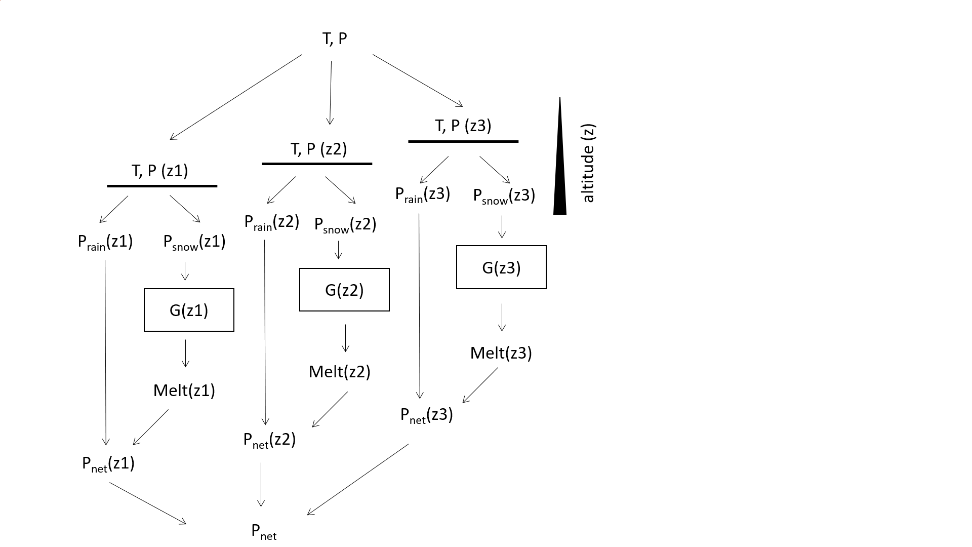
temperature and precipitation as inputs, it calculates snow accumulation and melting.
It is implemented according to the R airGR package (Coron et al., 2017).
The following list summarises the main components of snow_cn:
Altitude adjustment of precipitation and temperature data.
Division into liquid and solid precipitation.
Calculation of the thermal state of the snow layer.
Potential melt as a function of temperature and thermal state of the snow layer.
Estimation of snow-covered area.
Actual melt, dependent on potential melt and snow-covered area.
Net rainfall, calculated as the sum of liquid precipitation and actual melt.
The following figure shows the general structure of snow_cn based on a configuration
of three layers:
Integration tests
Note
When new to HydPy, consider reading section Integration Tests first.
Example 1
The first example uses the dataset L0123001 from the airGR package. It spans 61 days from April to the end of May, with a simulation step of 1 day snd including several precipitation events:
>>> from hydpy import pub
>>> pub.timegrids = "1990-04-01", "1990-06-01", "1d"
We create a model instance and connect it to an element:
>>> from hydpy.models.snow_cn import *
>>> parameterstep("1d")
>>> from hydpy import Element
>>> land = Element("land")
>>> land.model = model
We initialise a test function object that prepares and runs the tests, and prints and plots their results:
>>> from hydpy import IntegrationTest
>>> IntegrationTest.plotting_options.axis1 = inputs.p, fluxes.pnet
>>> IntegrationTest.plotting_options.axis2 = inputs.t, states.g
>>> test = IntegrationTest(land)
>>> test.dateformat = "%d.%m."
In this first example, we turn off the model’s hysteresis functionality:
>>> hysteresis(False)
We prepare five snow layers and set their areas and altitudes with the helper method
prepare_layers():
>>> nlayers(5)
>>> hypsodata = [
...     286.0, 309.0, 320.0, 327.0, 333.0, 338.0, 342.0, 347.0, 351.0, 356.0, 360.0,
...     365.0, 369.0, 373.0, 378.0, 382.0, 387.0, 393.0, 399.0, 405.0, 411.0, 417.0,
...     423.0, 428.0, 434.0, 439.0, 443.0, 448.0, 453.0, 458.0, 463.0, 469.0, 474.0,
...     480.0, 485.0, 491.0, 496.0, 501.0, 507.0, 513.0, 519.0, 524.0, 530.0, 536.0,
...     542.0, 548.0, 554.0, 560.0, 566.0, 571.0, 577.0, 583.0, 590.0, 596.0, 603.0,
...     609.0, 615.0, 622.0, 629.0, 636.0, 642.0, 649.0, 656.0, 663.0, 669.0, 677.0,
...     684.0, 691.0, 698.0, 706.0, 714.0, 722.0, 730.0, 738.0, 746.0, 754.0, 762.0,
...     770.0, 777.0, 786.0, 797.0, 808.0, 819.0, 829.0, 841.0, 852.0, 863.0, 875.0,
...     887.0, 901.0, 916.0, 934.0, 952.0, 972.0, 994.0, 1012.0, 1029.0, 10540.0,
...     10800.0, 11250.0, 12780.0
... ]
>>> model.prepare_layers(hypsodata=hypsodata)
The following values for the CemaNeige parameters CN1 and CN2 stem from the
mentioned dataset:
>>> cn1(0.962)
>>> cn2(2.249)
In contrast, CN4 is not configurable in the airGR implementation but is set to 0.9 as
a constant:
>>> cn4(0.9)
Mean annual solid precipitation is 83 mm:
>>> meanansolidprecip(83.0)
snow_cn performs elevation adjustments for precipitation via parameter GradP and
for air temperature via parameter GradTMean. GradP requires only a single value:
>>> gradp(0.00041)
However, GradTMean allows individual values to be defined for each day of the year.
We select the values for France proposed by Valéry (2010) relevant for the
considered simulation period:
>>> gradtmean(nan)
>>> gradtmean.values[90:152] = [
...     0.59, 0.591, 0.591, 0.592, 0.593, 0.593, 0.594, 0.595, 0.595, 0.596, 0.596,
...     0.597, 0.597, 0.597, 0.598, 0.598, 0.598, 0.599, 0.599, 0.599, 0.599, 0.6, 0.6,
...     0.6, 0.6, 0.6, 0.601, 0.601, 0.601, 0.601, 0.601, 0.601, 0.601, 0.601, 0.601,
...     0.601, 0.601, 0.601, 0.601, 0.601, 0.602, 0.602, 0.602, 0.602, 0.602, 0.602,
...     0.602, 0.602, 0.602, 0.602, 0.602, 0.602, 0.602, 0.602, 0.602, 0.602, 0.602,
...     0.602, 0.602, 0.602, 0.602, 0.602]
In the airGR package, the measurement height of air temperature and precipitation can
be set independently of the catchment height. Since it is now common to interpolate
station data during pre-processing, we decided to remove this parameter and instead
introduce the derived parameter ZMean, which is calculated from the layer heights.
To be consistent with the airGR test case, we set ZMean to 577, the original station
height:
>>> parameters.update()
>>> derived.zmean(577)
All initial conditions are zero:
>>> test.inits = (
...     (states.g, [0.0, 0.0, 0.0, 0.0, 0.0]),
...     (states.etg, [0.0, 0.0, 0.0, 0.0, 0.0]),
...     (states.gratio, [0.0, 0.0, 0.0, 0.0, 0.0]),
... )
The time series for precipitation and air temperature are taken from the sample data set:
>>> inputs.p.series = (
...     0.4, 0.0, 1.0, 1.6, 3.1, 0.0, 0.0, 0.0, 0.0, 2.4, 2.1, 0.8, 8.4, 16.1, 2.9,
...     0.0, 0.4, 12.2, 8.8, 6.3, 2.5, 0.0, 0.0, 1.7, 2.5, 9.9, 7.5, 0.3, 6.3, 4.6,
...     1.1, 0.0, 0.0, 0.0, 0.4, 9.1, 0.0, 13.4, 4.0, 0.0, 0.0, 8.6, 5.3, 2.5, 1.8,
...     0.0, 2.4, 13.3, 5.8, 4.3, 20.0, 9.8, 2.1, 1.6, 3.7, 0.2, 0.0, 0.0, 0.1, 0.7,
...     2.2)
>>> inputs.t.series = (
...     7.2, 7.1, 6.4, 7.4, 7.5, 4.3, 3.5, 3.5, 4.5, 5.0, 1.9, 1.8, 3.0, 1.3, 0.2, 1.8,
...     1.5, 3.7, 7.4, 7.6, 5.8, 6.0, 8.1, 8.1, 8.6, 8.7, 6.6, 8.8, 9.6, 9.2, 7.8, 8.0,
...     10.6, 13.8, 12.1, 7.7, 7.0, 10.0, 9.1, 11.3, 6.6, 7.4, 5.9, 7.6, 9.2, 11.8,
...     13.8, 12.1, 10.8, 11.7, 11.1, 7.3, 8.0, 10.3, 8.0, 10.4, 14.0, 14.2, 14.9,
...     15.6, 16.3)
During the highest precipitation event in mid-April, air temperatures are close to 0°C. Hence, especially in the highest of the fifth layers, a significant snowpack builds up, which then melts down mostly in the rest of April. In May, none of the additional precipitation falls as snow, but instead of vanishing completely, the snow pack continues to decline exponentially:
>>> test("snow_cn_example1", update_parameters=False)
Click to see the table
Click to see the graphExample 2
In the second example, we activate the model’s hysteresis feature and adjust the test setting so that it can actually come into play:
>>> pub.timegrids = "1990-01-01", "1990-01-16", "1d"
>>> hysteresis(True)
>>> cn3(20.0)
>>> cn4(0.4)
>>> gradtmean.values[:16] = [
...     0.434, 0.434, 0.435, 0.436, 0.437, 0.439, 0.44, 0.441, 0.442, 0.444, 0.445,
...     0.446, 0.448, 0.45, 0.451, 0.453]
>>> parameters.update()
>>> derived.zmean(577)
>>> test.inits = (
...     (states.g, [10.0, 15.0, 20.0, 30.0, 40.0]),
...     (states.etg, [0.0, 0.0, 0.0, 0.0, 0.0]),
...     (states.gratio, [0.8, 0.8, 0.8, 0.8, 0.8]),
...     (logs.glocalmax, derived.gthresh),
... )
>>> inputs.t.series = (
...     5.0, 5.0, 5.0, 5.0, 5.0, 5.0, -1.0, -1.0, 5.0, 5.0, 5.0, 5.0, 5.0, 5.0, 5.0
... )
>>> inputs.p.series = (
...     0.0, 0.0, 0.0, 0.0, 0.0, 0.0, 10.0, 10.0, 0.0, 0.0, 0.0, 0.0, 0.0, 0.0, 0.0
... )
The hysterisis effect increases snow melt, resulting in a peak net precipitation of 7.1 mm/d (instead of 6.0 mm/d with hysteresis turned off):
>>> test("snow_cn_hyst_example2", update_parameters=False)
Click to see the table
Click to see the graph- class hydpy.models.snow_cn.Model[source]
Bases:
BaseModelHydPy-Snow-CemaNeige-T-Mean (CemaNeige model with mean air temperature as input).
- The following “run methods” are called in the given sequence during each simulation step:
Calc_PLayer_V1Adjust the precipitation to the altitude for the snow layers according to Valéry (2010).Calc_TLayer_V1Calculate the mean temperature for each snow layer based on methodReturn_T_V1.Calc_SolidFractionPrecipitation_V1Calculate the solid precipitation fraction for each snow layer according to USACE (1956).Calc_PRainLayer_V1Calculate the liquid part of precipitation (USACE, 1956).Calc_PSnowLayer_V1Calculate the frozen part of precipitation.Update_G_V1Add the snowfall to each layer’s snow pack.Calc_ETG_V1Update the thermal state of each snow layer.Calc_PotMelt_V1Calculate the potential melt for each snow layer.Update_GRatio_GLocalMax_V1Calculate the fraction of the snow-covered area for each snow layer and updateGLocalMaxbefore calculating the snowmelt.Calc_Melt_V1Calculate the actual snow melt for each layer.Update_G_V2Remove the snowmelt from the snowpack.Update_GRatio_GLocalMax_V2Calculate the fraction of the snow-covered area for each snow layer and updateGLocalMaxafter calculating the snowmelt.Calc_PNetLayer_V1Sum the rainfall and the actual snow melt for each layer.Calc_PNet_V1Calculate the catchment’s average net rainfall.
- The following “additional methods” might be called by one or more of the other methods or are meant to be directly called by the user:
Return_T_V1Return the altitude-adjusted temperature.
- DOCNAME = ('Snow-CemaNeige-T-Mean', 'CemaNeige model with mean air temperature as input')
- REUSABLE_METHODS = ()
- class hydpy.models.snow_cn.ControlParameters(master: Parameters[TM_co], cls_fastaccess: type[FastAccessParameter] | None = None, cymodel: CyModelProtocol | None = None)
Bases:
ControlParametersControl parameters of model snow_cn.
- The following classes are selected:
NLayers()Number of snow layers [-].ZLayers()Height of each snow layer [m].LayerArea()Area of snow layer as a percentage of total area [-].GradP()Altitude gradient of precipitation [1/m].GradTMean()Altitude gradient of daily mean air temperature for each day of the year [°C/100m].MeanAnSolidPrecip()Mean annual solid precipitation [mm/a].CN1()Temporal weighting coefficient for the snow pack’s thermal state [-].CN2()Degree-day melt coefficient [mm/°C/T].CN3()Accumulation threshold [mm].CN4()Fraction of annual snowfall defining the melt threshold [-].Hysteresis()Flag that indicates whether hysteresis of build-up and melting of the snow cover should be considered [-].
- class hydpy.models.snow_cn.DerivedParameters(master: Parameters[TM_co], cls_fastaccess: type[FastAccessParameter] | None = None, cymodel: CyModelProtocol | None = None)
Bases:
DerivedParametersDerived parameters of model snow_cn.
- class hydpy.models.snow_cn.FactorSequences(master: Sequences[TM_co], cls_fastaccess: type[TypeFastAccess_co] | None = None, cymodel: CyModelProtocol | None = None)
Bases:
FactorSequencesFactor sequences of model snow_cn.
- The following classes are selected:
TLayer()Mean air temperature of each snow layer [°C].SolidFractionPrecipitation()Solid fraction of precipitation of each snow layer [-].
- class hydpy.models.snow_cn.FixedParameters(master: Parameters[TM_co], cls_fastaccess: type[FastAccessParameter] | None = None, cymodel: CyModelProtocol | None = None)
Bases:
FixedParametersFixed parameters of model snow_cn.
- The following classes are selected:
ZThreshold()Altitude threshold for constant precipitation [m].MinMelt()Minimum ratio of actual to potential melt [-].TThreshSnow()Temperature below which all precipitation falls as snow [°C].TThreshRain()Temperature above which all precipitation falls as rain [°C].MinG()Amount of snow below which actual melt can be equal to potential melt [mm].
- class hydpy.models.snow_cn.FluxSequences(master: Sequences[TM_co], cls_fastaccess: type[TypeFastAccess_co] | None = None, cymodel: CyModelProtocol | None = None)
Bases:
FluxSequencesFlux sequences of model snow_cn.
- The following classes are selected:
PLayer()Precipitation of each snow layer [mm/T].PSnowLayer()Snowfall of each snow layer [mm/T].PRainLayer()Rainfall of each snow layer [mm/T].PotMelt()Potential snow melt of each snow layer [mm/T].Melt()Actual snow melt of each snow layer [mm/T].PNetLayer()Net precipitation of each snow layer [mm/T].PNet()Net precipitation of the complete catchment [mm/T].
- class hydpy.models.snow_cn.InputSequences(master: Sequences[TM_co], cls_fastaccess: type[TypeFastAccess_co] | None = None, cymodel: CyModelProtocol | None = None)
Bases:
InputSequencesInput sequences of model snow_cn.
- class hydpy.models.snow_cn.LogSequences(master: Sequences[TM_co], cls_fastaccess: type[TypeFastAccess_co] | None = None, cymodel: CyModelProtocol | None = None)
Bases:
LogSequencesLog sequences of model snow_cn.
- The following classes are selected:
GLocalMax()Local melt threshold [mm].
- class hydpy.models.snow_cn.StateSequences(master: Sequences[TM_co], cls_fastaccess: type[TypeFastAccess_co] | None = None, cymodel: CyModelProtocol | None = None)
Bases:
StateSequencesState sequences of model snow_cn.