armatools

This module provides additional features for module iuhtools, related to Autoregressive-Moving Average (ARMA) models.

Module armatools implements the following members:

• MA Moving Average Model.

• ARMA Autoregressive-Moving Average model.

---

class hydpy.auxs.armatools.MA(iuh=None, coefs=None)

Bases: object

Moving Average Model.

The MA coefficients can be set manually:

>>> from hydpy import MA
>>> ma = MA(coefs=(0.8, 0.2))
>>> ma
MA(coefs=(0.8, 0.2))
>>> ma.coefs = 0.2, 0.8
>>> ma
MA(coefs=(0.2, 0.8))

Otherwise they are determined by method update_coefs(). But this requires that an integrable function object is given. Usually, this function object is an IUH subclass object, but (as in the following example) other function objects defining instantaneuous unit hydrographs are accepted. However, they should be well-behaved (e.g. be relatively smooth, unimodal, strictly positive, unity integral surface in the positive range).

For educational purposes, some discontinuous functions are applied in the following. One can suppress the associated warning messages with the following commands:

>>> import warnings
>>> from scipy import integrate
>>> warnings.filterwarnings("ignore", category=integrate.IntegrationWarning)

The first example is a simple rectangle impuls:

>>> ma = MA(iuh=lambda x: 0.05 if x < 20.0 else 0.0)
>>> ma.iuh.moment1 = 10.0
>>> ma
MA(coefs=(0.025, 0.05, 0.05, 0.05, 0.05, 0.05, 0.05, 0.05, 0.05, 0.05,
          0.05, 0.05, 0.05, 0.05, 0.05, 0.05, 0.05, 0.05, 0.05, 0.05,
          0.025))

The number of the coefficients can be modified by changing the class attribute smallest_coeff:

>>> ma.smallest_coeff = 0.03
>>> ma.update_coefs()
>>> ma
MA(coefs=(0.025641, 0.051282, 0.051282, 0.051282, 0.051282, 0.051282,
          0.051282, 0.051282, 0.051282, 0.051282, 0.051282, 0.051282,
          0.051282, 0.051282, 0.051282, 0.051282, 0.051282, 0.051282,
          0.051282, 0.051282))

The first two central moments of the time delay are a usefull measure for describing the operation of a MA model:

>>> ma = MA(iuh=lambda x: 1.0 if x < 1.0 else 0.0)
>>> ma.iuh.moment1 = 0.5
>>> ma
MA(coefs=(0.5, 0.5))
>>> from hydpy import round_
>>> round_(ma.moments, 6)
0.5, 0.5

The first central moment is the weigthed time delay (mean lag time). The second central moment is the weighted mean deviation from the mean lag time (diffusion).

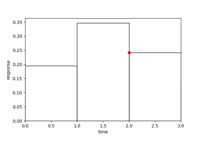
MA objects can return the turning point in the recession part of their MA coefficients. This can be demonstrated for the right side of the probability density function of the normal distribution with zero mean and a standard deviation (turning point) of 10:

>>> from scipy import stats
>>> ma = MA(iuh=lambda x: 2.0*stats.norm.pdf(x, 0.0, 2.0))
>>> ma.iuh.moment1 = 1.35
>>> ma
MA(coefs=(0.195417, 0.346659, 0.24189, 0.13277, 0.057318, 0.019458,
          0.005193, 0.001089, 0.00018, 0.000023, 0.000002, 0.0, 0.0))
>>> round_(ma.turningpoint)
2, 0.24189

Note that the first returned value is the index of the the MA coefficient closest to the turning point, and not a high precision estimate of the real turning point of the instantaneous unit hydrograph.

You can also use the following ploting command to verify the position of the turning point, which is printed as a red dot.

>>> ma.plot(threshold=0.9)

The turning point detection also works for functions which include both a rising and a falling limb. This can be shown shifting the normal distribution to the right:

>>> ma.iuh = lambda x: 1.02328*stats.norm.pdf(x, 4.0, 2.0)
>>> ma.iuh.moment1 = 3.94
>>> ma.update_coefs()
>>> ma
MA(coefs=(0.019322, 0.067931, 0.12376, 0.177364, 0.199966, 0.177364,
          0.12376, 0.067931, 0.029326, 0.009956, 0.002657, 0.000557,
          0.000092, 0.000012, 0.000001, 0.0, 0.0))
>>> round_(ma.turningpoint)
6, 0.12376

When no turning point can be detected, an error is raised:

>>> ma.coefs = 1.0, 1.0, 1.0
>>> ma.turningpoint
Traceback (most recent call last):
...
RuntimeError: Not able to detect a turning point in the impulse response defined by the MA coefficients `1.0, 1.0, 1.0`.

The next example requires reactivating the warning suppressed above:

>>> warnings.filterwarnings("error", category=integrate.IntegrationWarning)

The MA coefficients need to be approximated numerically. For very spiky response function, the underlying integration algorithm might fail. Then it is assumed that the complete mass of the response function is placed at a single delay time, defined by the property moment1 of the instantaneous unit hydrograph. Hopefully, this leads to plausible results. However, we raise an additional warning message to allow users to determine the coefficients by a different approach:

>>> ma.iuh = lambda x: 10.0 if 4.2 < x <= 4.3 else 0.0
>>> ma.iuh.moment1 = 4.25
>>> ma.update_coefs()   
Traceback (most recent call last):
...
UserWarning: During the determination of the MA coefficients corresponding to the instantaneous unit hydrograph ... a numerical integration problem occurred.  Please check the calculated coefficients: 0.0, 0.0, 0.0, 0.0, 0.75, 0.25.
>>> ma
MA(coefs=(0.0, 0.0, 0.0, 0.0, 0.75, 0.25))

For very steep response functions, numerical integration might fail:

>>> ma = MA(iuh=lambda x: stats.norm.pdf(x, 4.0, 1e-6))
>>> ma.iuh.moment1 = 4.0
>>> ma.update_coefs()   
Traceback (most recent call last):
...
RuntimeError: Cannot determine the MA coefficients corresponding to the instantaneous unit hydrograph `...`.

For very fast responses, there should be only one MA coefficient that has the value 1. Method update_coefs() provides a heuristic for such cases where numerical integration fails. As we are not sure that this heuristic works in all possible cases, update_coefs() raises the following warning in such cases:

>>> ma = MA(iuh=lambda x: 1e6*numpy.exp(-1e6*x))
>>> ma.iuh.moment1 = 6.931e-7
>>> ma 
Traceback (most recent call last):
...
UserWarning: During the determination of the MA coefficients corresponding to the instantaneous unit hydrograph `...` a numerical integration problem occurred.  Please check the calculated coefficients: 1.0.

>>> ma
MA(coefs=(1.0,))

smallest_coeff: float = 1e-09

Smalles MA coefficient to be determined at the end of the response.

coefs

ndarray containing all MA coefficents.

property order: int

MA order.

update_coefs() → None

(Re)calculate the MA coefficients based on the instantaneous unit hydrograph.

property turningpoint: tuple[int, float]

Turning point (index and value tuple) in the recession part of the MA approximation of the instantaneous unit hydrograph.

property delays: ndarray[Any, dtype[float64]]

Time delays related to the individual MA coefficients.

property moments: tuple[float, float]

The first two time delay weighted statistical moments of the MA coefficients.

plot(threshold=None, **kwargs) → None

Barplot of the MA coefficients.

class hydpy.auxs.armatools.ARMA(ma_model=None, ar_coefs=None, ma_coefs=None)

Bases: object

Autoregressive-Moving Average model.

One can set all ARMA coefficients manually:

>>> from hydpy import MA, ARMA, print_matrix
>>> arma = ARMA(ar_coefs=(0.5,), ma_coefs=(0.3, 0.2))
>>> print_matrix(arma.coefs)
| 0.5 |
| 0.3, 0.2 |
>>> arma
ARMA(ar_coefs=(0.5,),
     ma_coefs=(0.3, 0.2))

>>> arma.ar_coefs = ()
>>> arma.ma_coefs = range(20)
>>> arma
ARMA(ar_coefs=(),
     ma_coefs=(0.0, 1.0, 2.0, 3.0, 4.0, 5.0, 6.0, 7.0, 8.0, 9.0, 10.0,
               11.0, 12.0, 13.0, 14.0, 15.0, 16.0, 17.0, 18.0, 19.0))

Alternatively, they are determined by method update_coefs(), which requires an available MA. We use the MA model based on the shifted normal distribution of the documentation on class MA as an example:

>>> from scipy import stats
>>> ma = MA(iuh=lambda x: 1.02328 * stats.norm.pdf(x, 4.0, 2.0))
>>> ma.iuh.moment1 = 3.94
>>> arma = ARMA(ma_model=ma)
>>> arma
ARMA(ar_coefs=(0.680483, -0.228511, 0.047283, -0.006022, 0.000377),
     ma_coefs=(0.019322, 0.054783, 0.08195, 0.107757, 0.104458,
               0.07637, 0.041095, 0.01581, 0.004132, 0.000663,
               0.00005))

To verify that the ARMA model approximates the MA model with sufficient accuracy, one can query the achieved relative rmse value (rel_rmse) or check the central moments of their responses to the standard delta time impulse:

>>> from hydpy import round_
>>> round_(arma.rel_rmse)
0.0
>>> round_(ma.moments)
4.110496, 1.926798
>>> round_(arma.moments)
4.110496, 1.926798

On can check the accuray of the approximation directly via the property dev_moments, which is the sum of the absolute values of the deviations of both methods:

>>> round_(arma.dev_moments)
0.0

For the first six digits, there is no difference. However, the total number of coefficients is only reduced by one:

>>> ma.order
17
>>> arma.order
(5, 11)

To reduce the determined number or AR coefficients, one can set a higher AR-related tolerance value:

>>> arma.max_rel_rmse = 1e-3
>>> arma.update_coefs()
>>> arma
ARMA(ar_coefs=(0.788899, -0.256436, 0.034256),
     ma_coefs=(0.019322, 0.052688, 0.075125, 0.096488, 0.089453,
               0.060854, 0.029041, 0.008929, 0.001397, 0.000001,
               -0.000004, 0.00001, -0.000008, -0.000009, -0.000004,
               -0.000001))

The number of AR coeffcients is actually reduced. However, there are now even more MA coefficients, possibly trying to compensate the lower accuracy of the AR coefficients, and there is a slight decrease in the precision of the moments:

>>> arma.order
(3, 16)
>>> round_(arma.moments)
4.110497, 1.926804
>>> round_(arma.dev_moments)
0.000007

To also reduce the number of MA coefficients, one can set a higher MA-related tolerance value:

>>> arma.max_dev_coefs = 1e-3
>>> arma.update_coefs()
>>> arma
ARMA(ar_coefs=(0.788888, -0.256432, 0.034255),
     ma_coefs=(0.019321, 0.052687, 0.075124, 0.096486, 0.089452,
               0.060853, 0.02904, 0.008929, 0.001397))

Now the total number of coefficients is in fact decreased, and the loss in accuracy is still small:

>>> arma.order
(3, 9)
>>> round_(arma.moments)
4.110794, 1.927625
>>> round_(arma.dev_moments)
0.001125

Further relaxing the tolerance values results in even less coefficients, but also in some slightly negative responses to a standard impulse:

>>> arma.max_rel_rmse = 1e-2
>>> arma.max_dev_coefs = 1e-2
>>> from hydpy.core.testtools import warn_later
>>> with warn_later():
...     arma.update_coefs()
UserWarning: Note that the smallest response to a standard impulse of the determined ARMA model is negative (`-0.000336`).
>>> arma
ARMA(ar_coefs=(0.736954, -0.166457),
     ma_coefs=(0.01946, 0.05418, 0.077804, 0.098741, 0.091295,
               0.060797, 0.027226))
>>> arma.order
(2, 7)
>>> from hydpy import print_vector
>>> print_vector(arma.response)
0.01946, 0.068521, 0.125062, 0.1795, 0.202761, 0.180343, 0.12638,
0.063117, 0.025477, 0.008269, 0.001853, -0.000011, -0.000316,
-0.000231, -0.000118, -0.000048, -0.000016

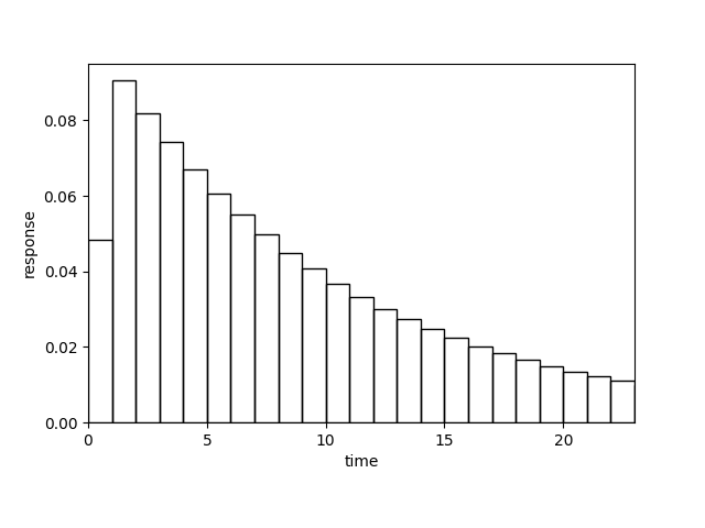
It seems to be hard to find a parameter efficient approximation to the MA model in the given example. Generally, approximating ARMA models to MA models is more beneficial when functions with long tails are involved. The most extreme example would be a simple exponential decline:

>>> import numpy
>>> ma = MA(iuh=lambda x: 0.1*numpy.exp(-0.1*x))
>>> ma.iuh.moment1 = 6.932
>>> arma = ARMA(ma_model=ma)

In the given example a number of 185 MA coefficients can be reduced to a total number of three ARMA coefficients with no relevant loss of accuracy:

>>> ma.order
185
>>> arma.order
(1, 2)
>>> round_(arma.dev_moments)
0.0

Use the following plotting command to see why 2 MA coeffcients instead of one are required in the above example:

>>> arma.plot(threshold=0.9)

Violations of the tolerance values are reported as warnings:

>>> arma.max_dev_coefs = 0.0
>>> arma.update_coefs()
Traceback (most recent call last):
...
UserWarning: Method `update_ma_coefs` is not able to determine the MA coefficients of the ARMA model with the desired accuracy.  You can set the tolerance value ´max_dev_coefs` to a higher value.  An accuracy of `0.000000000925` has been reached using `185` MA coefficients.
>>> arma.max_rel_rmse = 0.0
>>> arma.update_coefs()
Traceback (most recent call last):
...
UserWarning: Method `update_ar_coefs` is not able to determine the AR coefficients of the ARMA model with the desired accuracy.  You can either set the tolerance value `max_rel_rmse` to a higher value or increase the allowed `max_ar_order`.  An accuracy of `0.0` has been reached using `10` coefficients.
>>> arma.ma.coefs = 1.0, 1.0, 1.0
>>> arma.update_coefs()
Traceback (most recent call last):
...
UserWarning: Not able to detect a turning point in the impulse response defined by the MA coefficients `1.0, 1.0, 1.0`.

When getting such warnings, you need to inspect the achieved coefficients manually. In the last case, when the turning point detection failed, method update_coefs() simplified the ARMA to the original MA model, which is safe but not always a good choice:

>>> import warnings
>>> with warnings.catch_warnings():
...     warnings.simplefilter("ignore")
...     arma.update_coefs()
>>> arma
ARMA(ar_coefs=(),
     ma_coefs=(0.333333, 0.333333, 0.333333))

max_ar_order: int = 10

Maximum number of AR coefficients that are to be determined by method update_coefs().

max_rel_rmse: float = 1e-06

Maximum relative root mean squared error to be accepted by method update_coefs().

max_dev_coefs: float = 1e-06

Maximum deviation of the sum of all coefficents from one to be accepted by method update_coefs().

property rel_rmse: float

Relative root mean squared error the last time achieved by method update_coefs().

>>> from hydpy.auxs.armatools import ARMA
>>> ARMA().rel_rmse
Traceback (most recent call last):
...
RuntimeError: The relative root mean squared error has not been determined so far.

ar_coefs

The AR coefficients of the ARMA model.

property ar_coefs does not recalculate already defined coefficients automatically for efficiency:

>>> from hydpy import MA, ARMA, print_vector
>>> arma = ARMA(ar_coefs=(0.5,), ma_coefs=(0.3, 0.2))
>>> from scipy import stats
>>> arma.ma = MA(iuh=lambda x: 1.02328 * stats.norm.pdf(x, 4.0, 2.0))
>>> arma.ma.iuh.moment1 = 3.94
>>> print_vector(arma.ar_coefs)
0.5

You can trigger the recalculation by removing the available coefficients first:

>>> del arma.ar_coefs
>>> print_vector(arma.ar_coefs)
0.680483, -0.228511, 0.047283, -0.006022, 0.000377
>>> arma
ARMA(ar_coefs=(0.680483, -0.228511, 0.047283, -0.006022, 0.000377),
     ma_coefs=(0.019322, 0.054783, 0.08195, 0.107757, 0.104458,
               0.07637, 0.041095, 0.01581, 0.004132, 0.000663,
               0.00005))

ma_coefs

The MA coefficients of the ARMA model.

property ma_coefs does not recalculate already defined coefficients automatically for efficiency:

>>> from hydpy import MA, ARMA, print_vector
>>> arma = ARMA(ar_coefs=(0.5,), ma_coefs=(0.3, 0.2))
>>> from scipy import stats
>>> arma.ma = MA(iuh=lambda x: 1.02328 * stats.norm.pdf(x, 4.0, 2.0))
>>> arma.ma.iuh.moment1 = 3.94
>>> print_vector(arma.ma_coefs)
0.3, 0.2

You can trigger the recalculation by removing the available coefficients first:

>>> del arma.ma_coefs
>>> print_vector(arma.ma_coefs)
0.019322, 0.054783, 0.08195, 0.107757, 0.104458, 0.07637, 0.041095,
0.01581, 0.004132, 0.000663, 0.00005
>>> arma
ARMA(ar_coefs=(0.680483, -0.228511, 0.047283, -0.006022, 0.000377),
     ma_coefs=(0.019322, 0.054783, 0.08195, 0.107757, 0.104458,
               0.07637, 0.041095, 0.01581, 0.004132, 0.000663,
               0.00005))

property coefs: tuple[ndarray[Any, dtype[float64]], ndarray[Any, dtype[float64]]]

Tuple containing both the AR and the MA coefficients.

property ar_order: int

Number of AR coefficients.

property ma_order: int

Number of MA coefficients

property order: tuple[int, int]

Number of both the AR and the MA coefficients.

update_coefs() → None

Determine both the AR and the MA coefficients.

property effective_max_ar_order: int

The maximum number of AR coefficients that shall or can be determined.

It is the minimum of max_ar_order and the number of coefficients of the pure MA after their turning point.

update_ar_coefs() → None

Determine the AR coefficients.

The number of AR coefficients is subsequently increased until the required precision max_rel_rmse or the maximum number of AR coefficients (see effective_max_ar_order) is reached. In the second case, update_ar_coefs() raises a warning.

property dev_moments: float

Sum of the absolute deviations between the central moments of the instantaneous unit hydrograph and the ARMA approximation.

norm_coefs() → None

Multiply all coefficients by the same factor, so that their sum becomes one.

property sum_coefs: float

The sum of all AR and MA coefficients

property dev_coefs: float

Absolute deviation of sum_coefs from one.

calc_all_ar_coefs(ar_order: int, ma_model: MA) → None

Determine the AR coeffcients based on a least squares approach.

The argument ar_order defines the number of AR coefficients to be determined. The argument ma_order defines a pure MA model. The least squares approach is applied on all those coefficents of the pure MA model, which are associated with the part of the recession curve behind its turning point.

The attribute rel_rmse is updated with the resulting relative root mean square error.

static get_a(values, n)

Extract the independent variables of the given values and return them as a matrix with n columns in a form suitable for the least squares approach applied in method update_ar_coefs().

static get_b(values, n)

Extract the dependent variables of the values in a vector with n entries in a form suitable for the least squares approach applied in method update_ar_coefs().

update_ma_coefs() → None

Determine the MA coefficients.

The number of MA coefficients is subsequently increased until the required precision (max_dev_coefs) or the or the order of the original MA model is reached. In the second case, update_ma_coefs() raises a warning.

calc_next_ma_coef(ma_order, ma_model) → None

Determine the MA coefficients of the ARMA model based on its predetermined AR coefficients and the MA ordinates of the given MA model.

The MA coefficients are determined one at a time, beginning with the first one. Each ARMA MA coefficient in set in a manner that allows for the exact reproduction of the equivalent pure MA coefficient with all relevant ARMA coefficients.

property response: ndarray[Any, dtype[float64]]

Return the response to a standard dt impulse.

property moments: tuple[float, float]

The first two time delay weighted statistical moments of the ARMA response.

plot(threshold=None, **kwargs) → None

Barplot of the ARMA response.