ppolytools

This module implements interpolation approaches based on piecewise polynomials required for some models implemented in the HydPy framework.

The relevant models perform the interpolation during simulation runs, which is why we implement the related methods in the Cython extension module ppolyutils.

Module ppolytools implements the following members:

• Poly Parameter handler for a power series representation of a single polynomial function.

• PPoly Piecewise polynomial interpolator.

---

class hydpy.auxs.ppolytools.Poly(x0: float, cs: tuple[float, ...])

Bases: NamedTuple

Parameter handler for a power series representation of a single polynomial function.

The following Poly object corresponds to the polynomial function \(f(x) = 2 + 3 \cdot (x - 1) + 4 \cdot (x - 1)^2\):

>>> from hydpy import Poly
>>> p = Poly(x0=1.0, cs=(2.0, 3.0, 4.0))

Proper application of the constant and all coefficients for \(x = 3\) results in 24:

>>> x = 3.0
>>> p.cs[0] + p.cs[1] * (x - p.x0) + p.cs[2] * (x - p.x0) ** 2
24.0

x0: float

Constant of the power series.

cs: tuple[float, ...]

Coefficients of the power series.

assignrepr(prefix: str) → str

Return a string representation of the actual Poly object prefixed with the given string.

>>> from hydpy import Poly
>>> poly = Poly(x0=1.0/3.0, cs=(2.0, 3.0, 4.0/3.0))
>>> poly
Poly(x0=0.333333, cs=(2.0, 3.0, 1.333333))
>>> print(poly.assignrepr(prefix="poly = "))
poly = Poly(x0=0.333333, cs=(2.0, 3.0, 1.333333))

class hydpy.auxs.ppolytools.PPoly(*polynomials: Poly)

Bases: InterpAlgorithm

Piecewise polynomial interpolator.

Class PPoly supports univariate data interpolation via multiple polynomial functions. Typical use cases are linear or spline interpolation. The primary purpose of PPoly is to allow for such interpolation within model equations (for example, to represent the relationship between water volume and water stage as in the model dam_v001). Then, the user selects PPoly as the interpolation algorithm employed by parameters derived from SimpleInterpolator (e.g. WaterVolume2WaterLevel) or SeasonalInterpolator (e.g. WaterLevel2FloodDischarge). However, one can apply PPoly also directly, as shown in the following examples.

You can prepare a PPoly object by handing multiple Poly objects to its constructor:

>>> from hydpy import Poly, PPoly
>>> ppoly = PPoly(Poly(x0=1.0, cs=(1.0,)),
...         Poly(x0=2.0, cs=(1.0, 1.0)),
...         Poly(x0=3.0, cs=(2.0, 3.0)))

Note that each power series constant (x0) also serves as a breakpoint. Each x0 value defines the lower bound of the interval for which the polynomial is valid. The only exception affects the first Poly object. Here, x0 also serves as the power series constant but not as a breakpoint. Hence, PPoly uses the first polynomial for extrapolation into the negative range (as it uses the last polynomial for extrapolating into the positive range). The following equation, which reflects the configuration of the prepared interpolator, should clarify this definition:

\[\begin{split}f(x) = \begin{cases} 1 &|\ x < 2 \\ 1 + x - 2 &|\ 2 \leq x < 3 \\ 2 + 3 \cdot (x - 3) &|\ 3 \leq x \end{cases}\end{split}\]

For applying ppoly, we need to set the input value before calling calculate_values():

>>> ppoly.inputs[0] = 2.5
>>> ppoly.calculate_values()
>>> from hydpy import round_
>>> round_(ppoly.outputs[0])
1.5

The same holds when calling method calculate_derivatives() for calculating first order derivatives:

>>> ppoly.calculate_derivatives(0)
>>> round_(ppoly.output_derivatives[0])
1.0

Use method print_table() or method plot() to inspect the results of ppoly within the relevant data range:

>>> ppoly.print_table([0.5, 1.0, 1.5, 2.0, 2.5, 3.0, 3.5])
x    y    dy/dx
0.5  1.0  0.0
1.0  1.0  0.0
1.5  1.0  0.0
2.0  1.0  1.0
2.5  1.5  1.0
3.0  2.0  3.0
3.5  3.5  3.0

>>> figure = ppoly.plot(xmin=0.0, xmax=4.0)
>>> from hydpy.core.testtools import save_autofig
>>> save_autofig("PPoly_base_example.png", figure=figure)

PPoly collects all constants and coefficients and provides access to them via properties x0s and cs available:

>>> from hydpy import print_matrix, print_vector
>>> print_vector(ppoly.x0s)
1.0, 2.0, 3.0
>>> print_matrix(ppoly.cs)
| 1.0, 0.0 |
| 1.0, 1.0 |
| 2.0, 3.0 |

Property nmb_ps reflects the total number of polynomials:

>>> ppoly.nmb_ps
3

Property nmb_cs informs about the number of relevant coefficients for each polynomial (the last non-negative coefficient is the last relevant one):

>>> print_vector(ppoly.nmb_cs)
1, 2, 2

You are free to manipulate both the breakpoints and the coefficients:

>>> ppoly.x0s = 1.0, 2.0, 2.5
>>> ppoly.cs[1, 1] = 2.0

>>> ppoly.polynomials
(Poly(x0=1.0, cs=(1.0,)), Poly(x0=2.0, cs=(1.0, 2.0)), Poly(x0=2.5, cs=(2.0, 3.0)))

>>> ppoly.print_table([0.5, 1.0, 1.5, 2.0, 2.5, 3.0, 3.5])
x    y    dy/dx
0.5  1.0  0.0
1.0  1.0  0.0
1.5  1.0  0.0
2.0  1.0  2.0
2.5  2.0  3.0
3.0  3.5  3.0
3.5  5.0  3.0

However, be aware that manipulating nmb_ps, nmb_cs, x0s, nmb_cs can cause severe problems, including program crashes. Hence, you should always call the verify() method after manipulating these properties, which checks the integrity of the current configuration of PPoly objects:

>>> ppoly.nmb_ps = 1
>>> ppoly.verify()
Traceback (most recent call last):
...
RuntimeError: While trying to verify parameter `ppoly` of element `?`, the following error occurred: The number of constants indicated by `nmb_ps` (1) does not agree with the actual number of constants held by vector `x0s` (3).

To change an existing PPoly object more safely, you can “call” it with different Poly objects, which overwrites all current information, as shown by the following example, defining only a single polynomial:

>>> ppoly(Poly(x0=-1.0, cs=(0.0, 0.0, 1.0)))
>>> ppoly.print_table([-3.0, -2.0, -1.0, 0.0, 1.0])
x     y    dy/dx
-3.0  4.0  -4.0
-2.0  1.0  -2.0
-1.0  0.0  0.0
0.0   1.0  2.0
1.0   4.0  4.0

Calling PPoly objects without any arguments results in the following error:

>>> ppoly()
Traceback (most recent call last):
...
ValueError: When calling an `PPoly` object, you need to define at least one polynomial function by passing at leas one `Poly` object.

classmethod from_data(xs: VectorFloat, ys: VectorFloat, method: Literal['linear'] | type[interpolate.CubicHermiteSpline] = 'linear') → PPoly

Prepare a PPoly object based on x-y data.

As explained in the main documentation on class PPoly, you are free to define an arbitrary number of polynomials, each with arbitrary constants and coefficients. However, one usually prefers functionally similar polynomials that standardised algorithms can compute. Method from_data() is a convenience function for following this route. So far, it supports linear interpolation and some spline techniques.

We start our explanations with a small and smooth x-y data set:

>>> xs = [1.0, 2.0, 3.0]
>>> ys = [1.0, 2.0, 3.5]

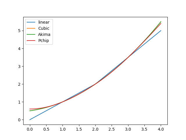
By default, method from_data() prepares everything for a piecewise linear interpolation:

>>> from hydpy import PPoly
>>> ppoly = PPoly.from_data(xs=xs, ys=ys)
>>> ppoly
PPoly(
    Poly(x0=1.0, cs=(1.0, 1.0)),
    Poly(x0=2.0, cs=(2.0, 1.5)),
)
>>> ppoly.print_table(xs=[1.9, 2.0, 2.1])
x    y     dy/dx
1.9  1.9   1.0
2.0  2.0   1.5
2.1  2.15  1.5
>>> figure = ppoly.plot(0.0, 4.0, label="linear")

Alternatively, PPoly can use the following scipy classes for determining higher-order polynomials:

>>> from scipy.interpolate import CubicSpline, Akima1DInterpolator, PchipInterpolator

For sufficiently smooth data, cubic spline interpolation is often a good choice, as it preserves much smoothness around breakpoints (helpful for reaching required accuracies when applying numerical integration algorithms):

>>> ppoly = PPoly.from_data(xs=xs, ys=ys, method=CubicSpline)
>>> ppoly
PPoly(
    Poly(x0=1.0, cs=(1.0, 0.75, 0.25)),
    Poly(x0=2.0, cs=(2.0, 1.25, 0.25)),
)
>>> ppoly.print_table(xs=[1.9, 2.0, 2.1])
x    y       dy/dx
1.9  1.8775  1.2
2.0  2.0     1.25
2.1  2.1275  1.3
>>> figure = ppoly.plot(0.0, 4.0, label="Cubic")

For the given data, the Akima spline results in the same coefficients as the cubic spline:

>>> ppoly = PPoly.from_data(xs=xs, ys=ys, method=Akima1DInterpolator)
>>> ppoly
PPoly(
    Poly(x0=1.0, cs=(1.0, 0.75, 0.25)),
    Poly(x0=2.0, cs=(2.0, 1.25, 0.25)),
)
>>> figure = ppoly.plot(0.0, 4.0, label="Akima")

The PCHIP (Piecewise Cubic Hermite Interpolating Polynomial) algorithm generally tends to less smooth interpolations:

>>> ppoly = PPoly.from_data(xs=xs, ys=ys, method=PchipInterpolator)
>>> ppoly
PPoly(
    Poly(x0=1.0, cs=(1.0, 0.75, 0.3, -0.05)),
    Poly(x0=2.0, cs=(2.0, 1.2, 0.35, -0.05)),
)
>>> ppoly.print_table(xs=[1.9, 2.0, 2.1])
x    y        dy/dx
1.9  1.88155  1.1685
2.0  2.0      1.2
2.1  2.12345  1.2685
>>> figure = ppoly.plot(0.0, 4.0, label="Pchip")

The following figure compares the linear and all spline interpolation results. As to be expected, the most sensible differences show in the interpolation ranges:

>>> _ = figure.gca().legend()
>>> from hydpy.core.testtools import save_autofig
>>> save_autofig("PPoly_data_smooth.png")

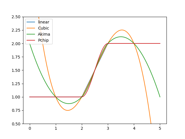
Next, we apply all four interpolation approaches on a non-smooth data set. Cubic interpolation is again the smoothest one but tends to overshoot, which can be problematic when violating physical constraints. Besides the linear approach, only the PCHIP interpolation always preserves monotonicity in the original data. The Akima interpolation appears as a good compromise between these two approaches:

>>> for method, label in (("linear", "linear"),
...                       (CubicSpline, "Cubic"),
...                       (Akima1DInterpolator, "Akima"),
...                       (PchipInterpolator, "Pchip")):
...     figure = PPoly.from_data(
...         xs=[1.0, 2.0, 3.0, 4.0], ys=[1.0, 1.0, 2.0, 2.0], method=method
...     ).plot(0.0, 5.0, label=label)
>>> _ = figure.gca().legend()
>>> _ = figure.gca().set_ylim((0.5, 2.5))
>>> save_autofig("PPoly_data_not_smooth.png")

Passing data sets with one or two x-y pairs works fine:

>>> PPoly.from_data(xs=[0.0], ys=[1.0])
PPoly(
    Poly(x0=0.0, cs=(1.0,)),
)

>>> PPoly.from_data(xs=[0.0, 1.0], ys=[2.0, 5.0])
PPoly(
    Poly(x0=0.0, cs=(2.0, 3.0)),
)

Empty data sets or data sets of different lengths result in the following error messages:

>>> PPoly.from_data(xs=[], ys=[])
Traceback (most recent call last):
...
ValueError: While trying to derive polynomials from the vectors `x` ([]) and `y` ([]), the following error occurred: Vectors `x` and `y` must not be empty.

>>> PPoly.from_data(xs=[0.0, 1.0], ys=[1.0, 2.0, 3.0])
Traceback (most recent call last):
...
ValueError: While trying to derive polynomials from the vectors `x` ([0.0 and 1.0]) and `y` ([1.0, 2.0, and 3.0]), the following error occurred: The lenghts of vectors `x` (2) and `y` (3) must be identical.

nmb_inputs: BaseProperty[Never, int]

The number of input values.

inputs: BaseProperty[Never, ndarray[Any, dtype[float64]]]

The current input values.

nmb_outputs: BaseProperty[Never, int]

The lastly calculated output values.

outputs: BaseProperty[Never, ndarray[Any, dtype[float64]]]

The lastly calculated output values.

output_derivatives: BaseProperty[Never, ndarray[Any, dtype[float64]]]

The lastly calculated first-order derivatives.

nmb_ps

The number of polynomials.

nmb_ps is “protected” (implemented by ProtectedProperty) for the sake of preventing segmentation faults when trying to access the related data from the underlying Cython extension class before allocation:

>>> from hydpy import PPoly
>>> ppoly = PPoly()
>>> ppoly.nmb_ps = 1
>>> ppoly.nmb_ps
1
>>> del ppoly.nmb_ps
>>> ppoly.nmb_ps
Traceback (most recent call last):
...
hydpy.core.exceptiontools.AttributeNotReady: Attribute `nmb_ps` of object `ppoly` has not been prepared so far.

nmb_cs

The number of relevant coefficients for each polynomial.

nmb_cs is “protected” (implemented by ProtectedProperty) for the sake of preventing segmentation faults when trying to access the related data from the underlying Cython extension class before allocation:

>>> from hydpy import PPoly, print_vector
>>> ppoly = PPoly()
>>> ppoly.nmb_cs = 1, 2
>>> print_vector(ppoly.nmb_cs)
1, 2
>>> del ppoly.nmb_cs
>>> ppoly.nmb_cs
Traceback (most recent call last):
...
hydpy.core.exceptiontools.AttributeNotReady: Attribute `nmb_cs` of object `ppoly` has not been prepared so far.

x0s

The power series constants of all polynomials.

x0s is “protected” (implemented by ProtectedProperty) for the sake of preventing segmentation faults when trying to access the related data from the underlying Cython extension class before allocation:

>>> from hydpy import PPoly, print_vector
>>> ppoly = PPoly()
>>> ppoly.x0s = 1.0, 2.0
>>> print_vector(ppoly.x0s)
1.0, 2.0
>>> del ppoly.x0s
>>> ppoly.x0s
Traceback (most recent call last):
...
hydpy.core.exceptiontools.AttributeNotReady: Attribute `x0s` of object `ppoly` has not been prepared so far.

cs

The power series coefficients of all polynomials.

cs is “protected” (implemented by ProtectedProperty) for the sake of preventing segmentation faults when trying to access the related data from the underlying Cython extension class before allocation:

>>> from hydpy import PPoly, print_matrix
>>> ppoly = PPoly()
>>> ppoly.cs = [[1.0, 2.0], [3.0, 4.0]]
>>> print_matrix(ppoly.cs)
| 1.0, 2.0 |
| 3.0, 4.0 |
>>> del ppoly.cs
>>> ppoly.cs
Traceback (most recent call last):
...
hydpy.core.exceptiontools.AttributeNotReady: Attribute `cs` of object `ppoly` has not been prepared so far.

calculate_values() → None

Calculate the output value based on the input values defined previously.

For more information, see the documentation on class PPoly.

calculate_derivatives(idx: int = 0) → None

Calculate the derivative of the output value with respect to the input value.

For more information, see the documentation on class PPoly.

property polynomials: tuple[Poly, ...]

The configuration of the current PPoly object, represented by a tuple of Poly objects.

>>> from hydpy import Poly, PPoly
>>> ppoly = PPoly(Poly(x0=1.0, cs=(1.0,)), Poly(x0=2.0, cs=(1.0, 1.0)))
>>> ppoly.polynomials
(Poly(x0=1.0, cs=(1.0,)), Poly(x0=2.0, cs=(1.0, 1.0)))

sort() → None

Sort the currently handled polynomials.

The power series constants held by array x0s also serve as breakpoints, defining the lower bounds of the intervals for which the available polynomials are valid. The algorithm underlying PPoly expects them in sorted order.

In the following example, we hand over two wrongly-ordered Poly objects:

>>> from hydpy import Poly, PPoly, print_matrix, print_vector
>>> ppoly = PPoly(Poly(x0=2.0, cs=(1.0, 1.0)), Poly(x0=1.0, cs=(1.0,)))
>>> ppoly.polynomials
(Poly(x0=2.0, cs=(1.0, 1.0)), Poly(x0=1.0, cs=(1.0,)))
>>> print_vector(ppoly.x0s)
2.0, 1.0
>>> print_vector(ppoly.nmb_cs)
2, 1
>>> print_matrix(ppoly.cs)
| 1.0, 1.0 |
| 1.0, 0.0 |

Method sort() sorts x0s and the related arrays nmb_cs and cs:

>>> ppoly.sort()
>>> ppoly.polynomials
(Poly(x0=1.0, cs=(1.0,)), Poly(x0=2.0, cs=(1.0, 1.0)))
>>> print_vector(ppoly.x0s)
1.0, 2.0
>>> print_vector(ppoly.nmb_cs)
1, 2
>>> print_matrix(ppoly.cs)
| 1.0, 0.0 |
| 1.0, 1.0 |

verify() → None

Raise a RuntimeError if the current PPoly object shows inconsistencies.

Note that PPoly never calls verify() automatically. Hence, we strongly advise applying it manually before using a new PPoly configuration the first time.

So far, method verify() reports the following problems:

>>> from hydpy import PPoly
>>> ppoly = PPoly(Poly(x0=2.0, cs=(1.0, 1.0)), Poly(x0=1.0, cs=(1.0,)))
>>> ppoly.verify()
Traceback (most recent call last):
...
RuntimeError: While trying to verify parameter `ppoly` of element `?`, the following error occurred: The constants held in vector `x0s` are not strictly increasing, which is necessary as they also serve as breakpoints for selecting the relevant polynomials.

>>> ppoly.sort()
>>> ppoly.verify()

>>> ppoly.nmb_cs[1] = 3
>>> ppoly.verify()
Traceback (most recent call last):
...
RuntimeError: While trying to verify parameter `ppoly` of element `?`, the following error occurred: The highest number of coefficients indicated by `nmb_cs` (3) is larger than the possible number of coefficients storable in the coefficient matrix `cs` (2).

>>> ppoly.cs = ppoly.cs[:1, :]
>>> ppoly.verify()
Traceback (most recent call last):
...
RuntimeError: While trying to verify parameter `ppoly` of element `?`, the following error occurred: The number of polynomials indicated by `nmb_ps` (2) does not agree with the actual number of coefficient arrays held by matrix `cs` (1).

>>> ppoly.x0s = ppoly.x0s[:1]
>>> ppoly.verify()
Traceback (most recent call last):
...
RuntimeError: While trying to verify parameter `ppoly` of element `?`, the following error occurred: The number of constants indicated by `nmb_ps` (2) does not agree with the actual number of constants held by vector `x0s` (1).

assignrepr(prefix: str, indent: int = 0) → str

Return a string representation of the actual PPoly object prefixed with the given string.

>>> from hydpy import Poly, PPoly
>>> ppoly = PPoly(Poly(x0=1.0, cs=(1.0,)), Poly(x0=2.0, cs=(1.0, 1.0)))
>>> ppoly
PPoly(
    Poly(x0=1.0, cs=(1.0,)),
    Poly(x0=2.0, cs=(1.0, 1.0)),
)
>>> print(ppoly.assignrepr(prefix="    ppoly = ", indent=4))
    ppoly = PPoly(
        Poly(x0=1.0, cs=(1.0,)),
        Poly(x0=2.0, cs=(1.0, 1.0)),
    )