lland_v1
Version 1 of the L-Land model is the simplest of our LARSIM-type models. In
contrast to lland_v3, it calculates snowmelt based on the straightforward degree-day
method. We created lland_v1 on behalf of the German Federal Institute of Hydrology
(BfG) for large-scale hydrological applications in central Europe.
The following list summarises the main components of lland_v1:
Simple routines for adjusting the meteorological input data
Configurable evapotranspiration methods by supporting the
AETModel_V1interfaceMixed precipitation within a definable temperature-range
An enhanced degree-day method for calculating snowmelt
A simple snow retention routine
Direct runoff generation based on the Xinanjiang model (Zhao, 1977)
Optional inclusion of a soil submodel following the
SoilModel_V1interfaceOne base flow, two interflow and two direct flow components
A freely configurable capillary rise routine
Options to limit the capacity of the base flow storage
Separate linear storages for modelling runoff concentration
Additional evaporation from water areas within the subcatchment
Optional evaporation from inflowing runoff
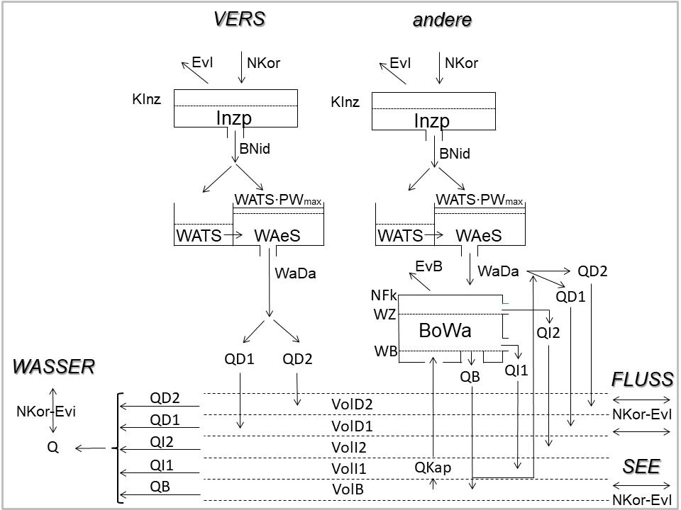
The following figure shows the general structure of L-Land Version 1. Besides water areas and sealed surfaces, all land-use types rely on the same process equations:
Integration tests
Note
When new to HydPy, consider reading section How to understand integration tests? first.
We perform all integration tests over five days, including an extreme precipitation event:
>>> from hydpy import pub
>>> pub.timegrids = "2000-01-01", "2000-01-05", "1h"
Next, we prepare a model instance:
>>> from hydpy.models.lland_v1 import *
>>> parameterstep("1h")
lland_v1 provides a type of optional routing approach, which adds the runoff from the
upstream sub-catchments to the runoff generated by the actual sub-catchment (see
example acre (routing)). This approach allows lland_v1 to subtract
water area evaporation not only from the runoff generated within the actual
sub-catchment but from the total runoff flowing through it (see example
water (routing)). The documentation on method Calc_QAH_V1 gives
further information.
The optionality of this routing approach results in different configuration
possibilities of the related Element objects. The element only requires an outlet
node if you do not want to use the routing approach (generally or because the relevant
catchment is a headwater catchment):
>>> from hydpy import Node, Element
>>> outlet = Node("outlet")
>>> land = Element("land", outlets=outlet)
>>> land.model = model
If you want to use the routing approach, you also need to define one or more inlet nodes, providing the inflowing runoff (we rely on such an element throughout the following examples but make our catchment effectively to a headwater by setting the inflow to zero most of the time):
>>> inlet = Node("inlet")
>>> land = Element("land", inlets=inlet, outlets=outlet)
>>> land.model = model
We focus on a single hydrological response unit with one square kilometre:
>>> nhru(1)
>>> ft(1.0)
>>> fhru(1.0)
acre (summer)
In the first example, arable land is the land-use class of our choice (for all other land-use types, except the ones mentioned below, the results were the same):
>>> lnk(ACKER)
The following set of control parameter values tries to configure application model
lland_v1 in a manner that allows retracing the influence of most of the different
implemented methods on the shown results:
>>> kg(1.2)
>>> kt(0.8)
>>> hinz(0.2)
>>> lai(4.0)
>>> treft(0.0)
>>> trefn(0.0)
>>> tgr(1.0)
>>> tsp(2.0)
>>> gtf(0.5)
>>> pwmax(1.4)
>>> wmax(200.0)
>>> fk(relative=0.5)
>>> pwp(relative=0.05)
>>> kapgrenz(option="0_WMax/10")
>>> kapmax(0.08)
>>> beta(0.005)
>>> fbeta(1.0)
>>> rbeta(False)
>>> dmax(1.0)
>>> dmin(0.1)
>>> bsf(0.4)
>>> volbmax(inf)
>>> gsbmax(1.0)
>>> gsbgrad1(inf)
>>> gsbgrad2(inf)
>>> a1(1.0)
>>> a2(1.0)
>>> tind(1.0)
>>> eqb(100.0)
>>> eqi1(20.0)
>>> eqi2(10.0)
>>> eqd1(5.0)
>>> eqd2(2.0)
>>> negq(False)
We select evap_tw2002 as the submodel for calculating reference evapotranspiration,
which implements the Turc-Wendling method (despite the following examples working on an
hourly step size while the Turc-Wendling should be applied on at least daily time
steps), and wrap this submodel into another submodel of type evap_mlc for converting
reference evapotranspiration to potential evapotranspiration. Finally, these two
submodels are wrapped by a submodel of type evap_minhas that essentially uses the
Minhas equation to reduce potential evapotranspiration to actual evapotranspiration:
>>> with model.add_aetmodel_v1("evap_minhas"):
...     dissefactor(5.0)
...     with model.add_petmodel_v1("evap_mlc"):
...         landmonthfactor(0.5)
...         dampingfactor(1.0)
...         with model.add_retmodel_v1("evap_tw2002"):
...             hrualtitude(100.0)
...             coastfactor(0.6)
...             evapotranspirationfactor(0.4)
...             with model.add_radiationmodel_v2("meteo_glob_io"):
...                 pass
We initialise a test function object that prepares and runs the tests and prints and plots their results:
>>> from hydpy import IntegrationTest
>>> test = IntegrationTest(land)
Initially, relative soil moisture is 10 %, but all other storages are empty (this setting is not very realistic but makes it easier to understand the results of the different integration tests):
>>> test.inits = (
...     (states.inzp, 0.0),
...     (states.wats, 0.0),
...     (states.waes, 0.0),
...     (states.bowa, 20.0),
...     (states.sdg1, 0.0),
...     (states.sdg2, 0.0),
...     (states.sig1, 0.0),
...     (states.sig2, 0.0),
...     (states.sbg, 0.0),
...     (model.aetmodel.petmodel.sequences.logs.loggedpotentialevapotranspiration, 0.0),
... )
The first input data set mimics an extreme summer precipitation event and sets the inflow to zero:
>>> inputs.nied.series = (
...     0.0, 0.0,  0.0, 0.0, 0.0, 0.0, 0.0, 0.0, 0.0, 0.0, 0.0, 0.0, 0.0, 0.0, 0.0,
...     0.2, 0.0, 0.0, 1.3, 5.6, 2.9, 4.9, 10.6, 0.1, 0.7, 3.0, 2.1, 10.4, 3.5, 3.4,
...     1.2, 0.1, 0.0, 0.0, 0.4, 0.1, 3.6, 5.9, 1.1, 20.7, 37.9, 8.2, 3.6, 7.5, 18.5,
...     15.4, 6.3, 1.9, 4.9, 2.7, 0.5, 0.2, 0.5, 2.4, 0.4, 0.2, 0.0, 0.0, 0.3, 2.6,
...     0.7, 0.3, 0.3, 0.0, 0.0, 0.0, 0.0, 0.0, 0.0, 0.0, 0.0, 0.0, 0.0, 0.0, 0.0, 1.3,
...     0.0, 0.0, 0.0, 0.7, 0.4, 0.1, 0.4, 0.0, 0.0, 0.0, 0.0, 0.0, 0.0, 0.0, 0.0, 0.0,
...     0.0, 0.0, 0.0, 0.0)
>>> inputs.teml.series = (
...     21.2, 19.4, 18.9, 18.3, 18.9, 22.5, 25.1, 28.3, 27.8, 31.4, 32.2, 35.2, 37.1,
...     31.2, 24.3, 25.4, 25.9, 23.7, 21.6, 21.2, 20.4, 19.8, 19.6, 19.2, 19.2, 19.2,
...     18.9, 18.7, 18.5, 18.3, 18.5, 18.8, 18.8, 19.0, 19.2, 19.3, 19.0, 18.8, 18.7,
...     17.8, 17.4, 17.3, 16.8, 16.5, 16.3, 16.2, 15.5, 14.6, 14.7, 14.6, 14.1, 14.3,
...     14.9, 15.7, 16.0, 16.7, 17.1, 16.2, 15.9, 16.3, 16.3, 16.4, 16.5, 18.4, 18.3,
...     18.1, 16.7, 15.2, 13.4, 12.4, 11.6, 11.0, 10.5, 11.7, 11.9, 11.2, 11.1, 11.9,
...     12.2, 11.8, 11.4, 11.6, 13.0, 17.1, 18.2, 22.4, 21.4, 21.8, 22.2, 20.1, 17.8,
...     15.2, 14.5, 12.4, 11.7, 11.9)
>>> inlet.sequences.sim.series = 0.0
>>> model.aetmodel.petmodel.retmodel.radiationmodel.sequences.inputs.globalradiation.series = (
...     0.0, 0.0, 0.0, 0.0, 0.0, 0.0, 11.2, 105.5, 248.3, 401.3, 449.7, 493.4, 261.5,
...     363.6, 446.2, 137.6, 103.0, 63.7, 41.4, 7.9, 0.0, 0.0, 0.0, 0.0, 0.0, 0.0, 0.0,
...     0.0, 0.0, 0.0, 6.1, 77.9, 196.7, 121.9, 156.6, 404.7, 217.9, 582.0, 263.9,
...     136.8, 146.6, 190.6, 103.5, 13.8, 0.0, 0.0, 0.0, 0.0, 0.0, 0.0, 0.0, 0.0, 0.0,
...     0.0, 4.4, 26.1, 74.2, 287.1, 299.8, 363.5, 368.4, 317.8, 534.7, 319.4, 350.6,
...     215.4, 97.8, 13.1, 0.0, 0.0, 0.0, 0.0, 0.0, 0.0, 0.0, 0.0, 0.0, 0.0, 17.0,
...     99.7, 239.4, 391.2, 525.6, 570.2, 559.1, 668.0, 593.4, 493.0, 391.2, 186.0,
...     82.4, 17.0, 0.0, 0.0, 0.0, 0.0)
The following results show that all relevant model components, except the snow
routines, are activated at least once within the simulation period. Take your time to
select different time series and see, for example, how the soil moisture content BoWa
varies over time. One might realise the “linear storage” type of relationship between
input Nied and outflow QAH. This pattern is due to the dominance of
the direct runoff generation (QDGZ) based on the Xinanjiang model and modelling
runoff concentration via linear storages (inspectable through clicking on QDGZ1 and
QDGA1):
>>> test.reset_inits()
>>> conditions = model.conditions
>>> test("lland_v1_acker_summer",
... axis1=(inputs.nied, fluxes.qah), axis2=states.bowa)
Click to see the table
| date | nied | teml | qz | qzh | nkor | tkor | nbes | sbes | evi | evb | wgtf | wnied | schmpot | schm | wada | qdb | qib1 | qib2 | qbb | qkap | qdgz | qdgz1 | qdgz2 | qigz1 | qigz2 | qbgz | qdga1 | qdga2 | qiga1 | qiga2 | qbga | qah | qa | inzp | wats | waes | bowa | sdg1 | sdg2 | sig1 | sig2 | sbg | inlet | outlet |
------------------------------------------------------------------------------------------------------------------------------------------------------------------------------------------------------------------------------------------------------------------------------------------------------------------------------------------------------------------------------------------------------------------------------------------------------------------------------------------
| 2000-01-01 00:00:00 | 0.0 | 21.2 | 0.0 | 0.0 | 0.0 | 22.0 | 0.0 | 0.0 | 0.0 | 0.004975 | 1020.555556 | 0.0 | 11.0 | 0.0 | 0.0 | 0.0 | 0.01 | 0.0 | 0.05 | 0.0 | 0.0 | 0.0 | 0.0 | 0.01 | 0.0 | 0.05 | 0.0 | 0.0 | 0.000246 | 0.0 | 0.000249 | 0.000495 | 0.000138 | 0.0 | 0.0 | 0.0 | 19.935025 | 0.0 | 0.0 | 0.009754 | 0.0 | 0.049751 | 0.0 | 0.000138 |
| 2000-01-01 01:00:00 | 0.0 | 19.4 | 0.0 | 0.0 | 0.0 | 20.2 | 0.0 | 0.0 | 0.0 | 0.004816 | 937.055556 | 0.0 | 10.1 | 0.0 | 0.0 | 0.0 | 0.009968 | 0.0 | 0.049675 | 0.00026 | 0.0 | 0.0 | 0.0 | 0.009968 | 0.0 | 0.049415 | 0.0 | 0.0 | 0.000721 | 0.0 | 0.000741 | 0.001462 | 0.000406 | 0.0 | 0.0 | 0.0 | 19.870826 | 0.0 | 0.0 | 0.019001 | 0.0 | 0.098425 | 0.0 | 0.000406 |
| 2000-01-01 02:00:00 | 0.0 | 18.9 | 0.0 | 0.0 | 0.0 | 19.7 | 0.0 | 0.0 | 0.0 | 0.004761 | 913.861111 | 0.0 | 9.85 | 0.0 | 0.0 | 0.0 | 0.009935 | 0.0 | 0.049354 | 0.000517 | 0.0 | 0.0 | 0.0 | 0.009935 | 0.0 | 0.048837 | 0.0 | 0.0 | 0.001171 | 0.0 | 0.001223 | 0.002394 | 0.000665 | 0.0 | 0.0 | 0.0 | 19.807293 | 0.0 | 0.0 | 0.027765 | 0.0 | 0.146039 | 0.0 | 0.000665 |
| 2000-01-01 03:00:00 | 0.0 | 18.3 | 0.0 | 0.0 | 0.0 | 19.1 | 0.0 | 0.0 | 0.0 | 0.004698 | 886.027778 | 0.0 | 9.55 | 0.0 | 0.0 | 0.0 | 0.009904 | 0.0 | 0.049036 | 0.000771 | 0.0 | 0.0 | 0.0 | 0.009904 | 0.0 | 0.048266 | 0.0 | 0.0 | 0.001598 | 0.0 | 0.001694 | 0.003291 | 0.000914 | 0.0 | 0.0 | 0.0 | 19.744426 | 0.0 | 0.0 | 0.036071 | 0.0 | 0.192611 | 0.0 | 0.000914 |
| 2000-01-01 04:00:00 | 0.0 | 18.9 | 0.0 | 0.0 | 0.0 | 19.7 | 0.0 | 0.0 | 0.0 | 0.004732 | 913.861111 | 0.0 | 9.85 | 0.0 | 0.0 | 0.0 | 0.009872 | 0.0 | 0.048722 | 0.001022 | 0.0 | 0.0 | 0.0 | 0.009872 | 0.0 | 0.0477 | 0.0 | 0.0 | 0.002002 | 0.0 | 0.002154 | 0.004156 | 0.001154 | 0.0 | 0.0 | 0.0 | 19.682122 | 0.0 | 0.0 | 0.043942 | 0.0 | 0.238157 | 0.0 | 0.001154 |
| 2000-01-01 05:00:00 | 0.0 | 22.5 | 0.0 | 0.0 | 0.0 | 23.3 | 0.0 | 0.0 | 0.0 | 0.004999 | 1080.861111 | 0.0 | 11.65 | 0.0 | 0.0 | 0.0 | 0.009841 | 0.0 | 0.048411 | 0.001272 | 0.0 | 0.0 | 0.0 | 0.009841 | 0.0 | 0.047139 | 0.0 | 0.0 | 0.002385 | 0.0 | 0.002605 | 0.00499 | 0.001386 | 0.0 | 0.0 | 0.0 | 19.620143 | 0.0 | 0.0 | 0.051398 | 0.0 | 0.282692 | 0.0 | 0.001386 |
| 2000-01-01 06:00:00 | 0.0 | 25.1 | 0.0 | 0.0 | 0.0 | 25.9 | 0.0 | 0.0 | 0.0 | 0.014156 | 1201.472222 | 0.0 | 12.95 | 0.0 | 0.0 | 0.0 | 0.00981 | 0.0 | 0.048101 | 0.001519 | 0.0 | 0.0 | 0.0 | 0.00981 | 0.0 | 0.046581 | 0.0 | 0.0 | 0.002748 | 0.0 | 0.003045 | 0.005793 | 0.001609 | 0.0 | 0.0 | 0.0 | 19.549595 | 0.0 | 0.0 | 0.05846 | 0.0 | 0.326228 | 0.0 | 0.001609 |
| 2000-01-01 07:00:00 | 0.0 | 28.3 | 0.0 | 0.0 | 0.0 | 29.1 | 0.0 | 0.0 | 0.0 | 0.093411 | 1349.916667 | 0.0 | 14.55 | 0.0 | 0.0 | 0.0 | 0.009775 | 0.0 | 0.047748 | 0.001802 | 0.0 | 0.0 | 0.0 | 0.009775 | 0.0 | 0.045946 | 0.0 | 0.0 | 0.003091 | 0.0 | 0.003475 | 0.006566 | 0.001824 | 0.0 | 0.0 | 0.0 | 19.400463 | 0.0 | 0.0 | 0.065143 | 0.0 | 0.368699 | 0.0 | 0.001824 |
| 2000-01-01 08:00:00 | 0.0 | 27.8 | 0.0 | 0.0 | 0.0 | 28.6 | 0.0 | 0.0 | 0.0 | 0.209617 | 1326.722222 | 0.0 | 14.3 | 0.0 | 0.0 | 0.0 | 0.0097 | 0.0 | 0.047002 | 0.002398 | 0.0 | 0.0 | 0.0 | 0.0097 | 0.0 | 0.044604 | 0.0 | 0.0 | 0.003416 | 0.0 | 0.003891 | 0.007306 | 0.00203 | 0.0 | 0.0 | 0.0 | 19.136542 | 0.0 | 0.0 | 0.071428 | 0.0 | 0.409413 | 0.0 | 0.00203 |
| 2000-01-01 09:00:00 | 0.0 | 31.4 | 0.0 | 0.0 | 0.0 | 32.2 | 0.0 | 0.0 | 0.0 | 0.346436 | 1493.722222 | 0.0 | 16.1 | 0.0 | 0.0 | 0.0 | 0.009568 | 0.0 | 0.045683 | 0.003454 | 0.0 | 0.0 | 0.0 | 0.009568 | 0.0 | 0.042229 | 0.0 | 0.0 | 0.003719 | 0.0 | 0.004284 | 0.008003 | 0.002223 | 0.0 | 0.0 | 0.0 | 18.738309 | 0.0 | 0.0 | 0.077277 | 0.0 | 0.447357 | 0.0 | 0.002223 |
| 2000-01-01 10:00:00 | 0.0 | 32.2 | 0.0 | 0.0 | 0.0 | 33.0 | 0.0 | 0.0 | 0.0 | 0.3834 | 1530.833333 | 0.0 | 16.5 | 0.0 | 0.0 | 0.0 | 0.009369 | 0.0 | 0.043692 | 0.005047 | 0.0 | 0.0 | 0.0 | 0.009369 | 0.0 | 0.038645 | 0.0 | 0.0 | 0.003999 | 0.0 | 0.004644 | 0.008643 | 0.002401 | 0.0 | 0.0 | 0.0 | 18.306895 | 0.0 | 0.0 | 0.082647 | 0.0 | 0.481358 | 0.0 | 0.002401 |
| 2000-01-01 11:00:00 | 0.0 | 35.2 | 0.0 | 0.0 | 0.0 | 36.0 | 0.0 | 0.0 | 0.0 | 0.425009 | 1670.0 | 0.0 | 18.0 | 0.0 | 0.0 | 0.0 | 0.009153 | 0.0 | 0.041534 | 0.006772 | 0.0 | 0.0 | 0.0 | 0.009153 | 0.0 | 0.034762 | 0.0 | 0.0 | 0.004256 | 0.0 | 0.004963 | 0.009219 | 0.002561 | 0.0 | 0.0 | 0.0 | 17.83797 | 0.0 | 0.0 | 0.087545 | 0.0 | 0.511157 | 0.0 | 0.002561 |
| 2000-01-01 12:00:00 | 0.0 | 37.1 | 0.0 | 0.0 | 0.0 | 37.9 | 0.0 | 0.0 | 0.0 | 0.22675 | 1758.138889 | 0.0 | 18.95 | 0.0 | 0.0 | 0.0 | 0.008919 | 0.0 | 0.03919 | 0.008648 | 0.0 | 0.0 | 0.0 | 0.008919 | 0.0 | 0.030542 | 0.0 | 0.0 | 0.004489 | 0.0 | 0.005238 | 0.009727 | 0.002702 | 0.0 | 0.0 | 0.0 | 17.57176 | 0.0 | 0.0 | 0.091975 | 0.0 | 0.536461 | 0.0 | 0.002702 |
| 2000-01-01 13:00:00 | 0.0 | 31.2 | 0.0 | 0.0 | 0.0 | 32.0 | 0.0 | 0.0 | 0.0 | 0.288809 | 1484.444444 | 0.0 | 16.0 | 0.0 | 0.0 | 0.0 | 0.008786 | 0.0 | 0.037859 | 0.009713 | 0.0 | 0.0 | 0.0 | 0.008786 | 0.0 | 0.028146 | 0.0 | 0.0 | 0.004702 | 0.0 | 0.005478 | 0.01018 | 0.002828 | 0.0 | 0.0 | 0.0 | 17.24602 | 0.0 | 0.0 | 0.096059 | 0.0 | 0.559129 | 0.0 | 0.002828 |
| 2000-01-01 14:00:00 | 0.0 | 24.3 | 0.0 | 0.0 | 0.0 | 25.1 | 0.0 | 0.0 | 0.0 | 0.316685 | 1164.361111 | 0.0 | 12.55 | 0.0 | 0.0 | 0.0 | 0.008623 | 0.0 | 0.03623 | 0.011016 | 0.0 | 0.0 | 0.0 | 0.008623 | 0.0 | 0.025214 | 0.0 | 0.0 | 0.004897 | 0.0 | 0.005689 | 0.010586 | 0.002941 | 0.0 | 0.0 | 0.0 | 16.895498 | 0.0 | 0.0 | 0.099785 | 0.0 | 0.578654 | 0.0 | 0.002941 |
| 2000-01-01 15:00:00 | 0.2 | 25.4 | 0.0 | 0.0 | 0.24 | 26.2 | 0.0 | 0.0 | 0.24 | 0.05 | 1215.388889 | 0.0 | 13.1 | 0.0 | 0.0 | 0.0 | 0.008448 | 0.0 | 0.034477 | 0.012418 | 0.0 | 0.0 | 0.0 | 0.008448 | 0.0 | 0.022059 | 0.0 | 0.0 | 0.005074 | 0.0 | 0.005868 | 0.010942 | 0.003039 | 0.0 | 0.0 | 0.0 | 16.814991 | 0.0 | 0.0 | 0.103159 | 0.0 | 0.594845 | 0.0 | 0.003039 |
| 2000-01-01 16:00:00 | 0.0 | 25.9 | 0.0 | 0.0 | 0.0 | 26.7 | 0.0 | 0.0 | 0.0 | 0.07643 | 1238.583333 | 0.0 | 13.35 | 0.0 | 0.0 | 0.0 | 0.008407 | 0.0 | 0.034075 | 0.01274 | 0.0 | 0.0 | 0.0 | 0.008407 | 0.0 | 0.021335 | 0.0 | 0.0 | 0.005238 | 0.0 | 0.006025 | 0.011263 | 0.003129 | 0.0 | 0.0 | 0.0 | 16.708818 | 0.0 | 0.0 | 0.106328 | 0.0 | 0.610155 | 0.0 | 0.003129 |
| 2000-01-01 17:00:00 | 0.0 | 23.7 | 0.0 | 0.0 | 0.0 | 24.5 | 0.0 | 0.0 | 0.0 | 0.047182 | 1136.527778 | 0.0 | 12.25 | 0.0 | 0.0 | 0.0 | 0.008354 | 0.0 | 0.033544 | 0.013165 | 0.0 | 0.0 | 0.0 | 0.008354 | 0.0 | 0.020379 | 0.0 | 0.0 | 0.005391 | 0.0 | 0.006173 | 0.011564 | 0.003212 | 0.0 | 0.0 | 0.0 | 16.632903 | 0.0 | 0.0 | 0.109292 | 0.0 | 0.624362 | 0.0 | 0.003212 |
| 2000-01-01 18:00:00 | 1.3 | 21.6 | 0.0 | 0.0 | 1.56 | 22.4 | 0.76 | 0.0 | 0.150197 | 0.0 | 1039.111111 | 19.798912 | 11.413401 | 0.0 | 0.76 | 0.01905 | 0.008316 | 0.0 | 0.033165 | 0.013468 | 0.01905 | 0.01905 | 0.0 | 0.008316 | 0.0 | 0.019696 | 0.001784 | 0.0 | 0.005535 | 0.0 | 0.006311 | 0.01363 | 0.003786 | 0.649803 | 0.0 | 0.0 | 17.34584 | 0.017266 | 0.0 | 0.112073 | 0.0 | 0.637747 | 0.0 | 0.003786 |
| 2000-01-01 19:00:00 | 5.6 | 21.2 | 0.0 | 0.0 | 6.72 | 22.0 | 6.569803 | 0.0 | 0.044779 | 0.0 | 1020.555556 | 168.094975 | 12.811802 | 0.0 | 6.569803 | 0.200321 | 0.008673 | 0.0 | 0.036729 | 0.010617 | 0.200321 | 0.200321 | 0.0 | 0.008673 | 0.0 | 0.026113 | 0.021891 | 0.0 | 0.005679 | 0.0 | 0.006476 | 0.034046 | 0.009457 | 0.755221 | 0.0 | 0.0 | 23.680536 | 0.195697 | 0.0 | 0.115067 | 0.0 | 0.657384 | 0.0 | 0.009457 |
| 2000-01-01 20:00:00 | 2.9 | 20.4 | 0.0 | 0.0 | 3.48 | 21.2 | 3.435221 | 0.0 | 0.019885 | 0.0 | 983.444444 | 84.697435 | 11.512906 | 0.0 | 3.435221 | 0.130408 | 0.01184 | 0.0 | 0.068403 | 0.0 | 0.130408 | 0.130408 | 0.0 | 0.01184 | 0.0 | 0.068403 | 0.047687 | 0.0 | 0.005903 | 0.0 | 0.006882 | 0.060472 | 0.016798 | 0.780115 | 0.0 | 0.0 | 26.905106 | 0.278418 | 0.0 | 0.121004 | 0.0 | 0.718905 | 0.0 | 0.016798 |
| 2000-01-01 21:00:00 | 4.9 | 19.8 | 0.0 | 0.0 | 5.88 | 20.6 | 5.860115 | 0.0 | 0.019691 | 0.0 | 955.611111 | 140.395464 | 11.813245 | 0.0 | 5.860115 | 0.263195 | 0.013453 | 0.0 | 0.084526 | 0.0 | 0.263195 | 0.263195 | 0.0 | 0.013453 | 0.0 | 0.084526 | 0.075118 | 0.0 | 0.006232 | 0.0 | 0.007574 | 0.088924 | 0.024701 | 0.780309 | 0.0 | 0.0 | 32.404048 | 0.466495 | 0.0 | 0.128225 | 0.0 | 0.795856 | 0.0 | 0.024701 |
| 2000-01-01 22:00:00 | 10.6 | 19.6 | 0.0 | 0.0 | 12.72 | 20.4 | 12.700309 | 0.0 | 0.019626 | 0.0 | 946.333333 | 301.317378 | 13.447732 | 0.0 | 12.700309 | 0.751065 | 0.016202 | 0.0 | 0.11202 | 0.0 | 0.751065 | 0.751065 | 0.0 | 0.016202 | 0.0 | 0.11202 | 0.154901 | 0.0 | 0.006652 | 0.0 | 0.008477 | 0.17003 | 0.047231 | 0.780374 | 0.0 | 0.0 | 44.22507 | 1.062659 | 0.0 | 0.137775 | 0.0 | 0.899399 | 0.0 | 0.047231 |
| 2000-01-01 23:00:00 | 0.1 | 19.2 | 0.0 | 0.0 | 0.12 | 20.0 | 0.100374 | 0.0 | 0.019495 | 0.0 | 927.777778 | 2.334709 | 10.025165 | 0.0 | 0.100374 | 0.006925 | 0.022113 | 0.0 | 0.171125 | 0.0 | 0.006925 | 0.006925 | 0.0 | 0.022113 | 0.0 | 0.171125 | 0.193276 | 0.0 | 0.007263 | 0.0 | 0.009802 | 0.210341 | 0.058428 | 0.780505 | 0.0 | 0.0 | 44.125281 | 0.876308 | 0.0 | 0.152624 | 0.0 | 1.060722 | 0.0 | 0.058428 |
| 2000-01-02 00:00:00 | 0.7 | 19.2 | 0.0 | 0.0 | 0.84 | 20.0 | 0.820505 | 0.0 | 0.019495 | 0.0 | 927.777778 | 19.08495 | 10.205706 | 0.0 | 0.820505 | 0.056938 | 0.022063 | 0.0 | 0.170626 | 0.0 | 0.056938 | 0.056938 | 0.0 | 0.022063 | 0.0 | 0.170626 | 0.16418 | 0.0 | 0.007986 | 0.0 | 0.011405 | 0.183571 | 0.050992 | 0.780505 | 0.0 | 0.0 | 44.696159 | 0.769066 | 0.0 | 0.166701 | 0.0 | 1.219944 | 0.0 | 0.050992 |
| 2000-01-02 01:00:00 | 3.0 | 19.2 | 0.0 | 0.0 | 3.6 | 20.0 | 3.580505 | 0.0 | 0.019495 | 0.0 | 927.777778 | 83.28255 | 10.897656 | 0.0 | 3.580505 | 0.25986 | 0.022348 | 0.0 | 0.173481 | 0.0 | 0.25986 | 0.25986 | 0.0 | 0.022348 | 0.0 | 0.173481 | 0.163745 | 0.0 | 0.00868 | 0.0 | 0.013003 | 0.185428 | 0.051508 | 0.780505 | 0.0 | 0.0 | 47.820975 | 0.865182 | 0.0 | 0.180369 | 0.0 | 1.380422 | 0.0 | 0.051508 |
| 2000-01-02 02:00:00 | 2.1 | 18.9 | 0.0 | 0.0 | 2.52 | 19.7 | 2.500505 | 0.0 | 0.019396 | 0.0 | 913.861111 | 57.289324 | 10.46749 | 0.0 | 2.500505 | 0.19283 | 0.02391 | 0.0 | 0.189105 | 0.0 | 0.19283 | 0.19283 | 0.0 | 0.02391 | 0.0 | 0.189105 | 0.17489 | 0.0 | 0.009385 | 0.0 | 0.014678 | 0.198953 | 0.055265 | 0.780604 | 0.0 | 0.0 | 49.915634 | 0.883122 | 0.0 | 0.194895 | 0.0 | 1.554849 | 0.0 | 0.055265 |
| 2000-01-02 03:00:00 | 10.4 | 18.7 | 0.0 | 0.0 | 12.48 | 19.5 | 12.460604 | 0.0 | 0.01933 | 0.0 | 904.583333 | 282.587802 | 12.795857 | 0.0 | 12.460604 | 1.10822 | 0.024958 | 0.0 | 0.199578 | 0.0 | 1.10822 | 1.097652 | 0.010568 | 0.024958 | 0.0 | 0.199578 | 0.262882 | 0.002252 | 0.010119 | 0.0 | 0.016466 | 0.291718 | 0.081033 | 0.78067 | 0.0 | 0.0 | 61.043482 | 1.717892 | 0.008316 | 0.209734 | 0.0 | 1.737961 | 0.0 | 0.081033 |
| 2000-01-02 04:00:00 | 3.5 | 18.5 | 0.0 | 0.0 | 4.2 | 19.3 | 4.18067 | 0.0 | 0.019264 | 0.0 | 895.305556 | 93.838893 | 10.661437 | 0.0 | 4.18067 | 0.427763 | 0.030522 | 0.0 | 0.255217 | 0.0 | 0.427763 | 0.427763 | 0.0 | 0.030522 | 0.0 | 0.255217 | 0.351463 | 0.003272 | 0.010979 | 0.0 | 0.018565 | 0.384279 | 0.106744 | 0.780736 | 0.0 | 0.0 | 64.51065 | 1.794192 | 0.005044 | 0.229276 | 0.0 | 1.974614 | 0.0 | 0.106744 |
| 2000-01-02 05:00:00 | 3.4 | 18.3 | 0.0 | 0.0 | 4.08 | 19.1 | 4.060736 | 0.0 | 0.019198 | 0.0 | 886.027778 | 90.202342 | 10.522241 | 0.0 | 4.060736 | 0.441557 | 0.032255 | 0.0 | 0.272553 | 0.0 | 0.441557 | 0.441557 | 0.0 | 0.032255 | 0.0 | 0.272553 | 0.366585 | 0.001985 | 0.011975 | 0.0 | 0.021006 | 0.401551 | 0.111542 | 0.780802 | 0.0 | 0.0 | 67.82502 | 1.869164 | 0.003059 | 0.249557 | 0.0 | 2.226161 | 0.0 | 0.111542 |
| 2000-01-02 06:00:00 | 1.2 | 18.5 | 0.0 | 0.0 | 1.44 | 19.3 | 1.420802 | 0.0 | 0.03746 | 0.0 | 895.305556 | 31.891182 | 9.993737 | 0.0 | 1.420802 | 0.160295 | 0.033913 | 0.0 | 0.289125 | 0.0 | 0.160295 | 0.160295 | 0.0 | 0.033913 | 0.0 | 0.289125 | 0.353834 | 0.001204 | 0.013005 | 0.0 | 0.023591 | 0.391634 | 0.108787 | 0.76254 | 0.0 | 0.0 | 68.76249 | 1.675624 | 0.001856 | 0.270464 | 0.0 | 2.491695 | 0.0 | 0.108787 |
| 2000-01-02 07:00:00 | 0.1 | 18.8 | 0.0 | 0.0 | 0.12 | 19.6 | 0.08254 | 0.0 | 0.252922 | 0.0 | 909.222222 | 1.881493 | 9.82028 | 0.0 | 0.08254 | 0.009367 | 0.034381 | 0.0 | 0.293812 | 0.0 | 0.009367 | 0.009367 | 0.0 | 0.034381 | 0.0 | 0.293812 | 0.304616 | 0.00073 | 0.014036 | 0.0 | 0.026257 | 0.34564 | 0.096011 | 0.547078 | 0.0 | 0.0 | 68.50747 | 1.380375 | 0.001125 | 0.29081 | 0.0 | 2.75925 | 0.0 | 0.096011 |
| 2000-01-02 08:00:00 | 0.0 | 18.8 | 0.0 | 0.0 | 0.0 | 19.6 | 0.0 | 0.0 | 0.547078 | 0.043569 | 909.222222 | 0.0 | 9.8 | 0.0 | 0.0 | 0.0 | 0.034254 | 0.0 | 0.292537 | 0.0 | 0.0 | 0.0 | 0.0 | 0.034254 | 0.0 | 0.292537 | 0.250219 | 0.000443 | 0.015025 | 0.0 | 0.028913 | 0.2946 | 0.081833 | 0.0 | 0.0 | 0.0 | 68.13711 | 1.130155 | 0.000683 | 0.310038 | 0.0 | 3.022875 | 0.0 | 0.081833 |
| 2000-01-02 09:00:00 | 0.0 | 19.0 | 0.0 | 0.0 | 0.0 | 19.8 | 0.0 | 0.0 | 0.0 | 0.270284 | 918.5 | 0.0 | 9.9 | 0.0 | 0.0 | 0.0 | 0.034069 | 0.0 | 0.290686 | 0.0 | 0.0 | 0.0 | 0.0 | 0.034069 | 0.0 | 0.290686 | 0.204862 | 0.000269 | 0.015958 | 0.0 | 0.031527 | 0.252616 | 0.070171 | 0.0 | 0.0 | 0.0 | 67.542071 | 0.925293 | 0.000414 | 0.328148 | 0.0 | 3.282034 | 0.0 | 0.070171 |
| 2000-01-02 10:00:00 | 0.4 | 19.2 | 0.0 | 0.0 | 0.48 | 20.0 | 0.0 | 0.0 | 0.48 | 0.008491 | 927.777778 | 0.0 | 10.0 | 0.0 | 0.0 | 0.0 | 0.033771 | 0.0 | 0.28771 | 0.0 | 0.0 | 0.0 | 0.0 | 0.033771 | 0.0 | 0.28771 | 0.167727 | 0.000163 | 0.016834 | 0.0 | 0.034091 | 0.218815 | 0.060782 | 0.0 | 0.0 | 0.0 | 67.212099 | 0.757566 | 0.000251 | 0.345085 | 0.0 | 3.535654 | 0.0 | 0.060782 |
| 2000-01-02 11:00:00 | 0.1 | 19.3 | 0.0 | 0.0 | 0.12 | 20.1 | 0.0 | 0.0 | 0.12 | 0.779235 | 932.416667 | 0.0 | 10.05 | 0.0 | 0.0 | 0.0 | 0.033606 | 0.0 | 0.28606 | 0.0 | 0.0 | 0.0 | 0.0 | 0.033606 | 0.0 | 0.28606 | 0.137323 | 0.000099 | 0.017656 | 0.0 | 0.036606 | 0.191684 | 0.053246 | 0.0 | 0.0 | 0.0 | 66.113197 | 0.620242 | 0.000152 | 0.361035 | 0.0 | 3.785108 | 0.0 | 0.053246 |
| 2000-01-02 12:00:00 | 3.6 | 19.0 | 0.0 | 0.0 | 4.32 | 19.8 | 3.52 | 0.0 | 0.674957 | 0.0 | 918.5 | 81.056448 | 10.773662 | 0.0 | 3.52 | 0.391882 | 0.033057 | 0.0 | 0.280566 | 0.0 | 0.391882 | 0.391882 | 0.0 | 0.033057 | 0.0 | 0.280566 | 0.149132 | 0.00006 | 0.018421 | 0.0 | 0.039061 | 0.206673 | 0.057409 | 0.125043 | 0.0 | 0.0 | 68.927693 | 0.862992 | 0.000092 | 0.375671 | 0.0 | 4.026614 | 0.0 | 0.057409 |
| 2000-01-02 13:00:00 | 5.9 | 18.8 | 0.0 | 0.0 | 7.08 | 19.6 | 6.405043 | 0.0 | 0.8 | 0.679976 | 909.222222 | 146.001682 | 11.373671 | 0.0 | 6.405043 | 0.763787 | 0.034464 | 0.0 | 0.294638 | 0.0 | 0.763787 | 0.763787 | 0.0 | 0.034464 | 0.0 | 0.294638 | 0.227966 | 0.000036 | 0.019169 | 0.0 | 0.041534 | 0.288705 | 0.080196 | 0.0 | 0.0 | 0.0 | 73.55987 | 1.398814 | 0.000056 | 0.390965 | 0.0 | 4.279718 | 0.0 | 0.080196 |
| 2000-01-02 14:00:00 | 1.1 | 18.7 | 0.0 | 0.0 | 1.32 | 19.5 | 0.52 | 0.0 | 0.8 | 0.006758 | 904.583333 | 11.79282 | 9.877108 | 0.0 | 0.52 | 0.064088 | 0.03678 | 0.0 | 0.317799 | 0.0 | 0.064088 | 0.064088 | 0.0 | 0.03678 | 0.0 | 0.317799 | 0.259564 | 0.000022 | 0.019972 | 0.0 | 0.044168 | 0.323726 | 0.089924 | 0.0 | 0.0 | 0.0 | 73.654444 | 1.203338 | 0.000034 | 0.407773 | 0.0 | 4.55335 | 0.0 | 0.089924 |
| 2000-01-02 15:00:00 | 20.7 | 17.8 | 0.0 | 0.0 | 24.84 | 18.6 | 24.04 | 0.0 | 0.422151 | 0.0 | 862.833333 | 520.028472 | 14.905097 | 0.0 | 24.04 | 3.471682 | 0.036827 | 0.0 | 0.318272 | 0.0 | 3.471682 | 1.711955 | 1.759727 | 0.036827 | 0.0 | 0.318272 | 0.378459 | 0.374943 | 0.020793 | 0.0 | 0.046893 | 0.821088 | 0.22808 | 0.377849 | 0.0 | 0.0 | 93.867662 | 2.536834 | 1.384818 | 0.423808 | 0.0 | 4.82473 | 0.0 | 0.22808 |
| 2000-01-02 16:00:00 | 37.9 | 17.4 | 0.0 | 0.0 | 45.48 | 18.2 | 45.057849 | 0.0 | 0.447851 | 0.0 | 844.277778 | 953.721457 | 19.379632 | 0.0 | 45.057849 | 9.471536 | 0.046934 | 0.0 | 0.419338 | 0.0 | 9.471536 | 1.894421 | 7.577116 | 0.046934 | 0.0 | 0.419338 | 0.63727 | 2.159274 | 0.021823 | 0.0 | 0.050097 | 2.868463 | 0.796795 | 0.352149 | 0.0 | 0.0 | 128.987703 | 3.793985 | 6.80266 | 0.448918 | 0.0 | 5.193971 | 0.0 | 0.796795 |
| 2000-01-02 17:00:00 | 8.2 | 17.3 | 0.0 | 0.0 | 9.84 | 18.1 | 9.392149 | 0.0 | 0.57557 | 0.0 | 839.638889 | 197.707545 | 11.18098 | 0.0 | 9.392149 | 2.504942 | 0.064494 | 0.140463 | 0.594939 | 0.0 | 2.504942 | 1.600789 | 0.904153 | 0.064494 | 0.140463 | 0.594939 | 0.837653 | 2.869278 | 0.02348 | 0.006795 | 0.054646 | 3.791851 | 1.053292 | 0.22443 | 0.0 | 0.0 | 135.075014 | 4.557122 | 4.837534 | 0.489932 | 0.133669 | 5.734264 | 0.0 | 1.053292 |
| 2000-01-02 18:00:00 | 3.6 | 16.8 | 0.0 | 0.0 | 4.32 | 17.6 | 3.74443 | 0.0 | 0.31829 | 0.0 | 816.444444 | 76.643999 | 9.626103 | 0.0 | 3.74443 | 1.045681 | 0.067538 | 0.186956 | 0.625375 | 0.0 | 1.045681 | 1.043686 | 0.001996 | 0.067538 | 0.186956 | 0.625375 | 0.923811 | 1.903847 | 0.025555 | 0.021764 | 0.060173 | 2.93515 | 0.815319 | 0.48171 | 0.0 | 0.0 | 136.893894 | 4.676996 | 2.935683 | 0.531915 | 0.29886 | 6.299466 | 0.0 | 0.815319 |
| 2000-01-02 19:00:00 | 7.5 | 16.5 | 0.0 | 0.0 | 9.0 | 17.3 | 8.68171 | 0.0 | 0.058321 | 0.0 | 802.527778 | 174.675128 | 10.532726 | 0.0 | 8.68171 | 2.527094 | 0.068447 | 0.201685 | 0.634469 | 0.0 | 2.527094 | 1.604289 | 0.922805 | 0.068447 | 0.201685 | 0.634469 | 0.998043 | 1.351716 | 0.027625 | 0.038197 | 0.065843 | 2.481423 | 0.689284 | 0.741679 | 0.0 | 0.0 | 142.143908 | 5.283241 | 2.506773 | 0.572737 | 0.462349 | 6.868093 | 0.0 | 0.689284 |
| 2000-01-02 20:00:00 | 18.5 | 16.3 | 0.0 | 0.0 | 22.2 | 17.1 | 22.141679 | 0.0 | 0.018524 | 0.0 | 793.25 | 440.338215 | 13.29616 | 0.0 | 22.141679 | 7.227705 | 0.071072 | 0.246232 | 0.66072 | 0.0 | 7.227705 | 1.861643 | 5.366061 | 0.071072 | 0.246232 | 0.66072 | 1.132039 | 2.129639 | 0.02968 | 0.05591 | 0.071631 | 3.418899 | 0.949694 | 0.781476 | 0.0 | 0.0 | 156.079859 | 6.012846 | 5.743196 | 0.614129 | 0.652672 | 7.457181 | 0.0 | 0.949694 |
| 2000-01-02 21:00:00 | 15.4 | 16.2 | 0.0 | 0.0 | 18.48 | 17.0 | 18.461476 | 0.0 | 0.01849 | 0.0 | 788.611111 | 365.001834 | 12.434152 | 0.0 | 18.461476 | 6.97553 | 0.07804 | 0.377966 | 0.730399 | 0.0 | 6.97553 | 1.856642 | 5.118889 | 0.07804 | 0.377966 | 0.730399 | 1.263826 | 3.350409 | 0.03187 | 0.080394 | 0.07784 | 4.804338 | 1.334538 | 0.78151 | 0.0 | 0.0 | 166.379399 | 6.605662 | 7.511676 | 0.660298 | 0.950244 | 8.10974 | 0.0 | 1.334538 |
| 2000-01-02 22:00:00 | 6.3 | 15.5 | 0.0 | 0.0 | 7.56 | 16.3 | 7.54151 | 0.0 | 0.01825 | 0.0 | 756.138889 | 142.963646 | 9.690926 | 0.0 | 7.54151 | 3.09949 | 0.08319 | 0.486735 | 0.781897 | 0.0 | 3.09949 | 1.677366 | 1.422124 | 0.08319 | 0.486735 | 0.781897 | 1.354495 | 3.258614 | 0.034249 | 0.113973 | 0.08459 | 4.84592 | 1.346089 | 0.78175 | 0.0 | 0.0 | 169.469597 | 6.928533 | 5.675186 | 0.709239 | 1.323006 | 8.807048 | 0.0 | 1.346089 |
| 2000-01-02 23:00:00 | 1.9 | 14.6 | 0.0 | 0.0 | 2.28 | 15.4 | 2.26175 | 0.0 | 0.017937 | 0.0 | 714.388889 | 40.508402 | 8.136618 | 0.0 | 2.26175 | 0.948023 | 0.084735 | 0.521116 | 0.797348 | 0.0 | 0.948023 | 0.948023 | 0.0 | 0.084735 | 0.521116 | 0.797348 | 1.344716 | 2.233012 | 0.036674 | 0.151109 | 0.091605 | 3.857115 | 1.071421 | 0.782063 | 0.0 | 0.0 | 169.380125 | 6.531841 | 3.442174 | 0.757301 | 1.693013 | 9.51279 | 0.0 | 1.071421 |
| 2000-01-03 00:00:00 | 4.9 | 14.7 | 0.0 | 0.0 | 5.88 | 15.5 | 5.862063 | 0.0 | 0.017972 | 0.0 | 719.027778 | 105.672485 | 8.888985 | 0.0 | 5.862063 | 2.488688 | 0.08469 | 0.52011 | 0.796901 | 0.0 | 2.488688 | 1.598182 | 0.890506 | 0.08469 | 0.52011 | 0.796901 | 1.333698 | 1.544122 | 0.039016 | 0.186271 | 0.098625 | 3.201733 | 0.88937 | 0.782028 | 0.0 | 0.0 | 171.3518 | 6.796325 | 2.788558 | 0.802974 | 2.026851 | 10.211066 | 0.0 | 0.88937 |
| 2000-01-03 01:00:00 | 2.7 | 14.6 | 0.0 | 0.0 | 3.24 | 15.4 | 3.222028 | 0.0 | 0.017937 | 0.0 | 714.388889 | 57.707172 | 8.321993 | 0.0 | 3.222028 | 1.389949 | 0.085676 | 0.542438 | 0.806759 | 0.0 | 1.389949 | 1.280549 | 0.1094 | 0.085676 | 0.542438 | 0.806759 | 1.351893 | 1.120521 | 0.041268 | 0.21912 | 0.105622 | 2.838425 | 0.788451 | 0.782063 | 0.0 | 0.0 | 171.749006 | 6.724981 | 1.777437 | 0.847382 | 2.350169 | 10.912203 | 0.0 | 0.788451 |
| 2000-01-03 02:00:00 | 0.5 | 14.1 | 0.0 | 0.0 | 0.6 | 14.9 | 0.582063 | 0.0 | 0.017761 | 0.0 | 691.194444 | 10.086401 | 7.558716 | 0.0 | 0.582063 | 0.249877 | 0.085875 | 0.546974 | 0.808745 | 0.0 | 0.249877 | 0.249877 | 0.0 | 0.085875 | 0.546974 | 0.808745 | 1.242434 | 0.699367 | 0.043439 | 0.250108 | 0.112609 | 2.347956 | 0.65221 | 0.782239 | 0.0 | 0.0 | 170.639599 | 5.732424 | 1.07807 | 0.889818 | 2.647035 | 11.608339 | 0.0 | 0.65221 |
| 2000-01-03 03:00:00 | 0.2 | 14.3 | 0.0 | 0.0 | 0.24 | 15.1 | 0.222239 | 0.0 | 0.017831 | 0.0 | 700.472222 | 3.902805 | 7.592066 | 0.0 | 0.222239 | 0.093866 | 0.08532 | 0.534337 | 0.803198 | 0.0 | 0.093866 | 0.093866 | 0.0 | 0.08532 | 0.534337 | 0.803198 | 1.047903 | 0.424187 | 0.045495 | 0.277747 | 0.119508 | 1.91484 | 0.5319 | 0.782169 | 0.0 | 0.0 | 169.345117 | 4.778387 | 0.653882 | 0.929643 | 2.903625 | 12.29203 | 0.0 | 0.5319 |
| 2000-01-03 04:00:00 | 0.5 | 14.9 | 0.0 | 0.0 | 0.6 | 15.7 | 0.582169 | 0.0 | 0.018041 | 0.0 | 728.305556 | 10.629874 | 7.964573 | 0.0 | 0.582169 | 0.242047 | 0.084673 | 0.519716 | 0.796726 | 0.0 | 0.242047 | 0.242047 | 0.0 | 0.084673 | 0.519716 | 0.796726 | 0.888843 | 0.257283 | 0.047421 | 0.301457 | 0.126278 | 1.621283 | 0.450356 | 0.781959 | 0.0 | 0.0 | 168.284125 | 4.131591 | 0.3966 | 0.966894 | 3.121884 | 12.962477 | 0.0 | 0.450356 |
| 2000-01-03 05:00:00 | 2.4 | 15.7 | 0.0 | 0.0 | 2.88 | 16.5 | 2.861959 | 0.0 | 0.018319 | 0.0 | 765.416667 | 54.919554 | 8.841947 | 0.0 | 2.861959 | 1.183866 | 0.084142 | 0.507834 | 0.791421 | 0.0 | 1.183866 | 1.15531 | 0.028556 | 0.084142 | 0.507834 | 0.791421 | 0.857129 | 0.162134 | 0.049225 | 0.321653 | 0.132923 | 1.523064 | 0.423073 | 0.781681 | 0.0 | 0.0 | 168.57882 | 4.429771 | 0.263022 | 1.001811 | 3.308065 | 13.620975 | 0.0 | 0.423073 |
| 2000-01-03 06:00:00 | 0.4 | 16.0 | 0.0 | 0.0 | 0.48 | 16.8 | 0.461681 | 0.0 | 0.030972 | 0.0 | 779.333333 | 9.020516 | 8.497227 | 0.0 | 0.461681 | 0.189947 | 0.084289 | 0.511125 | 0.792894 | 0.0 | 0.189947 | 0.189947 | 0.0 | 0.084289 | 0.511125 | 0.792894 | 0.820771 | 0.103491 | 0.050931 | 0.339529 | 0.139482 | 1.454205 | 0.403946 | 0.769028 | 0.0 | 0.0 | 167.462246 | 3.798947 | 0.159531 | 1.035169 | 3.479662 | 14.274387 | 0.0 | 0.403946 |
| 2000-01-03 07:00:00 | 0.2 | 16.7 | 0.0 | 0.0 | 0.24 | 17.5 | 0.209028 | 0.0 | 0.094074 | 0.0 | 811.805556 | 4.254236 | 8.795854 | 0.0 | 0.209028 | 0.084679 | 0.083731 | 0.498693 | 0.787311 | 0.0 | 0.084679 | 0.084679 | 0.0 | 0.083731 | 0.498693 | 0.787311 | 0.696563 | 0.06277 | 0.052545 | 0.355257 | 0.145956 | 1.313091 | 0.364748 | 0.705926 | 0.0 | 0.0 | 166.216858 | 3.187064 | 0.09676 | 1.066356 | 3.623098 | 14.915742 | 0.0 | 0.364748 |
| 2000-01-03 08:00:00 | 0.0 | 17.1 | 0.0 | 0.0 | 0.0 | 17.9 | 0.0 | 0.0 | 0.234745 | 0.0 | 830.361111 | 0.0 | 8.95 | 0.0 | 0.0 | 0.0 | 0.083108 | 0.484948 | 0.781084 | 0.0 | 0.0 | 0.0 | 0.0 | 0.083108 | 0.484948 | 0.781084 | 0.577717 | 0.038072 | 0.05405 | 0.368242 | 0.152307 | 1.190388 | 0.330663 | 0.471181 | 0.0 | 0.0 | 164.867718 | 2.609347 | 0.058688 | 1.095414 | 3.739804 | 15.54452 | 0.0 | 0.330663 |
| 2000-01-03 09:00:00 | 0.0 | 16.2 | 0.0 | 0.0 | 0.0 | 17.0 | 0.0 | 0.0 | 0.471181 | 0.362296 | 788.611111 | 0.0 | 8.5 | 0.0 | 0.0 | 0.0 | 0.082434 | 0.470203 | 0.774339 | 0.0 | 0.0 | 0.0 | 0.0 | 0.082434 | 0.470203 | 0.774339 | 0.472994 | 0.023092 | 0.055451 | 0.378635 | 0.158529 | 1.088702 | 0.302417 | 0.0 | 0.0 | 0.0 | 163.178446 | 2.136353 | 0.035596 | 1.122397 | 3.831372 | 16.160329 | 0.0 | 0.302417 |
| 2000-01-03 10:00:00 | 0.3 | 15.9 | 0.0 | 0.0 | 0.36 | 16.7 | 0.0 | 0.0 | 0.36 | 0.501557 | 774.694444 | 0.0 | 8.35 | 0.0 | 0.0 | 0.0 | 0.081589 | 0.451956 | 0.765892 | 0.0 | 0.0 | 0.0 | 0.0 | 0.081589 | 0.451956 | 0.765892 | 0.387255 | 0.014006 | 0.056746 | 0.386466 | 0.164615 | 1.009088 | 0.280302 | 0.0 | 0.0 | 0.0 | 161.377451 | 1.749098 | 0.02159 | 1.14724 | 3.896861 | 16.761607 | 0.0 | 0.280302 |
| 2000-01-03 11:00:00 | 2.6 | 16.3 | 0.0 | 0.0 | 3.12 | 17.1 | 2.32 | 0.0 | 0.8 | 0.255451 | 793.25 | 46.138536 | 9.047302 | 0.0 | 2.32 | 0.877601 | 0.080689 | 0.432769 | 0.756887 | 0.0 | 0.877601 | 0.877601 | 0.0 | 0.080689 | 0.432769 | 0.756887 | 0.399248 | 0.008495 | 0.057936 | 0.39177 | 0.170553 | 1.028002 | 0.285556 | 0.0 | 0.0 | 0.0 | 161.294054 | 2.227451 | 0.013095 | 1.169993 | 3.93786 | 17.347941 | 0.0 | 0.285556 |
| 2000-01-03 12:00:00 | 0.7 | 16.3 | 0.0 | 0.0 | 0.84 | 17.1 | 0.04 | 0.0 | 0.8 | 0.269179 | 793.25 | 0.795492 | 8.558574 | 0.0 | 0.04 | 0.014983 | 0.080647 | 0.431887 | 0.75647 | 0.0 | 0.014983 | 0.014983 | 0.0 | 0.080647 | 0.431887 | 0.75647 | 0.405172 | 0.005153 | 0.059044 | 0.395629 | 0.176385 | 1.041382 | 0.289273 | 0.0 | 0.0 | 0.0 | 159.780888 | 1.837262 | 0.007943 | 1.191596 | 3.974117 | 17.928027 | 0.0 | 0.289273 |
| 2000-01-03 13:00:00 | 0.3 | 16.4 | 0.0 | 0.0 | 0.36 | 17.2 | 0.0 | 0.0 | 0.36 | 0.558494 | 797.888889 | 0.0 | 8.6 | 0.0 | 0.0 | 0.0 | 0.07989 | 0.415993 | 0.748904 | 0.0 | 0.0 | 0.0 | 0.0 | 0.07989 | 0.415993 | 0.748904 | 0.333039 | 0.003125 | 0.060079 | 0.398311 | 0.182119 | 0.976673 | 0.271298 | 0.0 | 0.0 | 0.0 | 157.977606 | 1.504223 | 0.004817 | 1.211407 | 3.9918 | 18.494812 | 0.0 | 0.271298 |
| 2000-01-03 14:00:00 | 0.3 | 16.5 | 0.0 | 0.0 | 0.36 | 17.3 | 0.0 | 0.0 | 0.36 | 1.168078 | 802.527778 | 0.0 | 8.65 | 0.0 | 0.0 | 0.0 | 0.078989 | 0.397313 | 0.739888 | 0.0 | 0.0 | 0.0 | 0.0 | 0.078989 | 0.397313 | 0.739888 | 0.272669 | 0.001896 | 0.061023 | 0.39909 | 0.187714 | 0.922391 | 0.25622 | 0.0 | 0.0 | 0.0 | 155.593338 | 1.231554 | 0.002922 | 1.229373 | 3.990023 | 19.046987 | 0.0 | 0.25622 |
| 2000-01-03 15:00:00 | 0.0 | 18.4 | 0.0 | 0.0 | 0.0 | 19.2 | 0.0 | 0.0 | 0.0 | 0.94389 | 890.666667 | 0.0 | 9.6 | 0.0 | 0.0 | 0.0 | 0.077797 | 0.373058 | 0.727967 | 0.0 | 0.0 | 0.0 | 0.0 | 0.077797 | 0.373058 | 0.727967 | 0.223243 | 0.00115 | 0.06187 | 0.397747 | 0.193148 | 0.877158 | 0.243655 | 0.0 | 0.0 | 0.0 | 153.470627 | 1.008311 | 0.001772 | 1.245299 | 3.965334 | 19.581805 | 0.0 | 0.243655 |
| 2000-01-03 16:00:00 | 0.0 | 18.3 | 0.0 | 0.0 | 0.0 | 19.1 | 0.0 | 0.0 | 0.0 | 1.030166 | 886.027778 | 0.0 | 9.55 | 0.0 | 0.0 | 0.0 | 0.076735 | 0.351897 | 0.717353 | 0.0 | 0.0 | 0.0 | 0.0 | 0.076735 | 0.351897 | 0.717353 | 0.182776 | 0.000697 | 0.062621 | 0.394374 | 0.198417 | 0.838885 | 0.233024 | 0.0 | 0.0 | 0.0 | 151.294475 | 0.825535 | 0.001075 | 1.259414 | 3.922857 | 20.100741 | 0.0 | 0.233024 |
| 2000-01-03 17:00:00 | 0.0 | 18.1 | 0.0 | 0.0 | 0.0 | 18.9 | 0.0 | 0.0 | 0.0 | 0.63633 | 876.75 | 0.0 | 9.45 | 0.0 | 0.0 | 0.0 | 0.075647 | 0.330635 | 0.706472 | 0.0 | 0.0 | 0.0 | 0.0 | 0.075647 | 0.330635 | 0.706472 | 0.149644 | 0.000423 | 0.063282 | 0.389303 | 0.203526 | 0.806179 | 0.223939 | 0.0 | 0.0 | 0.0 | 149.545391 | 0.675891 | 0.000652 | 1.271779 | 3.864188 | 20.603687 | 0.0 | 0.223939 |
| 2000-01-03 18:00:00 | 0.0 | 16.7 | 0.0 | 0.0 | 0.0 | 17.5 | 0.0 | 0.0 | 0.0 | 0.291076 | 811.805556 | 0.0 | 8.75 | 0.0 | 0.0 | 0.0 | 0.074773 | 0.313868 | 0.697727 | 0.0 | 0.0 | 0.0 | 0.0 | 0.074773 | 0.313868 | 0.697727 | 0.122518 | 0.000257 | 0.063864 | 0.382909 | 0.208487 | 0.778035 | 0.216121 | 0.0 | 0.0 | 0.0 | 148.167947 | 0.553373 | 0.000395 | 1.282687 | 3.795147 | 21.092927 | 0.0 | 0.216121 |
| 2000-01-03 19:00:00 | 0.0 | 15.2 | 0.0 | 0.0 | 0.0 | 16.0 | 0.0 | 0.0 | 0.0 | 0.053009 | 742.222222 | 0.0 | 8.0 | 0.0 | 0.0 | 0.0 | 0.074084 | 0.300871 | 0.69084 | 0.0 | 0.0 | 0.0 | 0.0 | 0.074084 | 0.300871 | 0.69084 | 0.100309 | 0.000156 | 0.064379 | 0.37571 | 0.213321 | 0.753875 | 0.20941 | 0.0 | 0.0 | 0.0 | 147.049144 | 0.453063 | 0.00024 | 1.292392 | 3.720307 | 21.570446 | 0.0 | 0.20941 |
| 2000-01-03 20:00:00 | 0.0 | 13.4 | 0.0 | 0.0 | 0.0 | 14.2 | 0.0 | 0.0 | 0.0 | 0.01687 | 658.722222 | 0.0 | 7.1 | 0.0 | 0.0 | 0.0 | 0.073525 | 0.290449 | 0.685246 | 0.0 | 0.0 | 0.0 | 0.0 | 0.073525 | 0.290449 | 0.685246 | 0.082126 | 0.000094 | 0.064839 | 0.368084 | 0.218044 | 0.733188 | 0.203663 | 0.0 | 0.0 | 0.0 | 145.983055 | 0.370937 | 0.000145 | 1.301078 | 3.642672 | 22.037647 | 0.0 | 0.203663 |
| 2000-01-03 21:00:00 | 0.0 | 12.4 | 0.0 | 0.0 | 0.0 | 13.2 | 0.0 | 0.0 | 0.0 | 0.016501 | 612.333333 | 0.0 | 6.6 | 0.0 | 0.0 | 0.0 | 0.072992 | 0.280633 | 0.679915 | 0.0 | 0.0 | 0.0 | 0.0 | 0.072992 | 0.280633 | 0.679915 | 0.067239 | 0.000057 | 0.065249 | 0.360222 | 0.222667 | 0.715434 | 0.198732 | 0.0 | 0.0 | 0.0 | 144.933013 | 0.303697 | 0.000088 | 1.308821 | 3.563084 | 22.494896 | 0.0 | 0.198732 |
| 2000-01-03 22:00:00 | 0.0 | 11.6 | 0.0 | 0.0 | 0.0 | 12.4 | 0.0 | 0.0 | 0.0 | 0.016199 | 575.222222 | 0.0 | 6.2 | 0.0 | 0.0 | 0.0 | 0.072467 | 0.271076 | 0.674665 | 0.0 | 0.0 | 0.0 | 0.0 | 0.072467 | 0.271076 | 0.674665 | 0.055051 | 0.000035 | 0.065614 | 0.352185 | 0.22719 | 0.700075 | 0.194465 | 0.0 | 0.0 | 0.0 | 143.898606 | 0.248646 | 0.000054 | 1.315674 | 3.481975 | 22.942371 | 0.0 | 0.194465 |
| 2000-01-03 23:00:00 | 0.0 | 11.0 | 0.0 | 0.0 | 0.0 | 11.8 | 0.0 | 0.0 | 0.0 | 0.015965 | 547.388889 | 0.0 | 5.9 | 0.0 | 0.0 | 0.0 | 0.071949 | 0.261769 | 0.669493 | 0.0 | 0.0 | 0.0 | 0.0 | 0.071949 | 0.261769 | 0.669493 | 0.045072 | 0.000021 | 0.065935 | 0.344017 | 0.231617 | 0.686662 | 0.190739 | 0.0 | 0.0 | 0.0 | 142.87943 | 0.203574 | 0.000032 | 1.321688 | 3.399727 | 23.380247 | 0.0 | 0.190739 |
| 2000-01-04 00:00:00 | 0.0 | 10.5 | 0.0 | 0.0 | 0.0 | 11.3 | 0.0 | 0.0 | 0.0 | 0.015765 | 524.194444 | 0.0 | 5.65 | 0.0 | 0.0 | 0.0 | 0.07144 | 0.252706 | 0.664397 | 0.0 | 0.0 | 0.0 | 0.0 | 0.07144 | 0.252706 | 0.664397 | 0.036902 | 0.000013 | 0.066216 | 0.335751 | 0.235948 | 0.67483 | 0.187453 | 0.0 | 0.0 | 0.0 | 141.875122 | 0.166673 | 0.00002 | 1.326911 | 3.316682 | 23.808696 | 0.0 | 0.187453 |
| 2000-01-04 01:00:00 | 0.0 | 11.7 | 0.0 | 0.0 | 0.0 | 12.5 | 0.0 | 0.0 | 0.0 | 0.016165 | 579.861111 | 0.0 | 6.25 | 0.0 | 0.0 | 0.0 | 0.070938 | 0.24388 | 0.659376 | 0.0 | 0.0 | 0.0 | 0.0 | 0.070938 | 0.24388 | 0.659376 | 0.030213 | 0.000008 | 0.066458 | 0.327422 | 0.240186 | 0.664287 | 0.184524 | 0.0 | 0.0 | 0.0 | 140.884763 | 0.13646 | 0.000012 | 1.33139 | 3.233141 | 24.227885 | 0.0 | 0.184524 |
| 2000-01-04 02:00:00 | 0.0 | 11.9 | 0.0 | 0.0 | 0.0 | 12.7 | 0.0 | 0.0 | 0.0 | 0.016211 | 589.138889 | 0.0 | 6.35 | 0.0 | 0.0 | 0.0 | 0.070442 | 0.23528 | 0.654424 | 0.0 | 0.0 | 0.0 | 0.0 | 0.070442 | 0.23528 | 0.654424 | 0.024736 | 0.000005 | 0.066665 | 0.319056 | 0.244333 | 0.654794 | 0.181887 | 0.0 | 0.0 | 0.0 | 139.908406 | 0.111724 | 0.000007 | 1.335168 | 3.149365 | 24.637976 | 0.0 | 0.181887 |
| 2000-01-04 03:00:00 | 1.3 | 11.2 | 0.0 | 0.0 | 1.56 | 12.0 | 0.76 | 0.0 | 0.016717 | 0.0 | 556.666667 | 10.60656 | 6.114322 | 0.0 | 0.76 | 0.221667 | 0.069954 | 0.226902 | 0.649542 | 0.0 | 0.221667 | 0.221667 | 0.0 | 0.069954 | 0.226902 | 0.649542 | 0.041012 | 0.000003 | 0.066837 | 0.310678 | 0.248389 | 0.666919 | 0.185255 | 0.783283 | 0.0 | 0.0 | 139.500341 | 0.292379 | 0.000004 | 1.338285 | 3.06559 | 25.03913 | 0.0 | 0.185255 |
| 2000-01-04 04:00:00 | 0.0 | 11.1 | 0.0 | 0.0 | 0.0 | 11.9 | 0.0 | 0.0 | 0.01668 | 0.0 | 552.027778 | 0.0 | 5.95 | 0.0 | 0.0 | 0.0 | 0.06975 | 0.223431 | 0.647502 | 0.0 | 0.0 | 0.0 | 0.0 | 0.06975 | 0.223431 | 0.647502 | 0.052999 | 0.000002 | 0.066984 | 0.302538 | 0.25237 | 0.674893 | 0.18747 | 0.766603 | 0.0 | 0.0 | 138.559658 | 0.239379 | 0.000003 | 1.341051 | 2.986483 | 25.434261 | 0.0 | 0.18747 |
| 2000-01-04 05:00:00 | 0.0 | 11.9 | 0.0 | 0.0 | 0.0 | 12.7 | 0.0 | 0.0 | 0.016973 | 0.0 | 589.138889 | 0.0 | 6.35 | 0.0 | 0.0 | 0.0 | 0.06928 | 0.215498 | 0.642798 | 0.0 | 0.0 | 0.0 | 0.0 | 0.06928 | 0.215498 | 0.642798 | 0.043392 | 0.000001 | 0.067107 | 0.294626 | 0.256278 | 0.661405 | 0.183724 | 0.74963 | 0.0 | 0.0 | 137.632082 | 0.195987 | 0.000002 | 1.343224 | 2.907355 | 25.820781 | 0.0 | 0.183724 |
| 2000-01-04 06:00:00 | 0.0 | 12.2 | 0.0 | 0.0 | 0.0 | 13.0 | 0.0 | 0.0 | 0.062046 | 0.0 | 603.055556 | 0.0 | 6.5 | 0.0 | 0.0 | 0.0 | 0.068816 | 0.207769 | 0.63816 | 0.0 | 0.0 | 0.0 | 0.0 | 0.068816 | 0.207769 | 0.63816 | 0.035526 | 0.000001 | 0.067202 | 0.286722 | 0.260101 | 0.649552 | 0.180431 | 0.687585 | 0.0 | 0.0 | 136.717337 | 0.160461 | 0.000001 | 1.344838 | 2.828401 | 26.19884 | 0.0 | 0.180431 |
| 2000-01-04 07:00:00 | 0.7 | 11.8 | 0.0 | 0.0 | 0.84 | 12.6 | 0.727585 | 0.0 | 0.278392 | 0.0 | 584.5 | 10.661881 | 6.414918 | 0.0 | 0.727585 | 0.204485 | 0.068359 | 0.200239 | 0.633587 | 0.0 | 0.204485 | 0.204485 | 0.0 | 0.068359 | 0.200239 | 0.633587 | 0.048237 | 0.0 | 0.067269 | 0.278844 | 0.26384 | 0.658192 | 0.182831 | 0.521608 | 0.0 | 0.0 | 136.338253 | 0.316708 | 0.000001 | 1.345927 | 2.749796 | 26.568587 | 0.0 | 0.182831 |
| 2000-01-04 08:00:00 | 0.4 | 11.4 | 0.0 | 0.0 | 0.48 | 12.2 | 0.201608 | 0.0 | 0.639175 | 0.0 | 565.944444 | 2.860541 | 6.130832 | 0.0 | 0.201608 | 0.056289 | 0.068169 | 0.197146 | 0.631691 | 0.0 | 0.056289 | 0.056289 | 0.0 | 0.068169 | 0.197146 | 0.631691 | 0.062681 | 0.0 | 0.067318 | 0.271214 | 0.26751 | 0.668723 | 0.185757 | 0.160825 | 0.0 | 0.0 | 135.586566 | 0.310316 | 0.0 | 1.346779 | 2.675728 | 26.932768 | 0.0 | 0.185757 |
| 2000-01-04 09:00:00 | 0.1 | 11.6 | 0.0 | 0.0 | 0.12 | 12.4 | 0.0 | 0.0 | 0.280825 | 0.717438 | 575.222222 | 0.0 | 6.2 | 0.0 | 0.0 | 0.0 | 0.067793 | 0.191061 | 0.627933 | 0.0 | 0.0 | 0.0 | 0.0 | 0.067793 | 0.191061 | 0.627933 | 0.056251 | 0.0 | 0.06735 | 0.263872 | 0.271115 | 0.658587 | 0.182941 | 0.0 | 0.0 | 0.0 | 133.98234 | 0.254065 | 0.0 | 1.347222 | 2.602917 | 27.289586 | 0.0 | 0.182941 |
| 2000-01-04 10:00:00 | 0.4 | 13.0 | 0.0 | 0.0 | 0.48 | 13.8 | 0.0 | 0.0 | 0.48 | 0.898204 | 640.166667 | 0.0 | 6.9 | 0.0 | 0.0 | 0.0 | 0.066991 | 0.178288 | 0.619912 | 0.0 | 0.0 | 0.0 | 0.0 | 0.066991 | 0.178288 | 0.619912 | 0.046054 | 0.0 | 0.067352 | 0.256325 | 0.274625 | 0.644356 | 0.178988 | 0.0 | 0.0 | 0.0 | 132.218945 | 0.208011 | 0.0 | 1.346861 | 2.52488 | 27.634873 | 0.0 | 0.178988 |
| 2000-01-04 11:00:00 | 0.0 | 17.1 | 0.0 | 0.0 | 0.0 | 17.9 | 0.0 | 0.0 | 0.0 | 1.580057 | 830.361111 | 0.0 | 8.95 | 0.0 | 0.0 | 0.0 | 0.066109 | 0.164592 | 0.611095 | 0.0 | 0.0 | 0.0 | 0.0 | 0.066109 | 0.164592 | 0.611095 | 0.037706 | 0.0 | 0.067313 | 0.248236 | 0.278017 | 0.631272 | 0.175353 | 0.0 | 0.0 | 0.0 | 129.797091 | 0.170305 | 0.0 | 1.345658 | 2.441237 | 27.96795 | 0.0 | 0.175353 |
| 2000-01-04 12:00:00 | 0.0 | 18.2 | 0.0 | 0.0 | 0.0 | 19.0 | 0.0 | 0.0 | 0.0 | 1.572755 | 881.388889 | 0.0 | 9.5 | 0.0 | 0.0 | 0.0 | 0.064899 | 0.146387 | 0.598985 | 0.0 | 0.0 | 0.0 | 0.0 | 0.064899 | 0.146387 | 0.598985 | 0.030871 | 0.0 | 0.067224 | 0.239396 | 0.281271 | 0.618762 | 0.171878 | 0.0 | 0.0 | 0.0 | 127.414065 | 0.139434 | 0.0 | 1.343332 | 2.348228 | 28.285665 | 0.0 | 0.171878 |
| 2000-01-04 13:00:00 | 0.0 | 22.4 | 0.0 | 0.0 | 0.0 | 23.2 | 0.0 | 0.0 | 0.0 | 1.998665 | 1076.222222 | 0.0 | 11.6 | 0.0 | 0.0 | 0.0 | 0.063707 | 0.129182 | 0.58707 | 0.0 | 0.0 | 0.0 | 0.0 | 0.063707 | 0.129182 | 0.58707 | 0.025275 | 0.0 | 0.067082 | 0.229713 | 0.284373 | 0.606442 | 0.168456 | 0.0 | 0.0 | 0.0 | 124.635441 | 0.114159 | 0.0 | 1.339957 | 2.247698 | 28.588363 | 0.0 | 0.168456 |
| 2000-01-04 14:00:00 | 0.0 | 21.4 | 0.0 | 0.0 | 0.0 | 22.2 | 0.0 | 0.0 | 0.0 | 1.739773 | 1029.833333 | 0.0 | 11.1 | 0.0 | 0.0 | 0.0 | 0.062318 | 0.110048 | 0.573177 | 0.0 | 0.0 | 0.0 | 0.0 | 0.062318 | 0.110048 | 0.573177 | 0.020693 | 0.0 | 0.066883 | 0.21922 | 0.287315 | 0.594112 | 0.165031 | 0.0 | 0.0 | 0.0 | 122.150124 | 0.093465 | 0.0 | 1.335392 | 2.138526 | 28.874225 | 0.0 | 0.165031 |
| 2000-01-04 15:00:00 | 0.0 | 21.8 | 0.0 | 0.0 | 0.0 | 22.6 | 0.0 | 0.0 | 0.0 | 1.449345 | 1048.388889 | 0.0 | 11.3 | 0.0 | 0.0 | 0.0 | 0.061075 | 0.093822 | 0.560751 | 0.0 | 0.0 | 0.0 | 0.0 | 0.061075 | 0.093822 | 0.560751 | 0.016942 | 0.0 | 0.06663 | 0.208046 | 0.290098 | 0.581716 | 0.161588 | 0.0 | 0.0 | 0.0 | 119.985132 | 0.076523 | 0.0 | 1.329838 | 2.024302 | 29.144878 | 0.0 | 0.161588 |
| 2000-01-04 16:00:00 | 0.0 | 22.2 | 0.0 | 0.0 | 0.0 | 23.0 | 0.0 | 0.0 | 0.0 | 1.154968 | 1066.944444 | 0.0 | 11.5 | 0.0 | 0.0 | 0.0 | 0.059993 | 0.080409 | 0.549926 | 0.0 | 0.0 | 0.0 | 0.0 | 0.059993 | 0.080409 | 0.549926 | 0.013871 | 0.0 | 0.066332 | 0.196528 | 0.292737 | 0.569468 | 0.158185 | 0.0 | 0.0 | 0.0 | 118.139837 | 0.062652 | 0.0 | 1.323498 | 1.908183 | 29.402066 | 0.0 | 0.158185 |
| 2000-01-04 17:00:00 | 0.0 | 20.1 | 0.0 | 0.0 | 0.0 | 20.9 | 0.0 | 0.0 | 0.0 | 0.538112 | 969.527778 | 0.0 | 10.45 | 0.0 | 0.0 | 0.0 | 0.05907 | 0.069533 | 0.540699 | 0.0 | 0.0 | 0.0 | 0.0 | 0.05907 | 0.069533 | 0.540699 | 0.011357 | 0.0 | 0.066 | 0.184951 | 0.29525 | 0.557558 | 0.154877 | 0.0 | 0.0 | 0.0 | 116.932422 | 0.051295 | 0.0 | 1.316568 | 1.792765 | 29.647516 | 0.0 | 0.154877 |
| 2000-01-04 18:00:00 | 0.0 | 17.8 | 0.0 | 0.0 | 0.0 | 18.6 | 0.0 | 0.0 | 0.0 | 0.238177 | 862.833333 | 0.0 | 9.3 | 0.0 | 0.0 | 0.0 | 0.058466 | 0.062708 | 0.534662 | 0.0 | 0.0 | 0.0 | 0.0 | 0.058466 | 0.062708 | 0.534662 | 0.009298 | 0.0 | 0.065647 | 0.173638 | 0.297662 | 0.546245 | 0.151735 | 0.0 | 0.0 | 0.0 | 116.038409 | 0.041997 | 0.0 | 1.309387 | 1.681835 | 29.884516 | 0.0 | 0.151735 |
| 2000-01-04 19:00:00 | 0.0 | 15.2 | 0.0 | 0.0 | 0.0 | 16.0 | 0.0 | 0.0 | 0.0 | 0.059805 | 742.222222 | 0.0 | 8.0 | 0.0 | 0.0 | 0.0 | 0.058019 | 0.057808 | 0.530192 | 0.0 | 0.0 | 0.0 | 0.0 | 0.058019 | 0.057808 | 0.530192 | 0.007613 | 0.0 | 0.065286 | 0.162844 | 0.299998 | 0.535741 | 0.148817 | 0.0 | 0.0 | 0.0 | 115.332585 | 0.034384 | 0.0 | 1.30212 | 1.576799 | 30.11471 | 0.0 | 0.148817 |
| 2000-01-04 20:00:00 | 0.0 | 14.5 | 0.0 | 0.0 | 0.0 | 15.3 | 0.0 | 0.0 | 0.0 | 0.016212 | 709.75 | 0.0 | 7.65 | 0.0 | 0.0 | 0.0 | 0.057666 | 0.054034 | 0.526663 | 0.0 | 0.0 | 0.0 | 0.0 | 0.057666 | 0.054034 | 0.526663 | 0.006233 | 0.0 | 0.064923 | 0.152666 | 0.302271 | 0.526093 | 0.146137 | 0.0 | 0.0 | 0.0 | 114.67801 | 0.028151 | 0.0 | 1.294863 | 1.478166 | 30.339102 | 0.0 | 0.146137 |
| 2000-01-04 21:00:00 | 0.0 | 12.4 | 0.0 | 0.0 | 0.0 | 13.2 | 0.0 | 0.0 | 0.0 | 0.015506 | 612.333333 | 0.0 | 6.6 | 0.0 | 0.0 | 0.0 | 0.057339 | 0.050611 | 0.52339 | 0.0 | 0.0 | 0.0 | 0.0 | 0.057339 | 0.050611 | 0.52339 | 0.005103 | 0.0 | 0.064561 | 0.143114 | 0.304487 | 0.517266 | 0.143685 | 0.0 | 0.0 | 0.0 | 114.031165 | 0.023048 | 0.0 | 1.287641 | 1.385663 | 30.558004 | 0.0 | 0.143685 |
| 2000-01-04 22:00:00 | 0.0 | 11.7 | 0.0 | 0.0 | 0.0 | 12.5 | 0.0 | 0.0 | 0.0 | 0.015247 | 579.861111 | 0.0 | 6.25 | 0.0 | 0.0 | 0.0 | 0.057016 | 0.047302 | 0.520156 | 0.0 | 0.0 | 0.0 | 0.0 | 0.057016 | 0.047302 | 0.520156 | 0.004178 | 0.0 | 0.064201 | 0.134151 | 0.306649 | 0.50918 | 0.141439 | 0.0 | 0.0 | 0.0 | 113.391444 | 0.01887 | 0.0 | 1.280456 | 1.298814 | 30.771511 | 0.0 | 0.141439 |
| 2000-01-04 23:00:00 | 0.0 | 11.9 | 0.0 | 0.0 | 0.0 | 12.7 | 0.0 | 0.0 | 0.0 | 0.015284 | 589.138889 | 0.0 | 6.35 | 0.0 | 0.0 | 0.0 | 0.056696 | 0.044105 | 0.516957 | 0.0 | 0.0 | 0.0 | 0.0 | 0.056696 | 0.044105 | 0.516957 | 0.003421 | 0.0 | 0.063843 | 0.125732 | 0.308758 | 0.501753 | 0.139376 | 0.0 | 0.0 | 0.0 | 112.758402 | 0.01545 | 0.0 | 1.273309 | 1.217186 | 30.97971 | 0.0 | 0.139376 |
Click to see the graphThere is no indication of an error in the water balance:
>>> from hydpy import round_
>>> round_(model.check_waterbalance(conditions))
0.0
acre (GARTO)
By default, lland_v1 estimates direct runoff generation after the Xinanjiang
approach, which predicts infiltration based on the current soil water content and the
amount of precipitation over the considered simulation interval. Such simple
volume-based methods are robust but tend to underestimate infiltration rates during
short, high-intensity rainfall events. To improve simulations under such conditions,
one can couple submodels following the SoilModel_V1 interface to lland_v1. Here,
we demonstrate using ga_garto_submodel1 as a soil submodel, which predicts surface
runoff based on the infiltration-excess mechanism as simulated by a modified Green-Ampt
method. We define most of its parameter values as in the initial examples of the
documentation on ga_garto_submodel1 and its stand-alone counterpart ga_garto (soil
type loam), but set the soil depth so that the maximum soil water content (200.0 mm)
and the initial relative soil moisture (20 mm) agree with the previous
acre (summer) example:
>>> from hydpy import pub
>>> with model.add_soilmodel_v1("ga_garto_submodel1"):
...     nmbsoils(1)
...     nmbbins(4)
...     with pub.options.parameterstep("1m"):
...         dt(1.0)
...     sealed(False)
...     soildepth(200.0 / 0.434)
...     residualmoisture(0.027)
...     saturationmoisture(0.434)
...     saturatedconductivity(13.2)
...     poresizedistribution(0.252)
...     airentrypotential(111.5)
...     states.moisture = 20.0 / 200.0 * 0.434
...     states.frontdepth = 0.0
...     states.moisturechange = 0.0
The documentation on the method Calc_BoWa_SoilModel_V1 explains the interaction
between lland_v1 and ga_garto_submodel1 in much detail. When comparing the
following results with the acre (summer) example, one sees a huge
difference in the runoff response caused by the two rainfall events on late January 2.
Without a submodel, lland_v1 calculates similar direct runoff peaks for the first
(9.5 mm/h) and the second event (7.2 mm/h), despite the first event showing a much
higher rainfall rate (37.9 mm/h) than the second one (18.5 mm/h), because the second
event falls on a soil already wetted by the first event. However, after connecting
ga_garto_submodel1 to lland_v1, the estimated infiltration rates are considerably
larger for the first event (21.4 mm/h) due to its high rainfall intensity and a little
smaller for the second event (6.4 mm/h) due to the more moderate soil water increase
resulting from lower infiltration rates during the first event:
>>> test("lland_v1_acker_garto",
... axis1=(inputs.nied, fluxes.qah), axis2=states.bowa)
Click to see the table
| date | nied | teml | qz | qzh | nkor | tkor | nbes | sbes | evi | evb | wgtf | wnied | schmpot | schm | wada | qdb | qib1 | qib2 | qbb | qkap | qdgz | qdgz1 | qdgz2 | qigz1 | qigz2 | qbgz | qdga1 | qdga2 | qiga1 | qiga2 | qbga | qah | qa | inzp | wats | waes | bowa | sdg1 | sdg2 | sig1 | sig2 | sbg | inlet | outlet |
----------------------------------------------------------------------------------------------------------------------------------------------------------------------------------------------------------------------------------------------------------------------------------------------------------------------------------------------------------------------------------------------------------------------------------------------------------------------------------------------
| 2000-01-01 00:00:00 | 0.0 | 21.2 | 0.0 | 0.0 | 0.0 | 22.0 | 0.0 | 0.0 | 0.0 | 0.004975 | 1020.555556 | 0.0 | 11.0 | 0.0 | 0.0 | 0.0 | 0.01 | 0.0 | 0.05 | 0.0 | 0.0 | 0.0 | 0.0 | 0.01 | 0.0 | 0.05 | 0.0 | 0.0 | 0.000246 | 0.0 | 0.000249 | 0.000495 | 0.000138 | 0.0 | 0.0 | 0.0 | 19.935025 | 0.0 | 0.0 | 0.009754 | 0.0 | 0.049751 | 0.0 | 0.000138 |
| 2000-01-01 01:00:00 | 0.0 | 19.4 | 0.0 | 0.0 | 0.0 | 20.2 | 0.0 | 0.0 | 0.0 | 0.004816 | 937.055556 | 0.0 | 10.1 | 0.0 | 0.0 | 0.0 | 0.009968 | 0.0 | 0.049675 | 0.00026 | 0.0 | 0.0 | 0.0 | 0.009968 | 0.0 | 0.049415 | 0.0 | 0.0 | 0.000721 | 0.0 | 0.000741 | 0.001462 | 0.000406 | 0.0 | 0.0 | 0.0 | 19.870826 | 0.0 | 0.0 | 0.019001 | 0.0 | 0.098425 | 0.0 | 0.000406 |
| 2000-01-01 02:00:00 | 0.0 | 18.9 | 0.0 | 0.0 | 0.0 | 19.7 | 0.0 | 0.0 | 0.0 | 0.004761 | 913.861111 | 0.0 | 9.85 | 0.0 | 0.0 | 0.0 | 0.009935 | 0.0 | 0.049354 | 0.000517 | 0.0 | 0.0 | 0.0 | 0.009935 | 0.0 | 0.048837 | 0.0 | 0.0 | 0.001171 | 0.0 | 0.001223 | 0.002394 | 0.000665 | 0.0 | 0.0 | 0.0 | 19.807293 | 0.0 | 0.0 | 0.027765 | 0.0 | 0.146039 | 0.0 | 0.000665 |
| 2000-01-01 03:00:00 | 0.0 | 18.3 | 0.0 | 0.0 | 0.0 | 19.1 | 0.0 | 0.0 | 0.0 | 0.004698 | 886.027778 | 0.0 | 9.55 | 0.0 | 0.0 | 0.0 | 0.009904 | 0.0 | 0.049036 | 0.000771 | 0.0 | 0.0 | 0.0 | 0.009904 | 0.0 | 0.048266 | 0.0 | 0.0 | 0.001598 | 0.0 | 0.001694 | 0.003291 | 0.000914 | 0.0 | 0.0 | 0.0 | 19.744426 | 0.0 | 0.0 | 0.036071 | 0.0 | 0.192611 | 0.0 | 0.000914 |
| 2000-01-01 04:00:00 | 0.0 | 18.9 | 0.0 | 0.0 | 0.0 | 19.7 | 0.0 | 0.0 | 0.0 | 0.004732 | 913.861111 | 0.0 | 9.85 | 0.0 | 0.0 | 0.0 | 0.009872 | 0.0 | 0.048722 | 0.001022 | 0.0 | 0.0 | 0.0 | 0.009872 | 0.0 | 0.0477 | 0.0 | 0.0 | 0.002002 | 0.0 | 0.002154 | 0.004156 | 0.001154 | 0.0 | 0.0 | 0.0 | 19.682122 | 0.0 | 0.0 | 0.043942 | 0.0 | 0.238157 | 0.0 | 0.001154 |
| 2000-01-01 05:00:00 | 0.0 | 22.5 | 0.0 | 0.0 | 0.0 | 23.3 | 0.0 | 0.0 | 0.0 | 0.004999 | 1080.861111 | 0.0 | 11.65 | 0.0 | 0.0 | 0.0 | 0.009841 | 0.0 | 0.048411 | 0.001272 | 0.0 | 0.0 | 0.0 | 0.009841 | 0.0 | 0.047139 | 0.0 | 0.0 | 0.002385 | 0.0 | 0.002605 | 0.00499 | 0.001386 | 0.0 | 0.0 | 0.0 | 19.620143 | 0.0 | 0.0 | 0.051398 | 0.0 | 0.282692 | 0.0 | 0.001386 |
| 2000-01-01 06:00:00 | 0.0 | 25.1 | 0.0 | 0.0 | 0.0 | 25.9 | 0.0 | 0.0 | 0.0 | 0.014156 | 1201.472222 | 0.0 | 12.95 | 0.0 | 0.0 | 0.0 | 0.00981 | 0.0 | 0.048101 | 0.001519 | 0.0 | 0.0 | 0.0 | 0.00981 | 0.0 | 0.046581 | 0.0 | 0.0 | 0.002748 | 0.0 | 0.003045 | 0.005793 | 0.001609 | 0.0 | 0.0 | 0.0 | 19.549595 | 0.0 | 0.0 | 0.05846 | 0.0 | 0.326228 | 0.0 | 0.001609 |
| 2000-01-01 07:00:00 | 0.0 | 28.3 | 0.0 | 0.0 | 0.0 | 29.1 | 0.0 | 0.0 | 0.0 | 0.093411 | 1349.916667 | 0.0 | 14.55 | 0.0 | 0.0 | 0.0 | 0.009775 | 0.0 | 0.047748 | 0.001802 | 0.0 | 0.0 | 0.0 | 0.009775 | 0.0 | 0.045946 | 0.0 | 0.0 | 0.003091 | 0.0 | 0.003475 | 0.006566 | 0.001824 | 0.0 | 0.0 | 0.0 | 19.400463 | 0.0 | 0.0 | 0.065143 | 0.0 | 0.368699 | 0.0 | 0.001824 |
| 2000-01-01 08:00:00 | 0.0 | 27.8 | 0.0 | 0.0 | 0.0 | 28.6 | 0.0 | 0.0 | 0.0 | 0.209617 | 1326.722222 | 0.0 | 14.3 | 0.0 | 0.0 | 0.0 | 0.0097 | 0.0 | 0.047002 | 0.002398 | 0.0 | 0.0 | 0.0 | 0.0097 | 0.0 | 0.044604 | 0.0 | 0.0 | 0.003416 | 0.0 | 0.003891 | 0.007306 | 0.00203 | 0.0 | 0.0 | 0.0 | 19.136542 | 0.0 | 0.0 | 0.071428 | 0.0 | 0.409413 | 0.0 | 0.00203 |
| 2000-01-01 09:00:00 | 0.0 | 31.4 | 0.0 | 0.0 | 0.0 | 32.2 | 0.0 | 0.0 | 0.0 | 0.346436 | 1493.722222 | 0.0 | 16.1 | 0.0 | 0.0 | 0.0 | 0.009568 | 0.0 | 0.045683 | 0.003454 | 0.0 | 0.0 | 0.0 | 0.009568 | 0.0 | 0.042229 | 0.0 | 0.0 | 0.003719 | 0.0 | 0.004284 | 0.008003 | 0.002223 | 0.0 | 0.0 | 0.0 | 18.738309 | 0.0 | 0.0 | 0.077277 | 0.0 | 0.447357 | 0.0 | 0.002223 |
| 2000-01-01 10:00:00 | 0.0 | 32.2 | 0.0 | 0.0 | 0.0 | 33.0 | 0.0 | 0.0 | 0.0 | 0.3834 | 1530.833333 | 0.0 | 16.5 | 0.0 | 0.0 | 0.0 | 0.009369 | 0.0 | 0.043692 | 0.005047 | 0.0 | 0.0 | 0.0 | 0.009369 | 0.0 | 0.038645 | 0.0 | 0.0 | 0.003999 | 0.0 | 0.004644 | 0.008643 | 0.002401 | 0.0 | 0.0 | 0.0 | 18.306895 | 0.0 | 0.0 | 0.082647 | 0.0 | 0.481358 | 0.0 | 0.002401 |
| 2000-01-01 11:00:00 | 0.0 | 35.2 | 0.0 | 0.0 | 0.0 | 36.0 | 0.0 | 0.0 | 0.0 | 0.425009 | 1670.0 | 0.0 | 18.0 | 0.0 | 0.0 | 0.0 | 0.009153 | 0.0 | 0.041534 | 0.006772 | 0.0 | 0.0 | 0.0 | 0.009153 | 0.0 | 0.034762 | 0.0 | 0.0 | 0.004256 | 0.0 | 0.004963 | 0.009219 | 0.002561 | 0.0 | 0.0 | 0.0 | 17.83797 | 0.0 | 0.0 | 0.087545 | 0.0 | 0.511157 | 0.0 | 0.002561 |
| 2000-01-01 12:00:00 | 0.0 | 37.1 | 0.0 | 0.0 | 0.0 | 37.9 | 0.0 | 0.0 | 0.0 | 0.22675 | 1758.138889 | 0.0 | 18.95 | 0.0 | 0.0 | 0.0 | 0.008919 | 0.0 | 0.03919 | 0.008648 | 0.0 | 0.0 | 0.0 | 0.008919 | 0.0 | 0.030542 | 0.0 | 0.0 | 0.004489 | 0.0 | 0.005238 | 0.009727 | 0.002702 | 0.0 | 0.0 | 0.0 | 17.57176 | 0.0 | 0.0 | 0.091975 | 0.0 | 0.536461 | 0.0 | 0.002702 |
| 2000-01-01 13:00:00 | 0.0 | 31.2 | 0.0 | 0.0 | 0.0 | 32.0 | 0.0 | 0.0 | 0.0 | 0.288809 | 1484.444444 | 0.0 | 16.0 | 0.0 | 0.0 | 0.0 | 0.008786 | 0.0 | 0.037859 | 0.009713 | 0.0 | 0.0 | 0.0 | 0.008786 | 0.0 | 0.028146 | 0.0 | 0.0 | 0.004702 | 0.0 | 0.005478 | 0.01018 | 0.002828 | 0.0 | 0.0 | 0.0 | 17.24602 | 0.0 | 0.0 | 0.096059 | 0.0 | 0.559129 | 0.0 | 0.002828 |
| 2000-01-01 14:00:00 | 0.0 | 24.3 | 0.0 | 0.0 | 0.0 | 25.1 | 0.0 | 0.0 | 0.0 | 0.316685 | 1164.361111 | 0.0 | 12.55 | 0.0 | 0.0 | 0.0 | 0.008623 | 0.0 | 0.03623 | 0.011016 | 0.0 | 0.0 | 0.0 | 0.008623 | 0.0 | 0.025214 | 0.0 | 0.0 | 0.004897 | 0.0 | 0.005689 | 0.010586 | 0.002941 | 0.0 | 0.0 | 0.0 | 16.895498 | 0.0 | 0.0 | 0.099785 | 0.0 | 0.578654 | 0.0 | 0.002941 |
| 2000-01-01 15:00:00 | 0.2 | 25.4 | 0.0 | 0.0 | 0.24 | 26.2 | 0.0 | 0.0 | 0.24 | 0.05 | 1215.388889 | 0.0 | 13.1 | 0.0 | 0.0 | 0.0 | 0.008448 | 0.0 | 0.034477 | 0.012418 | 0.0 | 0.0 | 0.0 | 0.008448 | 0.0 | 0.022059 | 0.0 | 0.0 | 0.005074 | 0.0 | 0.005868 | 0.010942 | 0.003039 | 0.0 | 0.0 | 0.0 | 16.814991 | 0.0 | 0.0 | 0.103159 | 0.0 | 0.594845 | 0.0 | 0.003039 |
| 2000-01-01 16:00:00 | 0.0 | 25.9 | 0.0 | 0.0 | 0.0 | 26.7 | 0.0 | 0.0 | 0.0 | 0.07643 | 1238.583333 | 0.0 | 13.35 | 0.0 | 0.0 | 0.0 | 0.008407 | 0.0 | 0.034075 | 0.01274 | 0.0 | 0.0 | 0.0 | 0.008407 | 0.0 | 0.021335 | 0.0 | 0.0 | 0.005238 | 0.0 | 0.006025 | 0.011263 | 0.003129 | 0.0 | 0.0 | 0.0 | 16.708818 | 0.0 | 0.0 | 0.106328 | 0.0 | 0.610155 | 0.0 | 0.003129 |
| 2000-01-01 17:00:00 | 0.0 | 23.7 | 0.0 | 0.0 | 0.0 | 24.5 | 0.0 | 0.0 | 0.0 | 0.047182 | 1136.527778 | 0.0 | 12.25 | 0.0 | 0.0 | 0.0 | 0.008354 | 0.0 | 0.033544 | 0.013165 | 0.0 | 0.0 | 0.0 | 0.008354 | 0.0 | 0.020379 | 0.0 | 0.0 | 0.005391 | 0.0 | 0.006173 | 0.011564 | 0.003212 | 0.0 | 0.0 | 0.0 | 16.632903 | 0.0 | 0.0 | 0.109292 | 0.0 | 0.624362 | 0.0 | 0.003212 |
| 2000-01-01 18:00:00 | 1.3 | 21.6 | 0.0 | 0.0 | 1.56 | 22.4 | 0.76 | 0.0 | 0.150197 | 0.0 | 1039.111111 | 19.798912 | 11.413401 | 0.0 | 0.76 | 0.01905 | 0.008316 | 0.0 | 0.033165 | 0.013468 | 0.01905 | 0.01905 | 0.0 | 0.008316 | 0.0 | 0.019696 | 0.001784 | 0.0 | 0.005535 | 0.0 | 0.006311 | 0.01363 | 0.003786 | 0.649803 | 0.0 | 0.0 | 17.34584 | 0.017266 | 0.0 | 0.112073 | 0.0 | 0.637747 | 0.0 | 0.003786 |
| 2000-01-01 19:00:00 | 5.6 | 21.2 | 0.0 | 0.0 | 6.72 | 22.0 | 6.569803 | 0.0 | 0.044779 | 0.0 | 1020.555556 | 168.094975 | 12.811802 | 0.0 | 6.569803 | 0.200321 | 0.008673 | 0.0 | 0.036729 | 0.010617 | 0.200321 | 0.200321 | 0.0 | 0.008673 | 0.0 | 0.026113 | 0.021891 | 0.0 | 0.005679 | 0.0 | 0.006476 | 0.034046 | 0.009457 | 0.755221 | 0.0 | 0.0 | 23.680536 | 0.195697 | 0.0 | 0.115067 | 0.0 | 0.657384 | 0.0 | 0.009457 |
| 2000-01-01 20:00:00 | 2.9 | 20.4 | 0.0 | 0.0 | 3.48 | 21.2 | 3.435221 | 0.0 | 0.019885 | 0.0 | 983.444444 | 84.697435 | 11.512906 | 0.0 | 3.435221 | 0.130408 | 0.01184 | 0.0 | 0.068403 | 0.0 | 0.130408 | 0.130408 | 0.0 | 0.01184 | 0.0 | 0.068403 | 0.047687 | 0.0 | 0.005903 | 0.0 | 0.006882 | 0.060472 | 0.016798 | 0.780115 | 0.0 | 0.0 | 26.905106 | 0.278418 | 0.0 | 0.121004 | 0.0 | 0.718905 | 0.0 | 0.016798 |
| 2000-01-01 21:00:00 | 4.9 | 19.8 | 0.0 | 0.0 | 5.88 | 20.6 | 5.860115 | 0.0 | 0.019691 | 0.0 | 955.611111 | 140.395464 | 11.813245 | 0.0 | 5.860115 | 0.263195 | 0.013453 | 0.0 | 0.084526 | 0.0 | 0.263195 | 0.263195 | 0.0 | 0.013453 | 0.0 | 0.084526 | 0.075118 | 0.0 | 0.006232 | 0.0 | 0.007574 | 0.088924 | 0.024701 | 0.780309 | 0.0 | 0.0 | 32.404048 | 0.466495 | 0.0 | 0.128225 | 0.0 | 0.795856 | 0.0 | 0.024701 |
| 2000-01-01 22:00:00 | 10.6 | 19.6 | 0.0 | 0.0 | 12.72 | 20.4 | 12.700309 | 0.0 | 0.019626 | 0.0 | 946.333333 | 301.317378 | 13.447732 | 0.0 | 12.700309 | 0.751065 | 0.016202 | 0.0 | 0.11202 | 0.0 | 0.751065 | 0.751065 | 0.0 | 0.016202 | 0.0 | 0.11202 | 0.154901 | 0.0 | 0.006652 | 0.0 | 0.008477 | 0.17003 | 0.047231 | 0.780374 | 0.0 | 0.0 | 44.22507 | 1.062659 | 0.0 | 0.137775 | 0.0 | 0.899399 | 0.0 | 0.047231 |
| 2000-01-01 23:00:00 | 0.1 | 19.2 | 0.0 | 0.0 | 0.12 | 20.0 | 0.100374 | 0.0 | 0.019495 | 0.0 | 927.777778 | 2.334709 | 10.025165 | 0.0 | 0.100374 | 0.006925 | 0.022113 | 0.0 | 0.171125 | 0.0 | 0.006925 | 0.006925 | 0.0 | 0.022113 | 0.0 | 0.171125 | 0.193276 | 0.0 | 0.007263 | 0.0 | 0.009802 | 0.210341 | 0.058428 | 0.780505 | 0.0 | 0.0 | 44.125281 | 0.876308 | 0.0 | 0.152624 | 0.0 | 1.060722 | 0.0 | 0.058428 |
| 2000-01-02 00:00:00 | 0.7 | 19.2 | 0.0 | 0.0 | 0.84 | 20.0 | 0.820505 | 0.0 | 0.019495 | 0.0 | 927.777778 | 19.08495 | 10.205706 | 0.0 | 0.820505 | 0.056938 | 0.022063 | 0.0 | 0.170626 | 0.0 | 0.056938 | 0.056938 | 0.0 | 0.022063 | 0.0 | 0.170626 | 0.16418 | 0.0 | 0.007986 | 0.0 | 0.011405 | 0.183571 | 0.050992 | 0.780505 | 0.0 | 0.0 | 44.696159 | 0.769066 | 0.0 | 0.166701 | 0.0 | 1.219944 | 0.0 | 0.050992 |
| 2000-01-02 01:00:00 | 3.0 | 19.2 | 0.0 | 0.0 | 3.6 | 20.0 | 3.580505 | 0.0 | 0.019495 | 0.0 | 927.777778 | 83.28255 | 10.897656 | 0.0 | 3.580505 | 0.25986 | 0.022348 | 0.0 | 0.173481 | 0.0 | 0.25986 | 0.25986 | 0.0 | 0.022348 | 0.0 | 0.173481 | 0.163745 | 0.0 | 0.00868 | 0.0 | 0.013003 | 0.185428 | 0.051508 | 0.780505 | 0.0 | 0.0 | 47.820975 | 0.865182 | 0.0 | 0.180369 | 0.0 | 1.380422 | 0.0 | 0.051508 |
| 2000-01-02 02:00:00 | 2.1 | 18.9 | 0.0 | 0.0 | 2.52 | 19.7 | 2.500505 | 0.0 | 0.019396 | 0.0 | 913.861111 | 57.289324 | 10.46749 | 0.0 | 2.500505 | 0.19283 | 0.02391 | 0.0 | 0.189105 | 0.0 | 0.19283 | 0.19283 | 0.0 | 0.02391 | 0.0 | 0.189105 | 0.17489 | 0.0 | 0.009385 | 0.0 | 0.014678 | 0.198953 | 0.055265 | 0.780604 | 0.0 | 0.0 | 49.915634 | 0.883122 | 0.0 | 0.194895 | 0.0 | 1.554849 | 0.0 | 0.055265 |
| 2000-01-02 03:00:00 | 10.4 | 18.7 | 0.0 | 0.0 | 12.48 | 19.5 | 12.460604 | 0.0 | 0.01933 | 0.0 | 904.583333 | 282.587802 | 12.795857 | 0.0 | 12.460604 | 1.10822 | 0.024958 | 0.0 | 0.199578 | 0.0 | 1.10822 | 1.097652 | 0.010568 | 0.024958 | 0.0 | 0.199578 | 0.262882 | 0.002252 | 0.010119 | 0.0 | 0.016466 | 0.291718 | 0.081033 | 0.78067 | 0.0 | 0.0 | 61.043482 | 1.717892 | 0.008316 | 0.209734 | 0.0 | 1.737961 | 0.0 | 0.081033 |
| 2000-01-02 04:00:00 | 3.5 | 18.5 | 0.0 | 0.0 | 4.2 | 19.3 | 4.18067 | 0.0 | 0.019264 | 0.0 | 895.305556 | 93.838893 | 10.661437 | 0.0 | 4.18067 | 0.427763 | 0.030522 | 0.0 | 0.255217 | 0.0 | 0.427763 | 0.427763 | 0.0 | 0.030522 | 0.0 | 0.255217 | 0.351463 | 0.003272 | 0.010979 | 0.0 | 0.018565 | 0.384279 | 0.106744 | 0.780736 | 0.0 | 0.0 | 64.51065 | 1.794192 | 0.005044 | 0.229276 | 0.0 | 1.974614 | 0.0 | 0.106744 |
| 2000-01-02 05:00:00 | 3.4 | 18.3 | 0.0 | 0.0 | 4.08 | 19.1 | 4.060736 | 0.0 | 0.019198 | 0.0 | 886.027778 | 90.202342 | 10.522241 | 0.0 | 4.060736 | 0.441557 | 0.032255 | 0.0 | 0.272553 | 0.0 | 0.441557 | 0.441557 | 0.0 | 0.032255 | 0.0 | 0.272553 | 0.366585 | 0.001985 | 0.011975 | 0.0 | 0.021006 | 0.401551 | 0.111542 | 0.780802 | 0.0 | 0.0 | 67.82502 | 1.869164 | 0.003059 | 0.249557 | 0.0 | 2.226161 | 0.0 | 0.111542 |
| 2000-01-02 06:00:00 | 1.2 | 18.5 | 0.0 | 0.0 | 1.44 | 19.3 | 1.420802 | 0.0 | 0.03746 | 0.0 | 895.305556 | 31.891182 | 9.993737 | 0.0 | 1.420802 | 0.160295 | 0.033913 | 0.0 | 0.289125 | 0.0 | 0.160295 | 0.160295 | 0.0 | 0.033913 | 0.0 | 0.289125 | 0.353834 | 0.001204 | 0.013005 | 0.0 | 0.023591 | 0.391634 | 0.108787 | 0.76254 | 0.0 | 0.0 | 68.76249 | 1.675624 | 0.001856 | 0.270464 | 0.0 | 2.491695 | 0.0 | 0.108787 |
| 2000-01-02 07:00:00 | 0.1 | 18.8 | 0.0 | 0.0 | 0.12 | 19.6 | 0.08254 | 0.0 | 0.252922 | 0.0 | 909.222222 | 1.881493 | 9.82028 | 0.0 | 0.08254 | 0.009367 | 0.034381 | 0.0 | 0.293812 | 0.0 | 0.009367 | 0.009367 | 0.0 | 0.034381 | 0.0 | 0.293812 | 0.304616 | 0.00073 | 0.014036 | 0.0 | 0.026257 | 0.34564 | 0.096011 | 0.547078 | 0.0 | 0.0 | 68.50747 | 1.380375 | 0.001125 | 0.29081 | 0.0 | 2.75925 | 0.0 | 0.096011 |
| 2000-01-02 08:00:00 | 0.0 | 18.8 | 0.0 | 0.0 | 0.0 | 19.6 | 0.0 | 0.0 | 0.547078 | 0.043569 | 909.222222 | 0.0 | 9.8 | 0.0 | 0.0 | 0.0 | 0.034254 | 0.0 | 0.292537 | 0.0 | 0.0 | 0.0 | 0.0 | 0.034254 | 0.0 | 0.292537 | 0.250219 | 0.000443 | 0.015025 | 0.0 | 0.028913 | 0.2946 | 0.081833 | 0.0 | 0.0 | 0.0 | 68.13711 | 1.130155 | 0.000683 | 0.310038 | 0.0 | 3.022875 | 0.0 | 0.081833 |
| 2000-01-02 09:00:00 | 0.0 | 19.0 | 0.0 | 0.0 | 0.0 | 19.8 | 0.0 | 0.0 | 0.0 | 0.270284 | 918.5 | 0.0 | 9.9 | 0.0 | 0.0 | 0.0 | 0.034069 | 0.0 | 0.290686 | 0.0 | 0.0 | 0.0 | 0.0 | 0.034069 | 0.0 | 0.290686 | 0.204862 | 0.000269 | 0.015958 | 0.0 | 0.031527 | 0.252616 | 0.070171 | 0.0 | 0.0 | 0.0 | 67.542071 | 0.925293 | 0.000414 | 0.328148 | 0.0 | 3.282034 | 0.0 | 0.070171 |
| 2000-01-02 10:00:00 | 0.4 | 19.2 | 0.0 | 0.0 | 0.48 | 20.0 | 0.0 | 0.0 | 0.48 | 0.008491 | 927.777778 | 0.0 | 10.0 | 0.0 | 0.0 | 0.0 | 0.033771 | 0.0 | 0.28771 | 0.0 | 0.0 | 0.0 | 0.0 | 0.033771 | 0.0 | 0.28771 | 0.167727 | 0.000163 | 0.016834 | 0.0 | 0.034091 | 0.218815 | 0.060782 | 0.0 | 0.0 | 0.0 | 67.212099 | 0.757566 | 0.000251 | 0.345085 | 0.0 | 3.535654 | 0.0 | 0.060782 |
| 2000-01-02 11:00:00 | 0.1 | 19.3 | 0.0 | 0.0 | 0.12 | 20.1 | 0.0 | 0.0 | 0.12 | 0.779235 | 932.416667 | 0.0 | 10.05 | 0.0 | 0.0 | 0.0 | 0.033606 | 0.0 | 0.28606 | 0.0 | 0.0 | 0.0 | 0.0 | 0.033606 | 0.0 | 0.28606 | 0.137323 | 0.000099 | 0.017656 | 0.0 | 0.036606 | 0.191684 | 0.053246 | 0.0 | 0.0 | 0.0 | 66.113197 | 0.620242 | 0.000152 | 0.361035 | 0.0 | 3.785108 | 0.0 | 0.053246 |
| 2000-01-02 12:00:00 | 3.6 | 19.0 | 0.0 | 0.0 | 4.32 | 19.8 | 3.52 | 0.0 | 0.674957 | 0.0 | 918.5 | 81.056448 | 10.773662 | 0.0 | 3.52 | 0.391882 | 0.033057 | 0.0 | 0.280566 | 0.0 | 0.391882 | 0.391882 | 0.0 | 0.033057 | 0.0 | 0.280566 | 0.149132 | 0.00006 | 0.018421 | 0.0 | 0.039061 | 0.206673 | 0.057409 | 0.125043 | 0.0 | 0.0 | 68.927693 | 0.862992 | 0.000092 | 0.375671 | 0.0 | 4.026614 | 0.0 | 0.057409 |
| 2000-01-02 13:00:00 | 5.9 | 18.8 | 0.0 | 0.0 | 7.08 | 19.6 | 6.405043 | 0.0 | 0.8 | 0.679976 | 909.222222 | 146.001682 | 11.373671 | 0.0 | 6.405043 | 0.763787 | 0.034464 | 0.0 | 0.294638 | 0.0 | 0.763787 | 0.763787 | 0.0 | 0.034464 | 0.0 | 0.294638 | 0.227966 | 0.000036 | 0.019169 | 0.0 | 0.041534 | 0.288705 | 0.080196 | 0.0 | 0.0 | 0.0 | 73.55987 | 1.398814 | 0.000056 | 0.390965 | 0.0 | 4.279718 | 0.0 | 0.080196 |
| 2000-01-02 14:00:00 | 1.1 | 18.7 | 0.0 | 0.0 | 1.32 | 19.5 | 0.52 | 0.0 | 0.8 | 0.006758 | 904.583333 | 11.79282 | 9.877108 | 0.0 | 0.52 | 0.064088 | 0.03678 | 0.0 | 0.317799 | 0.0 | 0.064088 | 0.064088 | 0.0 | 0.03678 | 0.0 | 0.317799 | 0.259564 | 0.000022 | 0.019972 | 0.0 | 0.044168 | 0.323726 | 0.089924 | 0.0 | 0.0 | 0.0 | 73.654444 | 1.203338 | 0.000034 | 0.407773 | 0.0 | 4.55335 | 0.0 | 0.089924 |
| 2000-01-02 15:00:00 | 20.7 | 17.8 | 0.0 | 0.0 | 24.84 | 18.6 | 24.04 | 0.0 | 0.422151 | 0.0 | 862.833333 | 520.028472 | 14.905097 | 0.0 | 24.04 | 3.471682 | 0.036827 | 0.0 | 0.318272 | 0.0 | 3.471682 | 1.711955 | 1.759727 | 0.036827 | 0.0 | 0.318272 | 0.378459 | 0.374943 | 0.020793 | 0.0 | 0.046893 | 0.821088 | 0.22808 | 0.377849 | 0.0 | 0.0 | 93.867662 | 2.536834 | 1.384818 | 0.423808 | 0.0 | 4.82473 | 0.0 | 0.22808 |
| 2000-01-02 16:00:00 | 37.9 | 17.4 | 0.0 | 0.0 | 45.48 | 18.2 | 45.057849 | 0.0 | 0.447851 | 0.0 | 844.277778 | 953.721457 | 19.379632 | 0.0 | 45.057849 | 21.394495 | 0.046934 | 0.0 | 0.419338 | 0.0 | 21.394495 | 1.953259 | 19.441236 | 0.046934 | 0.0 | 0.419338 | 0.64278 | 4.687059 | 0.021823 | 0.0 | 0.050097 | 5.401759 | 1.500489 | 0.352149 | 0.0 | 0.0 | 117.064744 | 3.847313 | 16.138995 | 0.448918 | 0.0 | 5.193971 | 0.0 | 1.500489 |
| 2000-01-02 17:00:00 | 8.2 | 17.3 | 0.0 | 0.0 | 9.84 | 18.1 | 9.392149 | 0.0 | 0.57557 | 0.0 | 839.638889 | 197.707545 | 11.18098 | 0.0 | 9.392149 | 2.181585 | 0.058532 | 0.063444 | 0.535324 | 0.0 | 2.181585 | 1.541618 | 0.639967 | 0.058532 | 0.063444 | 0.535324 | 0.841778 | 6.486552 | 0.023333 | 0.003069 | 0.054349 | 7.409081 | 2.058078 | 0.22443 | 0.0 | 0.0 | 123.618008 | 4.547153 | 10.29241 | 0.484117 | 0.060375 | 5.674946 | 0.0 | 2.058078 |
| 2000-01-02 18:00:00 | 3.6 | 16.8 | 0.0 | 0.0 | 4.32 | 17.6 | 3.74443 | 0.0 | 0.31829 | 0.0 | 816.444444 | 76.643999 | 9.626103 | 0.0 | 3.74443 | 0.915533 | 0.061809 | 0.103302 | 0.56809 | 0.0 | 0.915533 | 0.915533 | 0.0 | 0.061809 | 0.103302 | 0.56809 | 0.910002 | 4.049748 | 0.02513 | 0.010743 | 0.059298 | 5.054921 | 1.404145 | 0.48171 | 0.0 | 0.0 | 125.713705 | 4.552684 | 6.242662 | 0.520796 | 0.152934 | 6.183739 | 0.0 | 1.404145 |
| 2000-01-02 19:00:00 | 7.5 | 16.5 | 0.0 | 0.0 | 9.0 | 17.3 | 8.68171 | 0.0 | 0.058321 | 0.0 | 802.527778 | 174.675128 | 10.532726 | 0.0 | 8.68171 | 2.223032 | 0.062857 | 0.117352 | 0.578569 | 0.0 | 2.223032 | 1.550164 | 0.672868 | 0.062857 | 0.117352 | 0.578569 | 0.97044 | 2.599658 | 0.026945 | 0.02023 | 0.064412 | 3.681686 | 1.022691 | 0.741679 | 0.0 | 0.0 | 131.413605 | 5.132407 | 4.315872 | 0.556708 | 0.250056 | 6.697895 | 0.0 | 1.022691 |
| 2000-01-02 20:00:00 | 18.5 | 16.3 | 0.0 | 0.0 | 22.2 | 17.1 | 22.141679 | 0.0 | 0.018524 | 0.0 | 793.25 | 440.338215 | 13.29616 | 0.0 | 22.141679 | 6.40742 | 0.065707 | 0.15846 | 0.607068 | 0.0 | 6.40742 | 1.843931 | 4.563489 | 0.065707 | 0.15846 | 0.607068 | 1.103039 | 2.670466 | 0.028767 | 0.031461 | 0.06967 | 3.903403 | 1.084279 | 0.781476 | 0.0 | 0.0 | 146.31663 | 5.8733 | 6.208895 | 0.593648 | 0.377054 | 7.235292 | 0.0 | 1.084279 |
| 2000-01-02 21:00:00 | 15.4 | 16.2 | 0.0 | 0.0 | 18.48 | 17.0 | 18.461476 | 0.0 | 0.01849 | 0.0 | 788.611111 | 365.001834 | 12.434152 | 0.0 | 18.461476 | 6.226198 | 0.073158 | 0.283693 | 0.681583 | 0.0 | 6.226198 | 1.839388 | 4.38681 | 0.073158 | 0.283693 | 0.681583 | 1.236914 | 3.377669 | 0.030751 | 0.049605 | 0.075389 | 4.770329 | 1.325091 | 0.78151 | 0.0 | 0.0 | 157.513473 | 6.475774 | 7.218035 | 0.636055 | 0.611142 | 7.841487 | 0.0 | 1.325091 |
| 2000-01-02 22:00:00 | 6.3 | 15.5 | 0.0 | 0.0 | 7.56 | 16.3 | 7.54151 | 0.0 | 0.01825 | 0.0 | 756.138889 | 142.963646 | 9.690926 | 0.0 | 7.54151 | 2.777394 | 0.078757 | 0.392552 | 0.737567 | 0.0 | 2.777394 | 1.63995 | 1.137444 | 0.078757 | 0.392552 | 0.737567 | 1.327446 | 3.082421 | 0.032957 | 0.077147 | 0.0817 | 4.601671 | 1.278242 | 0.78175 | 0.0 | 0.0 | 161.068713 | 6.788278 | 5.273058 | 0.681854 | 0.926546 | 8.497354 | 0.0 | 1.278242 |
| 2000-01-02 23:00:00 | 1.9 | 14.6 | 0.0 | 0.0 | 2.28 | 15.4 | 2.26175 | 0.0 | 0.017937 | 0.0 | 714.388889 | 40.508402 | 8.136618 | 0.0 | 2.26175 | 0.852129 | 0.080534 | 0.429507 | 0.755344 | 0.0 | 0.852129 | 0.852129 | 0.0 | 0.080534 | 0.429507 | 0.755344 | 1.310311 | 2.074787 | 0.035235 | 0.10895 | 0.088314 | 3.617596 | 1.004888 | 0.782063 | 0.0 | 0.0 | 161.212949 | 6.330095 | 3.198271 | 0.727154 | 1.247104 | 9.164384 | 0.0 | 1.004888 |
| 2000-01-03 00:00:00 | 4.9 | 14.7 | 0.0 | 0.0 | 5.88 | 15.5 | 5.862063 | 0.0 | 0.017972 | 0.0 | 719.027778 | 105.672485 | 8.888985 | 0.0 | 5.862063 | 2.243528 | 0.080606 | 0.43103 | 0.756065 | 0.0 | 2.243528 | 1.554274 | 0.689255 | 0.080606 | 0.43103 | 0.756065 | 1.293015 | 1.405275 | 0.037446 | 0.139528 | 0.094955 | 2.97022 | 0.825061 | 0.782028 | 0.0 | 0.0 | 163.563783 | 6.591354 | 2.482251 | 0.770315 | 1.538606 | 9.825494 | 0.0 | 0.825061 |
| 2000-01-03 01:00:00 | 2.7 | 14.6 | 0.0 | 0.0 | 3.24 | 15.4 | 3.222028 | 0.0 | 0.017937 | 0.0 | 714.388889 | 57.707172 | 8.321993 | 0.0 | 3.222028 | 1.256715 | 0.081782 | 0.456097 | 0.767819 | 0.0 | 1.256715 | 1.204275 | 0.05244 | 0.081782 | 0.456097 | 0.767819 | 1.307595 | 0.987863 | 0.03958 | 0.168481 | 0.101592 | 2.60511 | 0.723642 | 0.782063 | 0.0 | 0.0 | 164.223398 | 6.488034 | 1.546829 | 0.812517 | 1.826222 | 10.491721 | 0.0 | 0.723642 |
| 2000-01-03 02:00:00 | 0.5 | 14.1 | 0.0 | 0.0 | 0.6 | 14.9 | 0.582063 | 0.0 | 0.017761 | 0.0 | 691.194444 | 10.086401 | 7.558716 | 0.0 | 0.582063 | 0.226596 | 0.082112 | 0.463215 | 0.771117 | 0.0 | 0.226596 | 0.226596 | 0.0 | 0.082112 | 0.463215 | 0.771117 | 1.197303 | 0.60863 | 0.041646 | 0.196196 | 0.108237 | 2.152011 | 0.597781 | 0.782239 | 0.0 | 0.0 | 163.262422 | 5.517327 | 0.938199 | 0.852983 | 2.093241 | 11.154601 | 0.0 | 0.597781 |
| 2000-01-03 03:00:00 | 0.2 | 14.3 | 0.0 | 0.0 | 0.24 | 15.1 | 0.222239 | 0.0 | 0.017831 | 0.0 | 700.472222 | 3.902805 | 7.592066 | 0.0 | 0.222239 | 0.085363 | 0.081631 | 0.452857 | 0.766312 | 0.0 | 0.085363 | 0.085363 | 0.0 | 0.081631 | 0.452857 | 0.766312 | 1.008116 | 0.369153 | 0.043608 | 0.221105 | 0.114809 | 1.75679 | 0.487997 | 0.782169 | 0.0 | 0.0 | 162.098497 | 4.594574 | 0.569047 | 0.891006 | 2.324993 | 11.806104 | 0.0 | 0.487997 |
| 2000-01-03 04:00:00 | 0.5 | 14.9 | 0.0 | 0.0 | 0.6 | 15.7 | 0.582169 | 0.0 | 0.018041 | 0.0 | 728.305556 | 10.629874 | 7.964573 | 0.0 | 0.582169 | 0.220707 | 0.081049 | 0.440417 | 0.760492 | 0.0 | 0.220707 | 0.220707 | 0.0 | 0.081049 | 0.440417 | 0.760492 | 0.853525 | 0.223902 | 0.045448 | 0.242557 | 0.121263 | 1.486695 | 0.412971 | 0.781959 | 0.0 | 0.0 | 161.178001 | 3.961756 | 0.345144 | 0.926608 | 2.522853 | 12.445334 | 0.0 | 0.412971 |
| 2000-01-03 05:00:00 | 2.4 | 15.7 | 0.0 | 0.0 | 2.88 | 16.5 | 2.861959 | 0.0 | 0.018319 | 0.0 | 765.416667 | 54.919554 | 8.841947 | 0.0 | 2.861959 | 1.082219 | 0.080589 | 0.430661 | 0.75589 | 0.0 | 1.082219 | 1.075973 | 0.006246 | 0.080589 | 0.430661 | 0.75589 | 0.818913 | 0.137135 | 0.047173 | 0.260914 | 0.1276 | 1.391735 | 0.386593 | 0.781681 | 0.0 | 0.0 | 161.6906 | 4.218815 | 0.214256 | 0.960024 | 2.6926 | 13.073624 | 0.0 | 0.386593 |
| 2000-01-03 06:00:00 | 0.4 | 16.0 | 0.0 | 0.0 | 0.48 | 16.8 | 0.461681 | 0.0 | 0.030972 | 0.0 | 779.333333 | 9.020516 | 8.497227 | 0.0 | 0.461681 | 0.174067 | 0.080845 | 0.436085 | 0.957897 | 0.0 | 0.174067 | 0.174067 | 0.0 | 0.080845 | 0.436085 | 0.957897 | 0.781043 | 0.084303 | 0.048809 | 0.27733 | 0.134858 | 1.326344 | 0.368429 | 0.769028 | 0.0 | 0.0 | 160.503388 | 3.611838 | 0.129953 | 0.992061 | 2.851355 | 13.896663 | 0.0 | 0.368429 |
| 2000-01-03 07:00:00 | 0.2 | 16.7 | 0.0 | 0.0 | 0.24 | 17.5 | 0.209028 | 0.0 | 0.094074 | 0.0 | 811.805556 | 4.254236 | 8.795854 | 0.0 | 0.209028 | 0.07759 | 0.080252 | 0.423557 | 0.883955 | 0.0 | 0.07759 | 0.07759 | 0.0 | 0.080252 | 0.423557 | 0.883955 | 0.661982 | 0.051132 | 0.050357 | 0.291832 | 0.142679 | 1.197982 | 0.332773 | 0.705926 | 0.0 | 0.0 | 159.247062 | 3.027446 | 0.07882 | 1.021956 | 2.98308 | 14.637938 | 0.0 | 0.332773 |
| 2000-01-03 08:00:00 | 0.0 | 17.1 | 0.0 | 0.0 | 0.0 | 17.9 | 0.0 | 0.0 | 0.234745 | 0.0 | 830.361111 | 0.0 | 8.95 | 0.0 | 0.0 | 0.0 | 0.079624 | 0.410433 | 0.746235 | 0.0 | 0.0 | 0.0 | 0.0 | 0.079624 | 0.410433 | 0.746235 | 0.548783 | 0.031013 | 0.051799 | 0.303732 | 0.149369 | 1.084696 | 0.301305 | 0.471181 | 0.0 | 0.0 | 158.010769 | 2.478663 | 0.047807 | 1.04978 | 3.089782 | 15.234805 | 0.0 | 0.301305 |
| 2000-01-03 09:00:00 | 0.0 | 16.2 | 0.0 | 0.0 | 0.0 | 17.0 | 0.0 | 0.0 | 0.471181 | 0.360091 | 788.611111 | 0.0 | 8.5 | 0.0 | 0.0 | 0.0 | 0.079005 | 0.397654 | 0.740054 | 0.0 | 0.0 | 0.0 | 0.0 | 0.079005 | 0.397654 | 0.740054 | 0.449305 | 0.018811 | 0.053141 | 0.313268 | 0.155277 | 0.989802 | 0.274945 | 0.0 | 0.0 | 0.0 | 156.433966 | 2.029358 | 0.028996 | 1.075644 | 3.174168 | 15.819582 | 0.0 | 0.274945 |
| 2000-01-03 10:00:00 | 0.3 | 15.9 | 0.0 | 0.0 | 0.36 | 16.7 | 0.0 | 0.0 | 0.36 | 0.498429 | 774.694444 | 0.0 | 8.35 | 0.0 | 0.0 | 0.0 | 0.078217 | 0.381552 | 0.73217 | 0.0 | 0.0 | 0.0 | 0.0 | 0.078217 | 0.381552 | 0.73217 | 0.36786 | 0.011409 | 0.054383 | 0.320519 | 0.161056 | 0.915228 | 0.25423 | 0.0 | 0.0 | 0.0 | 154.743598 | 1.661498 | 0.017587 | 1.099478 | 3.235201 | 16.390696 | 0.0 | 0.25423 |
| 2000-01-03 11:00:00 | 2.6 | 16.3 | 0.0 | 0.0 | 3.12 | 17.1 | 2.32 | 0.0 | 0.8 | 0.253815 | 793.25 | 46.138536 | 9.047302 | 0.0 | 2.32 | 0.809896 | 0.077372 | 0.364538 | 1.426518 | 0.0 | 0.809896 | 0.809896 | 0.0 | 0.077372 | 0.364538 | 1.426518 | 0.377028 | 0.00692 | 0.055525 | 0.325504 | 0.170199 | 0.935176 | 0.259771 | 0.0 | 0.0 | 0.0 | 154.131461 | 2.094365 | 0.010667 | 1.121325 | 3.274234 | 17.647014 | 0.0 | 0.259771 |
| 2000-01-03 12:00:00 | 0.7 | 16.3 | 0.0 | 0.0 | 0.84 | 17.1 | 0.04 | 0.0 | 0.8 | 0.267301 | 793.25 | 0.795492 | 8.558574 | 0.0 | 0.04 | 0.013739 | 0.077066 | 0.358441 | 0.746918 | 0.0 | 0.013739 | 0.013739 | 0.0 | 0.077066 | 0.358441 | 0.746918 | 0.380931 | 0.004197 | 0.056583 | 0.328924 | 0.179313 | 0.949947 | 0.263874 | 0.0 | 0.0 | 0.0 | 152.707997 | 1.727174 | 0.00647 | 1.141809 | 3.303751 | 18.214619 | 0.0 | 0.263874 |
| 2000-01-03 13:00:00 | 0.3 | 16.4 | 0.0 | 0.0 | 0.36 | 17.2 | 0.0 | 0.0 | 0.36 | 0.554502 | 797.888889 | 0.0 | 8.6 | 0.0 | 0.0 | 0.0 | 0.076354 | 0.344395 | 0.71354 | 0.0 | 0.0 | 0.0 | 0.0 | 0.076354 | 0.344395 | 0.71354 | 0.313083 | 0.002546 | 0.057564 | 0.331053 | 0.184794 | 0.889041 | 0.246956 | 0.0 | 0.0 | 0.0 | 151.019206 | 1.41409 | 0.003924 | 1.160598 | 3.317093 | 18.743365 | 0.0 | 0.246956 |
| 2000-01-03 14:00:00 | 0.3 | 16.5 | 0.0 | 0.0 | 0.36 | 17.3 | 0.0 | 0.0 | 0.36 | 1.159498 | 802.527778 | 0.0 | 8.65 | 0.0 | 0.0 | 0.0 | 0.07551 | 0.327977 | 0.705096 | 0.0 | 0.0 | 0.0 | 0.0 | 0.07551 | 0.327977 | 0.705096 | 0.256331 | 0.001544 | 0.05846 | 0.331529 | 0.190013 | 0.837877 | 0.232744 | 0.0 | 0.0 | 0.0 | 148.751125 | 1.157759 | 0.00238 | 1.177648 | 3.313541 | 19.258448 | 0.0 | 0.232744 |
| 2000-01-03 15:00:00 | 0.0 | 18.4 | 0.0 | 0.0 | 0.0 | 19.2 | 0.0 | 0.0 | 0.0 | 0.936666 | 890.666667 | 0.0 | 9.6 | 0.0 | 0.0 | 0.0 | 0.074376 | 0.306351 | 0.693756 | 0.0 | 0.0 | 0.0 | 0.0 | 0.074376 | 0.306351 | 0.693756 | 0.209866 | 0.000937 | 0.059263 | 0.330145 | 0.195082 | 0.795293 | 0.220915 | 0.0 | 0.0 | 0.0 | 146.739977 | 0.947893 | 0.001444 | 1.192761 | 3.289747 | 19.757121 | 0.0 | 0.220915 |
| 2000-01-03 16:00:00 | 0.0 | 18.3 | 0.0 | 0.0 | 0.0 | 19.1 | 0.0 | 0.0 | 0.0 | 1.021999 | 886.027778 | 0.0 | 9.55 | 0.0 | 0.0 | 0.0 | 0.07337 | 0.287591 | 0.6837 | 0.0 | 0.0 | 0.0 | 0.0 | 0.07337 | 0.287591 | 0.6837 | 0.171824 | 0.000568 | 0.059976 | 0.326973 | 0.199994 | 0.759334 | 0.210926 | 0.0 | 0.0 | 0.0 | 144.673317 | 0.776069 | 0.000876 | 1.206155 | 3.250366 | 20.240827 | 0.0 | 0.210926 |
| 2000-01-03 17:00:00 | 0.0 | 18.1 | 0.0 | 0.0 | 0.0 | 18.9 | 0.0 | 0.0 | 0.0 | 0.631098 | 876.75 | 0.0 | 9.45 | 0.0 | 0.0 | 0.0 | 0.072337 | 0.268729 | 0.673367 | 0.0 | 0.0 | 0.0 | 0.0 | 0.072337 | 0.268729 | 0.673367 | 0.140677 | 0.000345 | 0.060604 | 0.322313 | 0.204755 | 0.728693 | 0.202415 | 0.0 | 0.0 | 0.0 | 143.027787 | 0.635392 | 0.000531 | 1.217888 | 3.196782 | 20.709439 | 0.0 | 0.202415 |
| 2000-01-03 18:00:00 | 0.0 | 16.7 | 0.0 | 0.0 | 0.0 | 17.5 | 0.0 | 0.0 | 0.0 | 0.288619 | 811.805556 | 0.0 | 8.75 | 0.0 | 0.0 | 0.0 | 0.071514 | 0.254019 | 0.665139 | 0.0 | 0.0 | 0.0 | 0.0 | 0.071514 | 0.254019 | 0.665139 | 0.115177 | 0.000209 | 0.061156 | 0.316502 | 0.209377 | 0.70242 | 0.195117 | 0.0 | 0.0 | 0.0 | 141.748496 | 0.520215 | 0.000322 | 1.228246 | 3.134299 | 21.165201 | 0.0 | 0.195117 |
| 2000-01-03 19:00:00 | 0.0 | 15.2 | 0.0 | 0.0 | 0.0 | 16.0 | 0.0 | 0.0 | 0.0 | 0.052553 | 742.222222 | 0.0 | 8.0 | 0.0 | 0.0 | 0.0 | 0.070874 | 0.242775 | 0.658742 | 0.0 | 0.0 | 0.0 | 0.0 | 0.070874 | 0.242775 | 0.658742 | 0.094299 | 0.000127 | 0.061645 | 0.310012 | 0.21388 | 0.679963 | 0.188879 | 0.0 | 0.0 | 0.0 | 140.723552 | 0.425916 | 0.000195 | 1.237476 | 3.067062 | 21.610063 | 0.0 | 0.188879 |
| 2000-01-03 20:00:00 | 0.0 | 13.4 | 0.0 | 0.0 | 0.0 | 14.2 | 0.0 | 0.0 | 0.0 | 0.016723 | 658.722222 | 0.0 | 7.1 | 0.0 | 0.0 | 0.0 | 0.070362 | 0.23389 | 0.653618 | 0.0 | 0.0 | 0.0 | 0.0 | 0.070362 | 0.23389 | 0.653618 | 0.077205 | 0.000077 | 0.062082 | 0.303184 | 0.218281 | 0.660829 | 0.183564 | 0.0 | 0.0 | 0.0 | 139.748959 | 0.34871 | 0.000119 | 1.245755 | 2.997768 | 22.0454 | 0.0 | 0.183564 |
| 2000-01-03 21:00:00 | 0.0 | 12.4 | 0.0 | 0.0 | 0.0 | 13.2 | 0.0 | 0.0 | 0.0 | 0.016356 | 612.333333 | 0.0 | 6.6 | 0.0 | 0.0 | 0.0 | 0.069874 | 0.225544 | 0.648745 | 0.0 | 0.0 | 0.0 | 0.0 | 0.069874 | 0.225544 | 0.648745 | 0.06321 | 0.000047 | 0.062474 | 0.296186 | 0.222588 | 0.644506 | 0.179029 | 0.0 | 0.0 | 0.0 | 138.78844 | 0.2855 | 0.000072 | 1.253155 | 2.927126 | 22.471556 | 0.0 | 0.179029 |
| 2000-01-03 22:00:00 | 0.0 | 11.6 | 0.0 | 0.0 | 0.0 | 12.4 | 0.0 | 0.0 | 0.0 | 0.016055 | 575.222222 | 0.0 | 6.2 | 0.0 | 0.0 | 0.0 | 0.069394 | 0.217418 | 0.643942 | 0.0 | 0.0 | 0.0 | 0.0 | 0.069394 | 0.217418 | 0.643942 | 0.051752 | 0.000028 | 0.062823 | 0.28907 | 0.226805 | 0.630479 | 0.175133 | 0.0 | 0.0 | 0.0 | 137.84163 | 0.233748 | 0.000044 | 1.259726 | 2.855474 | 22.888694 | 0.0 | 0.175133 |
| 2000-01-03 23:00:00 | 0.0 | 11.0 | 0.0 | 0.0 | 0.0 | 11.8 | 0.0 | 0.0 | 0.0 | 0.015822 | 547.388889 | 0.0 | 5.9 | 0.0 | 0.0 | 0.0 | 0.068921 | 0.209506 | 0.639208 | 0.0 | 0.0 | 0.0 | 0.0 | 0.068921 | 0.209506 | 0.639208 | 0.042371 | 0.000017 | 0.063132 | 0.281869 | 0.230932 | 0.618321 | 0.171756 | 0.0 | 0.0 | 0.0 | 136.908173 | 0.191376 | 0.000026 | 1.265515 | 2.783111 | 23.29697 | 0.0 | 0.171756 |
| 2000-01-04 00:00:00 | 0.0 | 10.5 | 0.0 | 0.0 | 0.0 | 11.3 | 0.0 | 0.0 | 0.0 | 0.015622 | 524.194444 | 0.0 | 5.65 | 0.0 | 0.0 | 0.0 | 0.068454 | 0.201802 | 0.634541 | 0.0 | 0.0 | 0.0 | 0.0 | 0.068454 | 0.201802 | 0.634541 | 0.034691 | 0.00001 | 0.063403 | 0.27461 | 0.234971 | 0.607685 | 0.168801 | 0.0 | 0.0 | 0.0 | 135.987754 | 0.156686 | 0.000016 | 1.270566 | 2.710303 | 23.69654 | 0.0 | 0.168801 |
| 2000-01-04 01:00:00 | 0.0 | 11.7 | 0.0 | 0.0 | 0.0 | 12.5 | 0.0 | 0.0 | 0.0 | 0.016017 | 579.861111 | 0.0 | 6.25 | 0.0 | 0.0 | 0.0 | 0.067994 | 0.194301 | 0.629939 | 0.0 | 0.0 | 0.0 | 0.0 | 0.067994 | 0.194301 | 0.629939 | 0.028402 | 0.000006 | 0.063638 | 0.267319 | 0.238924 | 0.598289 | 0.166191 | 0.0 | 0.0 | 0.0 | 135.079504 | 0.128283 | 0.00001 | 1.274921 | 2.637286 | 24.087555 | 0.0 | 0.166191 |
| 2000-01-04 02:00:00 | 0.0 | 11.9 | 0.0 | 0.0 | 0.0 | 12.7 | 0.0 | 0.0 | 0.0 | 0.016061 | 589.138889 | 0.0 | 6.35 | 0.0 | 0.0 | 0.0 | 0.06754 | 0.186992 | 0.625398 | 0.0 | 0.0 | 0.0 | 0.0 | 0.06754 | 0.186992 | 0.625398 | 0.023254 | 0.000004 | 0.063839 | 0.260016 | 0.242792 | 0.589905 | 0.163863 | 0.0 | 0.0 | 0.0 | 134.183513 | 0.10503 | 0.000006 | 1.278622 | 2.564261 | 24.470161 | 0.0 | 0.163863 |
| 2000-01-04 03:00:00 | 1.3 | 11.2 | 0.0 | 0.0 | 1.56 | 12.0 | 0.76 | 0.0 | 0.016717 | 0.0 | 556.666667 | 10.60656 | 6.114322 | 0.0 | 0.76 | 0.207442 | 0.067092 | 0.179874 | 0.737967 | 0.0 | 0.207442 | 0.207442 | 0.0 | 0.067092 | 0.179874 | 0.737967 | 0.038466 | 0.000002 | 0.064009 | 0.252723 | 0.24716 | 0.60236 | 0.167322 | 0.783283 | 0.0 | 0.0 | 133.75114 | 0.274005 | 0.000004 | 1.281705 | 2.491412 | 24.960968 | 0.0 | 0.167322 |
| 2000-01-04 04:00:00 | 0.0 | 11.1 | 0.0 | 0.0 | 0.0 | 11.9 | 0.0 | 0.0 | 0.01668 | 0.0 | 552.027778 | 0.0 | 5.95 | 0.0 | 0.0 | 0.0 | 0.066876 | 0.176472 | 0.618756 | 0.0 | 0.0 | 0.0 | 0.0 | 0.066876 | 0.176472 | 0.618756 | 0.049669 | 0.000001 | 0.064154 | 0.245626 | 0.251449 | 0.610899 | 0.169694 | 0.766603 | 0.0 | 0.0 | 132.889037 | 0.224336 | 0.000002 | 1.284426 | 2.422258 | 25.328274 | 0.0 | 0.169694 |
| 2000-01-04 05:00:00 | 0.0 | 11.9 | 0.0 | 0.0 | 0.0 | 12.7 | 0.0 | 0.0 | 0.016973 | 0.0 | 589.138889 | 0.0 | 6.35 | 0.0 | 0.0 | 0.0 | 0.066445 | 0.169754 | 0.614445 | 0.0 | 0.0 | 0.0 | 0.0 | 0.066445 | 0.169754 | 0.614445 | 0.040665 | 0.000001 | 0.064276 | 0.23872 | 0.255083 | 0.598745 | 0.166318 | 0.74963 | 0.0 | 0.0 | 132.038393 | 0.183671 | 0.000001 | 1.286595 | 2.353291 | 25.687637 | 0.0 | 0.166318 |
| 2000-01-04 06:00:00 | 0.0 | 12.2 | 0.0 | 0.0 | 0.0 | 13.0 | 0.0 | 0.0 | 0.062046 | 0.0 | 603.055556 | 0.0 | 6.5 | 0.0 | 0.0 | 0.0 | 0.066019 | 0.163211 | 0.610192 | 0.0 | 0.0 | 0.0 | 0.0 | 0.066019 | 0.163211 | 0.610192 | 0.033294 | 0.000001 | 0.064371 | 0.23184 | 0.258637 | 0.588143 | 0.163373 | 0.687585 | 0.0 | 0.0 | 131.198971 | 0.150377 | 0.000001 | 1.288243 | 2.284662 | 26.039192 | 0.0 | 0.163373 |
| 2000-01-04 07:00:00 | 0.7 | 11.8 | 0.0 | 0.0 | 0.84 | 12.6 | 0.727585 | 0.0 | 0.278392 | 0.0 | 584.5 | 10.661881 | 6.414918 | 0.0 | 0.727585 | 0.191802 | 0.065599 | 0.156839 | 0.695105 | 0.0 | 0.191802 | 0.191802 | 0.0 | 0.065599 | 0.156839 | 0.695105 | 0.045222 | 0.0 | 0.064441 | 0.225001 | 0.262558 | 0.597223 | 0.165895 | 0.521608 | 0.0 | 0.0 | 130.817211 | 0.296957 | 0.0 | 1.289401 | 2.216499 | 26.471739 | 0.0 | 0.165895 |
| 2000-01-04 08:00:00 | 0.4 | 11.4 | 0.0 | 0.0 | 0.48 | 12.2 | 0.201608 | 0.0 | 0.639175 | 0.0 | 565.944444 | 2.860541 | 6.130832 | 0.0 | 0.201608 | 0.052792 | 0.065409 | 0.153969 | 0.690358 | 0.0 | 0.052792 | 0.052792 | 0.0 | 0.065409 | 0.153969 | 0.690358 | 0.058773 | 0.0 | 0.064493 | 0.218376 | 0.266839 | 0.608481 | 0.169023 | 0.160825 | 0.0 | 0.0 | 130.056293 | 0.290975 | 0.0 | 1.290317 | 2.152092 | 26.895258 | 0.0 | 0.169023 |
| 2000-01-04 09:00:00 | 0.1 | 11.6 | 0.0 | 0.0 | 0.12 | 12.4 | 0.0 | 0.0 | 0.280825 | 0.710246 | 575.222222 | 0.0 | 6.2 | 0.0 | 0.0 | 0.0 | 0.065028 | 0.148302 | 0.600281 | 0.0 | 0.0 | 0.0 | 0.0 | 0.065028 | 0.148302 | 0.600281 | 0.052745 | 0.0 | 0.064528 | 0.211973 | 0.270604 | 0.59985 | 0.166625 | 0.0 | 0.0 | 0.0 | 128.532436 | 0.23823 | 0.0 | 1.290816 | 2.088421 | 27.224936 | 0.0 | 0.166625 |
| 2000-01-04 10:00:00 | 0.4 | 13.0 | 0.0 | 0.0 | 0.48 | 13.8 | 0.0 | 0.0 | 0.48 | 0.888977 | 640.166667 | 0.0 | 6.9 | 0.0 | 0.0 | 0.0 | 0.064266 | 0.137167 | 0.592662 | 0.0 | 0.0 | 0.0 | 0.0 | 0.064266 | 0.137167 | 0.592662 | 0.043184 | 0.0 | 0.064534 | 0.205375 | 0.273846 | 0.586939 | 0.163039 | 0.0 | 0.0 | 0.0 | 126.849363 | 0.195047 | 0.0 | 1.290548 | 2.020213 | 27.543752 | 0.0 | 0.163039 |
| 2000-01-04 11:00:00 | 0.0 | 17.1 | 0.0 | 0.0 | 0.0 | 17.9 | 0.0 | 0.0 | 0.0 | 1.563361 | 830.361111 | 0.0 | 8.95 | 0.0 | 0.0 | 0.0 | 0.063425 | 0.125211 | 0.584247 | 0.0 | 0.0 | 0.0 | 0.0 | 0.063425 | 0.125211 | 0.584247 | 0.035356 | 0.0 | 0.0645 | 0.198306 | 0.276976 | 0.575138 | 0.159761 | 0.0 | 0.0 | 0.0 | 124.513119 | 0.159691 | 0.0 | 1.289473 | 1.947119 | 27.851022 | 0.0 | 0.159761 |
| 2000-01-04 12:00:00 | 0.0 | 18.2 | 0.0 | 0.0 | 0.0 | 19.0 | 0.0 | 0.0 | 0.0 | 1.555401 | 881.388889 | 0.0 | 9.5 | 0.0 | 0.0 | 0.0 | 0.062257 | 0.10923 | 0.572566 | 0.0 | 0.0 | 0.0 | 0.0 | 0.062257 | 0.10923 | 0.572566 | 0.028947 | 0.0 | 0.064419 | 0.190577 | 0.279976 | 0.563919 | 0.156644 | 0.0 | 0.0 | 0.0 | 122.213667 | 0.130744 | 0.0 | 1.28731 | 1.865772 | 28.143612 | 0.0 | 0.156644 |
| 2000-01-04 13:00:00 | 0.0 | 22.4 | 0.0 | 0.0 | 0.0 | 23.2 | 0.0 | 0.0 | 0.0 | 1.975653 | 1076.222222 | 0.0 | 11.6 | 0.0 | 0.0 | 0.0 | 0.061107 | 0.094226 | 0.561068 | 0.0 | 0.0 | 0.0 | 0.0 | 0.061107 | 0.094226 | 0.561068 | 0.0237 | 0.0 | 0.064285 | 0.18211 | 0.28283 | 0.552925 | 0.15359 | 0.0 | 0.0 | 0.0 | 119.521612 | 0.107044 | 0.0 | 1.284132 | 1.777888 | 28.421851 | 0.0 | 0.15359 |
| 2000-01-04 14:00:00 | 0.0 | 21.4 | 0.0 | 0.0 | 0.0 | 22.2 | 0.0 | 0.0 | 0.0 | 1.718683 | 1029.833333 | 0.0 | 11.1 | 0.0 | 0.0 | 0.0 | 0.059761 | 0.077628 | 0.547608 | 0.0 | 0.0 | 0.0 | 0.0 | 0.059761 | 0.077628 | 0.547608 | 0.019404 | 0.0 | 0.064097 | 0.172944 | 0.285531 | 0.541976 | 0.150549 | 0.0 | 0.0 | 0.0 | 117.117932 | 0.08764 | 0.0 | 1.279795 | 1.682572 | 28.683928 | 0.0 | 0.150549 |
| 2000-01-04 15:00:00 | 0.0 | 21.8 | 0.0 | 0.0 | 0.0 | 22.6 | 0.0 | 0.0 | 0.0 | 1.430967 | 1048.388889 | 0.0 | 11.3 | 0.0 | 0.0 | 0.0 | 0.058559 | 0.063741 | 0.53559 | 0.0 | 0.0 | 0.0 | 0.0 | 0.058559 | 0.063741 | 0.53559 | 0.015886 | 0.0 | 0.063856 | 0.163201 | 0.288079 | 0.531023 | 0.147506 | 0.0 | 0.0 | 0.0 | 115.029075 | 0.071754 | 0.0 | 1.274498 | 1.583112 | 28.931439 | 0.0 | 0.147506 |
| 2000-01-04 16:00:00 | 0.0 | 22.2 | 0.0 | 0.0 | 0.0 | 23.0 | 0.0 | 0.0 | 0.0 | 1.139757 | 1066.944444 | 0.0 | 11.5 | 0.0 | 0.0 | 0.0 | 0.057515 | 0.052437 | 0.525145 | 0.0 | 0.0 | 0.0 | 0.0 | 0.057515 | 0.052437 | 0.525145 | 0.013007 | 0.0 | 0.063572 | 0.15319 | 0.29049 | 0.520258 | 0.144516 | 0.0 | 0.0 | 0.0 | 113.254221 | 0.058747 | 0.0 | 1.26844 | 1.48236 | 29.166095 | 0.0 | 0.144516 |
| 2000-01-04 17:00:00 | 0.0 | 20.1 | 0.0 | 0.0 | 0.0 | 20.9 | 0.0 | 0.0 | 0.0 | 0.530803 | 969.527778 | 0.0 | 10.45 | 0.0 | 0.0 | 0.0 | 0.056627 | 0.043428 | 0.516271 | 0.0 | 0.0 | 0.0 | 0.0 | 0.056627 | 0.043428 | 0.516271 | 0.010649 | 0.0 | 0.063255 | 0.143166 | 0.29278 | 0.50985 | 0.141625 | 0.0 | 0.0 | 0.0 | 112.107091 | 0.048098 | 0.0 | 1.261812 | 1.382622 | 29.389586 | 0.0 | 0.141625 |
| 2000-01-04 18:00:00 | 0.0 | 17.8 | 0.0 | 0.0 | 0.0 | 18.6 | 0.0 | 0.0 | 0.0 | 0.234886 | 862.833333 | 0.0 | 9.3 | 0.0 | 0.0 | 0.0 | 0.056054 | 0.037914 | 0.510535 | 0.0 | 0.0 | 0.0 | 0.0 | 0.056054 | 0.037914 | 0.510535 | 0.008719 | 0.0 | 0.062918 | 0.133408 | 0.294975 | 0.50002 | 0.138894 | 0.0 | 0.0 | 0.0 | 111.267702 | 0.039379 | 0.0 | 1.254948 | 1.287128 | 29.605146 | 0.0 | 0.138894 |
| 2000-01-04 19:00:00 | 0.0 | 15.2 | 0.0 | 0.0 | 0.0 | 16.0 | 0.0 | 0.0 | 0.0 | 0.05897 | 742.222222 | 0.0 | 8.0 | 0.0 | 0.0 | 0.0 | 0.055634 | 0.03404 | 0.506339 | 0.0 | 0.0 | 0.0 | 0.0 | 0.055634 | 0.03404 | 0.506339 | 0.007138 | 0.0 | 0.062573 | 0.124133 | 0.297099 | 0.490943 | 0.136373 | 0.0 | 0.0 | 0.0 | 110.612719 | 0.032241 | 0.0 | 1.24801 | 1.197036 | 29.814385 | 0.0 | 0.136373 |
| 2000-01-04 20:00:00 | 0.0 | 14.5 | 0.0 | 0.0 | 0.0 | 15.3 | 0.0 | 0.0 | 0.0 | 0.015984 | 709.75 | 0.0 | 7.65 | 0.0 | 0.0 | 0.0 | 0.055306 | 0.031116 | 0.503064 | 0.0 | 0.0 | 0.0 | 0.0 | 0.055306 | 0.031116 | 0.503064 | 0.005844 | 0.0 | 0.062226 | 0.115418 | 0.299165 | 0.482654 | 0.13407 | 0.0 | 0.0 | 0.0 | 110.007249 | 0.026397 | 0.0 | 1.24109 | 1.112733 | 30.018283 | 0.0 | 0.13407 |
| 2000-01-04 21:00:00 | 0.0 | 12.4 | 0.0 | 0.0 | 0.0 | 13.2 | 0.0 | 0.0 | 0.0 | 0.015287 | 612.333333 | 0.0 | 6.6 | 0.0 | 0.0 | 0.0 | 0.055004 | 0.028491 | 0.500036 | 0.0 | 0.0 | 0.0 | 0.0 | 0.055004 | 0.028491 | 0.500036 | 0.004785 | 0.0 | 0.061881 | 0.107269 | 0.301179 | 0.475114 | 0.131976 | 0.0 | 0.0 | 0.0 | 109.408431 | 0.021612 | 0.0 | 1.234213 | 1.033956 | 30.217141 | 0.0 | 0.131976 |
| 2000-01-04 22:00:00 | 0.0 | 11.7 | 0.0 | 0.0 | 0.0 | 12.5 | 0.0 | 0.0 | 0.0 | 0.015031 | 579.861111 | 0.0 | 6.25 | 0.0 | 0.0 | 0.0 | 0.054704 | 0.025973 | 0.497042 | 0.0 | 0.0 | 0.0 | 0.0 | 0.054704 | 0.025973 | 0.497042 | 0.003918 | 0.0 | 0.061538 | 0.09965 | 0.303143 | 0.468249 | 0.130069 | 0.0 | 0.0 | 0.0 | 108.815681 | 0.017694 | 0.0 | 1.227378 | 0.960278 | 30.41104 | 0.0 | 0.130069 |
| 2000-01-04 23:00:00 | 0.0 | 11.9 | 0.0 | 0.0 | 0.0 | 12.7 | 0.0 | 0.0 | 0.0 | 0.015066 | 589.138889 | 0.0 | 6.35 | 0.0 | 0.0 | 0.0 | 0.054408 | 0.023557 | 0.494078 | 0.0 | 0.0 | 0.0 | 0.0 | 0.054408 | 0.023557 | 0.494078 | 0.003207 | 0.0 | 0.061198 | 0.092522 | 0.305057 | 0.461984 | 0.128329 | 0.0 | 0.0 | 0.0 | 108.228571 | 0.014487 | 0.0 | 1.220588 | 0.891314 | 30.600062 | 0.0 | 0.128329 |
Click to see the graphThere is no indication of an error in the water balance:
>>> round_(model.check_waterbalance(conditions))
0.0
acre (routing)
We remove the soil submodel before performing the following examples:
>>> del model.soilmodel
For all non-water areas, lland_v1 effectively just adds the inflow to the
catchment-specific outflow:
There is no indication of an error in the water balance:
>>> round_(model.check_waterbalance(conditions))
0.0
water
L-Land defines three types of water areas. The first one, WASSER, is also implemented
in the original LARSIM model. To represent the effects of water areas in a
straightforward manner, lland_v1 adds precipitation (NKor) to and tries to remove
maximum evaporation (returned by the evaporation submodel and, at first, handled by the
water-related entries of sequence EvI) from the total discharge (QAH.
In the following example (again with zero inflow), this simple approach has the
unfavourable side effect of discharge dropping to zero in periods with no precipitation
but relevant maximum evaporation during the daytime. Similar problems arise when
WASSER is only one of many selected land-use types, possibly even when the water area
is below 1 % of the total catchment area. Hence, using the land-use types FLUSS and
SEE seems advisable under most circumstances. Note that sequence EvI contains the
actual evaporation values of WASSER (and other water-type) response units at the end
of each simulation step:
>>> lnk(WASSER)
>>> inlet.sequences.sim.series = 0.0
>>> test("lland_v1_wasser",
... axis1=(fluxes.nkor, fluxes.evi, fluxes.qah))
Click to see the table
| date | nied | teml | qz | qzh | nkor | tkor | nbes | sbes | evi | evb | wgtf | wnied | schmpot | schm | wada | qdb | qib1 | qib2 | qbb | qkap | qdgz | qdgz1 | qdgz2 | qigz1 | qigz2 | qbgz | qdga1 | qdga2 | qiga1 | qiga2 | qbga | qah | qa | inzp | wats | waes | bowa | sdg1 | sdg2 | sig1 | sig2 | sbg | inlet | outlet |
--------------------------------------------------------------------------------------------------------------------------------------------------------------------------------------------------------------------------------------------------------------------------------------------------------------------------------------------------------------------
| 2000-01-01 00:00:00 | 0.0 | 21.2 | 0.0 | 0.0 | 0.0 | 22.0 | 0.0 | 0.0 | 0.0 | 0.0 | 0.0 | 0.0 | 0.0 | 0.0 | 0.0 | 0.0 | 0.0 | 0.0 | 0.0 | 0.0 | 0.0 | 0.0 | 0.0 | 0.0 | 0.0 | 0.0 | 0.0 | 0.0 | 0.0 | 0.0 | 0.0 | 0.0 | 0.0 | 0.0 | 0.0 | 0.0 | 0.0 | 0.0 | 0.0 | 0.0 | 0.0 | 0.0 | 0.0 | 0.0 |
| 2000-01-01 01:00:00 | 0.0 | 19.4 | 0.0 | 0.0 | 0.0 | 20.2 | 0.0 | 0.0 | 0.0 | 0.0 | 0.0 | 0.0 | 0.0 | 0.0 | 0.0 | 0.0 | 0.0 | 0.0 | 0.0 | 0.0 | 0.0 | 0.0 | 0.0 | 0.0 | 0.0 | 0.0 | 0.0 | 0.0 | 0.0 | 0.0 | 0.0 | 0.0 | 0.0 | 0.0 | 0.0 | 0.0 | 0.0 | 0.0 | 0.0 | 0.0 | 0.0 | 0.0 | 0.0 | 0.0 |
| 2000-01-01 02:00:00 | 0.0 | 18.9 | 0.0 | 0.0 | 0.0 | 19.7 | 0.0 | 0.0 | 0.0 | 0.0 | 0.0 | 0.0 | 0.0 | 0.0 | 0.0 | 0.0 | 0.0 | 0.0 | 0.0 | 0.0 | 0.0 | 0.0 | 0.0 | 0.0 | 0.0 | 0.0 | 0.0 | 0.0 | 0.0 | 0.0 | 0.0 | 0.0 | 0.0 | 0.0 | 0.0 | 0.0 | 0.0 | 0.0 | 0.0 | 0.0 | 0.0 | 0.0 | 0.0 | 0.0 |
| 2000-01-01 03:00:00 | 0.0 | 18.3 | 0.0 | 0.0 | 0.0 | 19.1 | 0.0 | 0.0 | 0.0 | 0.0 | 0.0 | 0.0 | 0.0 | 0.0 | 0.0 | 0.0 | 0.0 | 0.0 | 0.0 | 0.0 | 0.0 | 0.0 | 0.0 | 0.0 | 0.0 | 0.0 | 0.0 | 0.0 | 0.0 | 0.0 | 0.0 | 0.0 | 0.0 | 0.0 | 0.0 | 0.0 | 0.0 | 0.0 | 0.0 | 0.0 | 0.0 | 0.0 | 0.0 | 0.0 |
| 2000-01-01 04:00:00 | 0.0 | 18.9 | 0.0 | 0.0 | 0.0 | 19.7 | 0.0 | 0.0 | 0.0 | 0.0 | 0.0 | 0.0 | 0.0 | 0.0 | 0.0 | 0.0 | 0.0 | 0.0 | 0.0 | 0.0 | 0.0 | 0.0 | 0.0 | 0.0 | 0.0 | 0.0 | 0.0 | 0.0 | 0.0 | 0.0 | 0.0 | 0.0 | 0.0 | 0.0 | 0.0 | 0.0 | 0.0 | 0.0 | 0.0 | 0.0 | 0.0 | 0.0 | 0.0 | 0.0 |
| 2000-01-01 05:00:00 | 0.0 | 22.5 | 0.0 | 0.0 | 0.0 | 23.3 | 0.0 | 0.0 | 0.0 | 0.0 | 0.0 | 0.0 | 0.0 | 0.0 | 0.0 | 0.0 | 0.0 | 0.0 | 0.0 | 0.0 | 0.0 | 0.0 | 0.0 | 0.0 | 0.0 | 0.0 | 0.0 | 0.0 | 0.0 | 0.0 | 0.0 | 0.0 | 0.0 | 0.0 | 0.0 | 0.0 | 0.0 | 0.0 | 0.0 | 0.0 | 0.0 | 0.0 | 0.0 | 0.0 |
| 2000-01-01 06:00:00 | 0.0 | 25.1 | 0.0 | 0.0 | 0.0 | 25.9 | 0.0 | 0.0 | 0.0 | 0.0 | 0.0 | 0.0 | 0.0 | 0.0 | 0.0 | 0.0 | 0.0 | 0.0 | 0.0 | 0.0 | 0.0 | 0.0 | 0.0 | 0.0 | 0.0 | 0.0 | 0.0 | 0.0 | 0.0 | 0.0 | 0.0 | 0.0 | 0.0 | 0.0 | 0.0 | 0.0 | 0.0 | 0.0 | 0.0 | 0.0 | 0.0 | 0.0 | 0.0 | 0.0 |
| 2000-01-01 07:00:00 | 0.0 | 28.3 | 0.0 | 0.0 | 0.0 | 29.1 | 0.0 | 0.0 | 0.0 | 0.0 | 0.0 | 0.0 | 0.0 | 0.0 | 0.0 | 0.0 | 0.0 | 0.0 | 0.0 | 0.0 | 0.0 | 0.0 | 0.0 | 0.0 | 0.0 | 0.0 | 0.0 | 0.0 | 0.0 | 0.0 | 0.0 | 0.0 | 0.0 | 0.0 | 0.0 | 0.0 | 0.0 | 0.0 | 0.0 | 0.0 | 0.0 | 0.0 | 0.0 | 0.0 |
| 2000-01-01 08:00:00 | 0.0 | 27.8 | 0.0 | 0.0 | 0.0 | 28.6 | 0.0 | 0.0 | 0.0 | 0.0 | 0.0 | 0.0 | 0.0 | 0.0 | 0.0 | 0.0 | 0.0 | 0.0 | 0.0 | 0.0 | 0.0 | 0.0 | 0.0 | 0.0 | 0.0 | 0.0 | 0.0 | 0.0 | 0.0 | 0.0 | 0.0 | 0.0 | 0.0 | 0.0 | 0.0 | 0.0 | 0.0 | 0.0 | 0.0 | 0.0 | 0.0 | 0.0 | 0.0 | 0.0 |
| 2000-01-01 09:00:00 | 0.0 | 31.4 | 0.0 | 0.0 | 0.0 | 32.2 | 0.0 | 0.0 | 0.0 | 0.0 | 0.0 | 0.0 | 0.0 | 0.0 | 0.0 | 0.0 | 0.0 | 0.0 | 0.0 | 0.0 | 0.0 | 0.0 | 0.0 | 0.0 | 0.0 | 0.0 | 0.0 | 0.0 | 0.0 | 0.0 | 0.0 | 0.0 | 0.0 | 0.0 | 0.0 | 0.0 | 0.0 | 0.0 | 0.0 | 0.0 | 0.0 | 0.0 | 0.0 | 0.0 |
| 2000-01-01 10:00:00 | 0.0 | 32.2 | 0.0 | 0.0 | 0.0 | 33.0 | 0.0 | 0.0 | 0.0 | 0.0 | 0.0 | 0.0 | 0.0 | 0.0 | 0.0 | 0.0 | 0.0 | 0.0 | 0.0 | 0.0 | 0.0 | 0.0 | 0.0 | 0.0 | 0.0 | 0.0 | 0.0 | 0.0 | 0.0 | 0.0 | 0.0 | 0.0 | 0.0 | 0.0 | 0.0 | 0.0 | 0.0 | 0.0 | 0.0 | 0.0 | 0.0 | 0.0 | 0.0 | 0.0 |
| 2000-01-01 11:00:00 | 0.0 | 35.2 | 0.0 | 0.0 | 0.0 | 36.0 | 0.0 | 0.0 | 0.0 | 0.0 | 0.0 | 0.0 | 0.0 | 0.0 | 0.0 | 0.0 | 0.0 | 0.0 | 0.0 | 0.0 | 0.0 | 0.0 | 0.0 | 0.0 | 0.0 | 0.0 | 0.0 | 0.0 | 0.0 | 0.0 | 0.0 | 0.0 | 0.0 | 0.0 | 0.0 | 0.0 | 0.0 | 0.0 | 0.0 | 0.0 | 0.0 | 0.0 | 0.0 | 0.0 |
| 2000-01-01 12:00:00 | 0.0 | 37.1 | 0.0 | 0.0 | 0.0 | 37.9 | 0.0 | 0.0 | 0.0 | 0.0 | 0.0 | 0.0 | 0.0 | 0.0 | 0.0 | 0.0 | 0.0 | 0.0 | 0.0 | 0.0 | 0.0 | 0.0 | 0.0 | 0.0 | 0.0 | 0.0 | 0.0 | 0.0 | 0.0 | 0.0 | 0.0 | 0.0 | 0.0 | 0.0 | 0.0 | 0.0 | 0.0 | 0.0 | 0.0 | 0.0 | 0.0 | 0.0 | 0.0 | 0.0 |
| 2000-01-01 13:00:00 | 0.0 | 31.2 | 0.0 | 0.0 | 0.0 | 32.0 | 0.0 | 0.0 | 0.0 | 0.0 | 0.0 | 0.0 | 0.0 | 0.0 | 0.0 | 0.0 | 0.0 | 0.0 | 0.0 | 0.0 | 0.0 | 0.0 | 0.0 | 0.0 | 0.0 | 0.0 | 0.0 | 0.0 | 0.0 | 0.0 | 0.0 | 0.0 | 0.0 | 0.0 | 0.0 | 0.0 | 0.0 | 0.0 | 0.0 | 0.0 | 0.0 | 0.0 | 0.0 | 0.0 |
| 2000-01-01 14:00:00 | 0.0 | 24.3 | 0.0 | 0.0 | 0.0 | 25.1 | 0.0 | 0.0 | 0.0 | 0.0 | 0.0 | 0.0 | 0.0 | 0.0 | 0.0 | 0.0 | 0.0 | 0.0 | 0.0 | 0.0 | 0.0 | 0.0 | 0.0 | 0.0 | 0.0 | 0.0 | 0.0 | 0.0 | 0.0 | 0.0 | 0.0 | 0.0 | 0.0 | 0.0 | 0.0 | 0.0 | 0.0 | 0.0 | 0.0 | 0.0 | 0.0 | 0.0 | 0.0 | 0.0 |
| 2000-01-01 15:00:00 | 0.2 | 25.4 | 0.0 | 0.0 | 0.24 | 26.2 | 0.0 | 0.0 | 0.24 | 0.0 | 0.0 | 0.0 | 0.0 | 0.0 | 0.0 | 0.0 | 0.0 | 0.0 | 0.0 | 0.0 | 0.0 | 0.0 | 0.0 | 0.0 | 0.0 | 0.0 | 0.0 | 0.0 | 0.0 | 0.0 | 0.0 | 0.0 | 0.0 | 0.0 | 0.0 | 0.0 | 0.0 | 0.0 | 0.0 | 0.0 | 0.0 | 0.0 | 0.0 | 0.0 |
| 2000-01-01 16:00:00 | 0.0 | 25.9 | 0.0 | 0.0 | 0.0 | 26.7 | 0.0 | 0.0 | 0.0 | 0.0 | 0.0 | 0.0 | 0.0 | 0.0 | 0.0 | 0.0 | 0.0 | 0.0 | 0.0 | 0.0 | 0.0 | 0.0 | 0.0 | 0.0 | 0.0 | 0.0 | 0.0 | 0.0 | 0.0 | 0.0 | 0.0 | 0.0 | 0.0 | 0.0 | 0.0 | 0.0 | 0.0 | 0.0 | 0.0 | 0.0 | 0.0 | 0.0 | 0.0 | 0.0 |
| 2000-01-01 17:00:00 | 0.0 | 23.7 | 0.0 | 0.0 | 0.0 | 24.5 | 0.0 | 0.0 | 0.0 | 0.0 | 0.0 | 0.0 | 0.0 | 0.0 | 0.0 | 0.0 | 0.0 | 0.0 | 0.0 | 0.0 | 0.0 | 0.0 | 0.0 | 0.0 | 0.0 | 0.0 | 0.0 | 0.0 | 0.0 | 0.0 | 0.0 | 0.0 | 0.0 | 0.0 | 0.0 | 0.0 | 0.0 | 0.0 | 0.0 | 0.0 | 0.0 | 0.0 | 0.0 | 0.0 |
| 2000-01-01 18:00:00 | 1.3 | 21.6 | 0.0 | 0.0 | 1.56 | 22.4 | 0.0 | 0.0 | 0.150197 | 0.0 | 0.0 | 0.0 | 0.0 | 0.0 | 0.0 | 0.0 | 0.0 | 0.0 | 0.0 | 0.0 | 0.0 | 0.0 | 0.0 | 0.0 | 0.0 | 0.0 | 0.0 | 0.0 | 0.0 | 0.0 | 0.0 | 1.409803 | 0.391612 | 0.0 | 0.0 | 0.0 | 0.0 | 0.0 | 0.0 | 0.0 | 0.0 | 0.0 | 0.0 | 0.391612 |
| 2000-01-01 19:00:00 | 5.6 | 21.2 | 0.0 | 0.0 | 6.72 | 22.0 | 0.0 | 0.0 | 0.044779 | 0.0 | 0.0 | 0.0 | 0.0 | 0.0 | 0.0 | 0.0 | 0.0 | 0.0 | 0.0 | 0.0 | 0.0 | 0.0 | 0.0 | 0.0 | 0.0 | 0.0 | 0.0 | 0.0 | 0.0 | 0.0 | 0.0 | 6.675221 | 1.854228 | 0.0 | 0.0 | 0.0 | 0.0 | 0.0 | 0.0 | 0.0 | 0.0 | 0.0 | 0.0 | 1.854228 |
| 2000-01-01 20:00:00 | 2.9 | 20.4 | 0.0 | 0.0 | 3.48 | 21.2 | 0.0 | 0.0 | 0.019885 | 0.0 | 0.0 | 0.0 | 0.0 | 0.0 | 0.0 | 0.0 | 0.0 | 0.0 | 0.0 | 0.0 | 0.0 | 0.0 | 0.0 | 0.0 | 0.0 | 0.0 | 0.0 | 0.0 | 0.0 | 0.0 | 0.0 | 3.460115 | 0.961143 | 0.0 | 0.0 | 0.0 | 0.0 | 0.0 | 0.0 | 0.0 | 0.0 | 0.0 | 0.0 | 0.961143 |
| 2000-01-01 21:00:00 | 4.9 | 19.8 | 0.0 | 0.0 | 5.88 | 20.6 | 0.0 | 0.0 | 0.019691 | 0.0 | 0.0 | 0.0 | 0.0 | 0.0 | 0.0 | 0.0 | 0.0 | 0.0 | 0.0 | 0.0 | 0.0 | 0.0 | 0.0 | 0.0 | 0.0 | 0.0 | 0.0 | 0.0 | 0.0 | 0.0 | 0.0 | 5.860309 | 1.627864 | 0.0 | 0.0 | 0.0 | 0.0 | 0.0 | 0.0 | 0.0 | 0.0 | 0.0 | 0.0 | 1.627864 |
| 2000-01-01 22:00:00 | 10.6 | 19.6 | 0.0 | 0.0 | 12.72 | 20.4 | 0.0 | 0.0 | 0.019626 | 0.0 | 0.0 | 0.0 | 0.0 | 0.0 | 0.0 | 0.0 | 0.0 | 0.0 | 0.0 | 0.0 | 0.0 | 0.0 | 0.0 | 0.0 | 0.0 | 0.0 | 0.0 | 0.0 | 0.0 | 0.0 | 0.0 | 12.700374 | 3.527882 | 0.0 | 0.0 | 0.0 | 0.0 | 0.0 | 0.0 | 0.0 | 0.0 | 0.0 | 0.0 | 3.527882 |
| 2000-01-01 23:00:00 | 0.1 | 19.2 | 0.0 | 0.0 | 0.12 | 20.0 | 0.0 | 0.0 | 0.019495 | 0.0 | 0.0 | 0.0 | 0.0 | 0.0 | 0.0 | 0.0 | 0.0 | 0.0 | 0.0 | 0.0 | 0.0 | 0.0 | 0.0 | 0.0 | 0.0 | 0.0 | 0.0 | 0.0 | 0.0 | 0.0 | 0.0 | 0.100505 | 0.027918 | 0.0 | 0.0 | 0.0 | 0.0 | 0.0 | 0.0 | 0.0 | 0.0 | 0.0 | 0.0 | 0.027918 |
| 2000-01-02 00:00:00 | 0.7 | 19.2 | 0.0 | 0.0 | 0.84 | 20.0 | 0.0 | 0.0 | 0.019495 | 0.0 | 0.0 | 0.0 | 0.0 | 0.0 | 0.0 | 0.0 | 0.0 | 0.0 | 0.0 | 0.0 | 0.0 | 0.0 | 0.0 | 0.0 | 0.0 | 0.0 | 0.0 | 0.0 | 0.0 | 0.0 | 0.0 | 0.820505 | 0.227918 | 0.0 | 0.0 | 0.0 | 0.0 | 0.0 | 0.0 | 0.0 | 0.0 | 0.0 | 0.0 | 0.227918 |
| 2000-01-02 01:00:00 | 3.0 | 19.2 | 0.0 | 0.0 | 3.6 | 20.0 | 0.0 | 0.0 | 0.019495 | 0.0 | 0.0 | 0.0 | 0.0 | 0.0 | 0.0 | 0.0 | 0.0 | 0.0 | 0.0 | 0.0 | 0.0 | 0.0 | 0.0 | 0.0 | 0.0 | 0.0 | 0.0 | 0.0 | 0.0 | 0.0 | 0.0 | 3.580505 | 0.994585 | 0.0 | 0.0 | 0.0 | 0.0 | 0.0 | 0.0 | 0.0 | 0.0 | 0.0 | 0.0 | 0.994585 |
| 2000-01-02 02:00:00 | 2.1 | 18.9 | 0.0 | 0.0 | 2.52 | 19.7 | 0.0 | 0.0 | 0.019396 | 0.0 | 0.0 | 0.0 | 0.0 | 0.0 | 0.0 | 0.0 | 0.0 | 0.0 | 0.0 | 0.0 | 0.0 | 0.0 | 0.0 | 0.0 | 0.0 | 0.0 | 0.0 | 0.0 | 0.0 | 0.0 | 0.0 | 2.500604 | 0.694612 | 0.0 | 0.0 | 0.0 | 0.0 | 0.0 | 0.0 | 0.0 | 0.0 | 0.0 | 0.0 | 0.694612 |
| 2000-01-02 03:00:00 | 10.4 | 18.7 | 0.0 | 0.0 | 12.48 | 19.5 | 0.0 | 0.0 | 0.01933 | 0.0 | 0.0 | 0.0 | 0.0 | 0.0 | 0.0 | 0.0 | 0.0 | 0.0 | 0.0 | 0.0 | 0.0 | 0.0 | 0.0 | 0.0 | 0.0 | 0.0 | 0.0 | 0.0 | 0.0 | 0.0 | 0.0 | 12.46067 | 3.461297 | 0.0 | 0.0 | 0.0 | 0.0 | 0.0 | 0.0 | 0.0 | 0.0 | 0.0 | 0.0 | 3.461297 |
| 2000-01-02 04:00:00 | 3.5 | 18.5 | 0.0 | 0.0 | 4.2 | 19.3 | 0.0 | 0.0 | 0.019264 | 0.0 | 0.0 | 0.0 | 0.0 | 0.0 | 0.0 | 0.0 | 0.0 | 0.0 | 0.0 | 0.0 | 0.0 | 0.0 | 0.0 | 0.0 | 0.0 | 0.0 | 0.0 | 0.0 | 0.0 | 0.0 | 0.0 | 4.180736 | 1.161315 | 0.0 | 0.0 | 0.0 | 0.0 | 0.0 | 0.0 | 0.0 | 0.0 | 0.0 | 0.0 | 1.161315 |
| 2000-01-02 05:00:00 | 3.4 | 18.3 | 0.0 | 0.0 | 4.08 | 19.1 | 0.0 | 0.0 | 0.019198 | 0.0 | 0.0 | 0.0 | 0.0 | 0.0 | 0.0 | 0.0 | 0.0 | 0.0 | 0.0 | 0.0 | 0.0 | 0.0 | 0.0 | 0.0 | 0.0 | 0.0 | 0.0 | 0.0 | 0.0 | 0.0 | 0.0 | 4.060802 | 1.128001 | 0.0 | 0.0 | 0.0 | 0.0 | 0.0 | 0.0 | 0.0 | 0.0 | 0.0 | 0.0 | 1.128001 |
| 2000-01-02 06:00:00 | 1.2 | 18.5 | 0.0 | 0.0 | 1.44 | 19.3 | 0.0 | 0.0 | 0.03746 | 0.0 | 0.0 | 0.0 | 0.0 | 0.0 | 0.0 | 0.0 | 0.0 | 0.0 | 0.0 | 0.0 | 0.0 | 0.0 | 0.0 | 0.0 | 0.0 | 0.0 | 0.0 | 0.0 | 0.0 | 0.0 | 0.0 | 1.40254 | 0.389595 | 0.0 | 0.0 | 0.0 | 0.0 | 0.0 | 0.0 | 0.0 | 0.0 | 0.0 | 0.0 | 0.389595 |
| 2000-01-02 07:00:00 | 0.1 | 18.8 | 0.0 | 0.0 | 0.12 | 19.6 | 0.0 | 0.0 | 0.12 | 0.0 | 0.0 | 0.0 | 0.0 | 0.0 | 0.0 | 0.0 | 0.0 | 0.0 | 0.0 | 0.0 | 0.0 | 0.0 | 0.0 | 0.0 | 0.0 | 0.0 | 0.0 | 0.0 | 0.0 | 0.0 | 0.0 | 0.0 | 0.0 | 0.0 | 0.0 | 0.0 | 0.0 | 0.0 | 0.0 | 0.0 | 0.0 | 0.0 | 0.0 | 0.0 |
| 2000-01-02 08:00:00 | 0.0 | 18.8 | 0.0 | 0.0 | 0.0 | 19.6 | 0.0 | 0.0 | 0.0 | 0.0 | 0.0 | 0.0 | 0.0 | 0.0 | 0.0 | 0.0 | 0.0 | 0.0 | 0.0 | 0.0 | 0.0 | 0.0 | 0.0 | 0.0 | 0.0 | 0.0 | 0.0 | 0.0 | 0.0 | 0.0 | 0.0 | 0.0 | 0.0 | 0.0 | 0.0 | 0.0 | 0.0 | 0.0 | 0.0 | 0.0 | 0.0 | 0.0 | 0.0 | 0.0 |
| 2000-01-02 09:00:00 | 0.0 | 19.0 | 0.0 | 0.0 | 0.0 | 19.8 | 0.0 | 0.0 | 0.0 | 0.0 | 0.0 | 0.0 | 0.0 | 0.0 | 0.0 | 0.0 | 0.0 | 0.0 | 0.0 | 0.0 | 0.0 | 0.0 | 0.0 | 0.0 | 0.0 | 0.0 | 0.0 | 0.0 | 0.0 | 0.0 | 0.0 | 0.0 | 0.0 | 0.0 | 0.0 | 0.0 | 0.0 | 0.0 | 0.0 | 0.0 | 0.0 | 0.0 | 0.0 | 0.0 |
| 2000-01-02 10:00:00 | 0.4 | 19.2 | 0.0 | 0.0 | 0.48 | 20.0 | 0.0 | 0.0 | 0.48 | 0.0 | 0.0 | 0.0 | 0.0 | 0.0 | 0.0 | 0.0 | 0.0 | 0.0 | 0.0 | 0.0 | 0.0 | 0.0 | 0.0 | 0.0 | 0.0 | 0.0 | 0.0 | 0.0 | 0.0 | 0.0 | 0.0 | 0.0 | 0.0 | 0.0 | 0.0 | 0.0 | 0.0 | 0.0 | 0.0 | 0.0 | 0.0 | 0.0 | 0.0 | 0.0 |
| 2000-01-02 11:00:00 | 0.1 | 19.3 | 0.0 | 0.0 | 0.12 | 20.1 | 0.0 | 0.0 | 0.12 | 0.0 | 0.0 | 0.0 | 0.0 | 0.0 | 0.0 | 0.0 | 0.0 | 0.0 | 0.0 | 0.0 | 0.0 | 0.0 | 0.0 | 0.0 | 0.0 | 0.0 | 0.0 | 0.0 | 0.0 | 0.0 | 0.0 | 0.0 | 0.0 | 0.0 | 0.0 | 0.0 | 0.0 | 0.0 | 0.0 | 0.0 | 0.0 | 0.0 | 0.0 | 0.0 |
| 2000-01-02 12:00:00 | 3.6 | 19.0 | 0.0 | 0.0 | 4.32 | 19.8 | 0.0 | 0.0 | 0.674957 | 0.0 | 0.0 | 0.0 | 0.0 | 0.0 | 0.0 | 0.0 | 0.0 | 0.0 | 0.0 | 0.0 | 0.0 | 0.0 | 0.0 | 0.0 | 0.0 | 0.0 | 0.0 | 0.0 | 0.0 | 0.0 | 0.0 | 3.645043 | 1.012512 | 0.0 | 0.0 | 0.0 | 0.0 | 0.0 | 0.0 | 0.0 | 0.0 | 0.0 | 0.0 | 1.012512 |
| 2000-01-02 13:00:00 | 5.9 | 18.8 | 0.0 | 0.0 | 7.08 | 19.6 | 0.0 | 0.0 | 1.764311 | 0.0 | 0.0 | 0.0 | 0.0 | 0.0 | 0.0 | 0.0 | 0.0 | 0.0 | 0.0 | 0.0 | 0.0 | 0.0 | 0.0 | 0.0 | 0.0 | 0.0 | 0.0 | 0.0 | 0.0 | 0.0 | 0.0 | 5.315689 | 1.47658 | 0.0 | 0.0 | 0.0 | 0.0 | 0.0 | 0.0 | 0.0 | 0.0 | 0.0 | 0.0 | 1.47658 |
| 2000-01-02 14:00:00 | 1.1 | 18.7 | 0.0 | 0.0 | 1.32 | 19.5 | 0.0 | 0.0 | 0.809205 | 0.0 | 0.0 | 0.0 | 0.0 | 0.0 | 0.0 | 0.0 | 0.0 | 0.0 | 0.0 | 0.0 | 0.0 | 0.0 | 0.0 | 0.0 | 0.0 | 0.0 | 0.0 | 0.0 | 0.0 | 0.0 | 0.0 | 0.510795 | 0.141887 | 0.0 | 0.0 | 0.0 | 0.0 | 0.0 | 0.0 | 0.0 | 0.0 | 0.0 | 0.0 | 0.141887 |
| 2000-01-02 15:00:00 | 20.7 | 17.8 | 0.0 | 0.0 | 24.84 | 18.6 | 0.0 | 0.0 | 0.422151 | 0.0 | 0.0 | 0.0 | 0.0 | 0.0 | 0.0 | 0.0 | 0.0 | 0.0 | 0.0 | 0.0 | 0.0 | 0.0 | 0.0 | 0.0 | 0.0 | 0.0 | 0.0 | 0.0 | 0.0 | 0.0 | 0.0 | 24.417849 | 6.782736 | 0.0 | 0.0 | 0.0 | 0.0 | 0.0 | 0.0 | 0.0 | 0.0 | 0.0 | 0.0 | 6.782736 |
| 2000-01-02 16:00:00 | 37.9 | 17.4 | 0.0 | 0.0 | 45.48 | 18.2 | 0.0 | 0.0 | 0.447851 | 0.0 | 0.0 | 0.0 | 0.0 | 0.0 | 0.0 | 0.0 | 0.0 | 0.0 | 0.0 | 0.0 | 0.0 | 0.0 | 0.0 | 0.0 | 0.0 | 0.0 | 0.0 | 0.0 | 0.0 | 0.0 | 0.0 | 45.032149 | 12.50893 | 0.0 | 0.0 | 0.0 | 0.0 | 0.0 | 0.0 | 0.0 | 0.0 | 0.0 | 0.0 | 12.50893 |
| 2000-01-02 17:00:00 | 8.2 | 17.3 | 0.0 | 0.0 | 9.84 | 18.1 | 0.0 | 0.0 | 0.57557 | 0.0 | 0.0 | 0.0 | 0.0 | 0.0 | 0.0 | 0.0 | 0.0 | 0.0 | 0.0 | 0.0 | 0.0 | 0.0 | 0.0 | 0.0 | 0.0 | 0.0 | 0.0 | 0.0 | 0.0 | 0.0 | 0.0 | 9.26443 | 2.573453 | 0.0 | 0.0 | 0.0 | 0.0 | 0.0 | 0.0 | 0.0 | 0.0 | 0.0 | 0.0 | 2.573453 |
| 2000-01-02 18:00:00 | 3.6 | 16.8 | 0.0 | 0.0 | 4.32 | 17.6 | 0.0 | 0.0 | 0.31829 | 0.0 | 0.0 | 0.0 | 0.0 | 0.0 | 0.0 | 0.0 | 0.0 | 0.0 | 0.0 | 0.0 | 0.0 | 0.0 | 0.0 | 0.0 | 0.0 | 0.0 | 0.0 | 0.0 | 0.0 | 0.0 | 0.0 | 4.00171 | 1.111586 | 0.0 | 0.0 | 0.0 | 0.0 | 0.0 | 0.0 | 0.0 | 0.0 | 0.0 | 0.0 | 1.111586 |
| 2000-01-02 19:00:00 | 7.5 | 16.5 | 0.0 | 0.0 | 9.0 | 17.3 | 0.0 | 0.0 | 0.058321 | 0.0 | 0.0 | 0.0 | 0.0 | 0.0 | 0.0 | 0.0 | 0.0 | 0.0 | 0.0 | 0.0 | 0.0 | 0.0 | 0.0 | 0.0 | 0.0 | 0.0 | 0.0 | 0.0 | 0.0 | 0.0 | 0.0 | 8.941679 | 2.4838 | 0.0 | 0.0 | 0.0 | 0.0 | 0.0 | 0.0 | 0.0 | 0.0 | 0.0 | 0.0 | 2.4838 |
| 2000-01-02 20:00:00 | 18.5 | 16.3 | 0.0 | 0.0 | 22.2 | 17.1 | 0.0 | 0.0 | 0.018524 | 0.0 | 0.0 | 0.0 | 0.0 | 0.0 | 0.0 | 0.0 | 0.0 | 0.0 | 0.0 | 0.0 | 0.0 | 0.0 | 0.0 | 0.0 | 0.0 | 0.0 | 0.0 | 0.0 | 0.0 | 0.0 | 0.0 | 22.181476 | 6.161521 | 0.0 | 0.0 | 0.0 | 0.0 | 0.0 | 0.0 | 0.0 | 0.0 | 0.0 | 0.0 | 6.161521 |
| 2000-01-02 21:00:00 | 15.4 | 16.2 | 0.0 | 0.0 | 18.48 | 17.0 | 0.0 | 0.0 | 0.01849 | 0.0 | 0.0 | 0.0 | 0.0 | 0.0 | 0.0 | 0.0 | 0.0 | 0.0 | 0.0 | 0.0 | 0.0 | 0.0 | 0.0 | 0.0 | 0.0 | 0.0 | 0.0 | 0.0 | 0.0 | 0.0 | 0.0 | 18.46151 | 5.128197 | 0.0 | 0.0 | 0.0 | 0.0 | 0.0 | 0.0 | 0.0 | 0.0 | 0.0 | 0.0 | 5.128197 |
| 2000-01-02 22:00:00 | 6.3 | 15.5 | 0.0 | 0.0 | 7.56 | 16.3 | 0.0 | 0.0 | 0.01825 | 0.0 | 0.0 | 0.0 | 0.0 | 0.0 | 0.0 | 0.0 | 0.0 | 0.0 | 0.0 | 0.0 | 0.0 | 0.0 | 0.0 | 0.0 | 0.0 | 0.0 | 0.0 | 0.0 | 0.0 | 0.0 | 0.0 | 7.54175 | 2.094931 | 0.0 | 0.0 | 0.0 | 0.0 | 0.0 | 0.0 | 0.0 | 0.0 | 0.0 | 0.0 | 2.094931 |
| 2000-01-02 23:00:00 | 1.9 | 14.6 | 0.0 | 0.0 | 2.28 | 15.4 | 0.0 | 0.0 | 0.017937 | 0.0 | 0.0 | 0.0 | 0.0 | 0.0 | 0.0 | 0.0 | 0.0 | 0.0 | 0.0 | 0.0 | 0.0 | 0.0 | 0.0 | 0.0 | 0.0 | 0.0 | 0.0 | 0.0 | 0.0 | 0.0 | 0.0 | 2.262063 | 0.628351 | 0.0 | 0.0 | 0.0 | 0.0 | 0.0 | 0.0 | 0.0 | 0.0 | 0.0 | 0.0 | 0.628351 |
| 2000-01-03 00:00:00 | 4.9 | 14.7 | 0.0 | 0.0 | 5.88 | 15.5 | 0.0 | 0.0 | 0.017972 | 0.0 | 0.0 | 0.0 | 0.0 | 0.0 | 0.0 | 0.0 | 0.0 | 0.0 | 0.0 | 0.0 | 0.0 | 0.0 | 0.0 | 0.0 | 0.0 | 0.0 | 0.0 | 0.0 | 0.0 | 0.0 | 0.0 | 5.862028 | 1.628341 | 0.0 | 0.0 | 0.0 | 0.0 | 0.0 | 0.0 | 0.0 | 0.0 | 0.0 | 0.0 | 1.628341 |
| 2000-01-03 01:00:00 | 2.7 | 14.6 | 0.0 | 0.0 | 3.24 | 15.4 | 0.0 | 0.0 | 0.017937 | 0.0 | 0.0 | 0.0 | 0.0 | 0.0 | 0.0 | 0.0 | 0.0 | 0.0 | 0.0 | 0.0 | 0.0 | 0.0 | 0.0 | 0.0 | 0.0 | 0.0 | 0.0 | 0.0 | 0.0 | 0.0 | 0.0 | 3.222063 | 0.895018 | 0.0 | 0.0 | 0.0 | 0.0 | 0.0 | 0.0 | 0.0 | 0.0 | 0.0 | 0.0 | 0.895018 |
| 2000-01-03 02:00:00 | 0.5 | 14.1 | 0.0 | 0.0 | 0.6 | 14.9 | 0.0 | 0.0 | 0.017761 | 0.0 | 0.0 | 0.0 | 0.0 | 0.0 | 0.0 | 0.0 | 0.0 | 0.0 | 0.0 | 0.0 | 0.0 | 0.0 | 0.0 | 0.0 | 0.0 | 0.0 | 0.0 | 0.0 | 0.0 | 0.0 | 0.0 | 0.582239 | 0.161733 | 0.0 | 0.0 | 0.0 | 0.0 | 0.0 | 0.0 | 0.0 | 0.0 | 0.0 | 0.0 | 0.161733 |
| 2000-01-03 03:00:00 | 0.2 | 14.3 | 0.0 | 0.0 | 0.24 | 15.1 | 0.0 | 0.0 | 0.017831 | 0.0 | 0.0 | 0.0 | 0.0 | 0.0 | 0.0 | 0.0 | 0.0 | 0.0 | 0.0 | 0.0 | 0.0 | 0.0 | 0.0 | 0.0 | 0.0 | 0.0 | 0.0 | 0.0 | 0.0 | 0.0 | 0.0 | 0.222169 | 0.061713 | 0.0 | 0.0 | 0.0 | 0.0 | 0.0 | 0.0 | 0.0 | 0.0 | 0.0 | 0.0 | 0.061713 |
| 2000-01-03 04:00:00 | 0.5 | 14.9 | 0.0 | 0.0 | 0.6 | 15.7 | 0.0 | 0.0 | 0.018041 | 0.0 | 0.0 | 0.0 | 0.0 | 0.0 | 0.0 | 0.0 | 0.0 | 0.0 | 0.0 | 0.0 | 0.0 | 0.0 | 0.0 | 0.0 | 0.0 | 0.0 | 0.0 | 0.0 | 0.0 | 0.0 | 0.0 | 0.581959 | 0.161655 | 0.0 | 0.0 | 0.0 | 0.0 | 0.0 | 0.0 | 0.0 | 0.0 | 0.0 | 0.0 | 0.161655 |
| 2000-01-03 05:00:00 | 2.4 | 15.7 | 0.0 | 0.0 | 2.88 | 16.5 | 0.0 | 0.0 | 0.018319 | 0.0 | 0.0 | 0.0 | 0.0 | 0.0 | 0.0 | 0.0 | 0.0 | 0.0 | 0.0 | 0.0 | 0.0 | 0.0 | 0.0 | 0.0 | 0.0 | 0.0 | 0.0 | 0.0 | 0.0 | 0.0 | 0.0 | 2.861681 | 0.794911 | 0.0 | 0.0 | 0.0 | 0.0 | 0.0 | 0.0 | 0.0 | 0.0 | 0.0 | 0.0 | 0.794911 |
| 2000-01-03 06:00:00 | 0.4 | 16.0 | 0.0 | 0.0 | 0.48 | 16.8 | 0.0 | 0.0 | 0.030972 | 0.0 | 0.0 | 0.0 | 0.0 | 0.0 | 0.0 | 0.0 | 0.0 | 0.0 | 0.0 | 0.0 | 0.0 | 0.0 | 0.0 | 0.0 | 0.0 | 0.0 | 0.0 | 0.0 | 0.0 | 0.0 | 0.0 | 0.449028 | 0.12473 | 0.0 | 0.0 | 0.0 | 0.0 | 0.0 | 0.0 | 0.0 | 0.0 | 0.0 | 0.0 | 0.12473 |
| 2000-01-03 07:00:00 | 0.2 | 16.7 | 0.0 | 0.0 | 0.24 | 17.5 | 0.0 | 0.0 | 0.094074 | 0.0 | 0.0 | 0.0 | 0.0 | 0.0 | 0.0 | 0.0 | 0.0 | 0.0 | 0.0 | 0.0 | 0.0 | 0.0 | 0.0 | 0.0 | 0.0 | 0.0 | 0.0 | 0.0 | 0.0 | 0.0 | 0.0 | 0.145926 | 0.040535 | 0.0 | 0.0 | 0.0 | 0.0 | 0.0 | 0.0 | 0.0 | 0.0 | 0.0 | 0.0 | 0.040535 |
| 2000-01-03 08:00:00 | 0.0 | 17.1 | 0.0 | 0.0 | 0.0 | 17.9 | 0.0 | 0.0 | 0.0 | 0.0 | 0.0 | 0.0 | 0.0 | 0.0 | 0.0 | 0.0 | 0.0 | 0.0 | 0.0 | 0.0 | 0.0 | 0.0 | 0.0 | 0.0 | 0.0 | 0.0 | 0.0 | 0.0 | 0.0 | 0.0 | 0.0 | 0.0 | 0.0 | 0.0 | 0.0 | 0.0 | 0.0 | 0.0 | 0.0 | 0.0 | 0.0 | 0.0 | 0.0 | 0.0 |
| 2000-01-03 09:00:00 | 0.0 | 16.2 | 0.0 | 0.0 | 0.0 | 17.0 | 0.0 | 0.0 | 0.0 | 0.0 | 0.0 | 0.0 | 0.0 | 0.0 | 0.0 | 0.0 | 0.0 | 0.0 | 0.0 | 0.0 | 0.0 | 0.0 | 0.0 | 0.0 | 0.0 | 0.0 | 0.0 | 0.0 | 0.0 | 0.0 | 0.0 | 0.0 | 0.0 | 0.0 | 0.0 | 0.0 | 0.0 | 0.0 | 0.0 | 0.0 | 0.0 | 0.0 | 0.0 | 0.0 |
| 2000-01-03 10:00:00 | 0.3 | 15.9 | 0.0 | 0.0 | 0.36 | 16.7 | 0.0 | 0.0 | 0.36 | 0.0 | 0.0 | 0.0 | 0.0 | 0.0 | 0.0 | 0.0 | 0.0 | 0.0 | 0.0 | 0.0 | 0.0 | 0.0 | 0.0 | 0.0 | 0.0 | 0.0 | 0.0 | 0.0 | 0.0 | 0.0 | 0.0 | 0.0 | 0.0 | 0.0 | 0.0 | 0.0 | 0.0 | 0.0 | 0.0 | 0.0 | 0.0 | 0.0 | 0.0 | 0.0 |
| 2000-01-03 11:00:00 | 2.6 | 16.3 | 0.0 | 0.0 | 3.12 | 17.1 | 0.0 | 0.0 | 1.061151 | 0.0 | 0.0 | 0.0 | 0.0 | 0.0 | 0.0 | 0.0 | 0.0 | 0.0 | 0.0 | 0.0 | 0.0 | 0.0 | 0.0 | 0.0 | 0.0 | 0.0 | 0.0 | 0.0 | 0.0 | 0.0 | 0.0 | 2.058849 | 0.571903 | 0.0 | 0.0 | 0.0 | 0.0 | 0.0 | 0.0 | 0.0 | 0.0 | 0.0 | 0.0 | 0.571903 |
| 2000-01-03 12:00:00 | 0.7 | 16.3 | 0.0 | 0.0 | 0.84 | 17.1 | 0.0 | 0.0 | 0.84 | 0.0 | 0.0 | 0.0 | 0.0 | 0.0 | 0.0 | 0.0 | 0.0 | 0.0 | 0.0 | 0.0 | 0.0 | 0.0 | 0.0 | 0.0 | 0.0 | 0.0 | 0.0 | 0.0 | 0.0 | 0.0 | 0.0 | 0.0 | 0.0 | 0.0 | 0.0 | 0.0 | 0.0 | 0.0 | 0.0 | 0.0 | 0.0 | 0.0 | 0.0 | 0.0 |
| 2000-01-03 13:00:00 | 0.3 | 16.4 | 0.0 | 0.0 | 0.36 | 17.2 | 0.0 | 0.0 | 0.36 | 0.0 | 0.0 | 0.0 | 0.0 | 0.0 | 0.0 | 0.0 | 0.0 | 0.0 | 0.0 | 0.0 | 0.0 | 0.0 | 0.0 | 0.0 | 0.0 | 0.0 | 0.0 | 0.0 | 0.0 | 0.0 | 0.0 | 0.0 | 0.0 | 0.0 | 0.0 | 0.0 | 0.0 | 0.0 | 0.0 | 0.0 | 0.0 | 0.0 | 0.0 | 0.0 |
| 2000-01-03 14:00:00 | 0.3 | 16.5 | 0.0 | 0.0 | 0.36 | 17.3 | 0.0 | 0.0 | 0.36 | 0.0 | 0.0 | 0.0 | 0.0 | 0.0 | 0.0 | 0.0 | 0.0 | 0.0 | 0.0 | 0.0 | 0.0 | 0.0 | 0.0 | 0.0 | 0.0 | 0.0 | 0.0 | 0.0 | 0.0 | 0.0 | 0.0 | 0.0 | 0.0 | 0.0 | 0.0 | 0.0 | 0.0 | 0.0 | 0.0 | 0.0 | 0.0 | 0.0 | 0.0 | 0.0 |
| 2000-01-03 15:00:00 | 0.0 | 18.4 | 0.0 | 0.0 | 0.0 | 19.2 | 0.0 | 0.0 | 0.0 | 0.0 | 0.0 | 0.0 | 0.0 | 0.0 | 0.0 | 0.0 | 0.0 | 0.0 | 0.0 | 0.0 | 0.0 | 0.0 | 0.0 | 0.0 | 0.0 | 0.0 | 0.0 | 0.0 | 0.0 | 0.0 | 0.0 | 0.0 | 0.0 | 0.0 | 0.0 | 0.0 | 0.0 | 0.0 | 0.0 | 0.0 | 0.0 | 0.0 | 0.0 | 0.0 |
| 2000-01-03 16:00:00 | 0.0 | 18.3 | 0.0 | 0.0 | 0.0 | 19.1 | 0.0 | 0.0 | 0.0 | 0.0 | 0.0 | 0.0 | 0.0 | 0.0 | 0.0 | 0.0 | 0.0 | 0.0 | 0.0 | 0.0 | 0.0 | 0.0 | 0.0 | 0.0 | 0.0 | 0.0 | 0.0 | 0.0 | 0.0 | 0.0 | 0.0 | 0.0 | 0.0 | 0.0 | 0.0 | 0.0 | 0.0 | 0.0 | 0.0 | 0.0 | 0.0 | 0.0 | 0.0 | 0.0 |
| 2000-01-03 17:00:00 | 0.0 | 18.1 | 0.0 | 0.0 | 0.0 | 18.9 | 0.0 | 0.0 | 0.0 | 0.0 | 0.0 | 0.0 | 0.0 | 0.0 | 0.0 | 0.0 | 0.0 | 0.0 | 0.0 | 0.0 | 0.0 | 0.0 | 0.0 | 0.0 | 0.0 | 0.0 | 0.0 | 0.0 | 0.0 | 0.0 | 0.0 | 0.0 | 0.0 | 0.0 | 0.0 | 0.0 | 0.0 | 0.0 | 0.0 | 0.0 | 0.0 | 0.0 | 0.0 | 0.0 |
| 2000-01-03 18:00:00 | 0.0 | 16.7 | 0.0 | 0.0 | 0.0 | 17.5 | 0.0 | 0.0 | 0.0 | 0.0 | 0.0 | 0.0 | 0.0 | 0.0 | 0.0 | 0.0 | 0.0 | 0.0 | 0.0 | 0.0 | 0.0 | 0.0 | 0.0 | 0.0 | 0.0 | 0.0 | 0.0 | 0.0 | 0.0 | 0.0 | 0.0 | 0.0 | 0.0 | 0.0 | 0.0 | 0.0 | 0.0 | 0.0 | 0.0 | 0.0 | 0.0 | 0.0 | 0.0 | 0.0 |
| 2000-01-03 19:00:00 | 0.0 | 15.2 | 0.0 | 0.0 | 0.0 | 16.0 | 0.0 | 0.0 | 0.0 | 0.0 | 0.0 | 0.0 | 0.0 | 0.0 | 0.0 | 0.0 | 0.0 | 0.0 | 0.0 | 0.0 | 0.0 | 0.0 | 0.0 | 0.0 | 0.0 | 0.0 | 0.0 | 0.0 | 0.0 | 0.0 | 0.0 | 0.0 | 0.0 | 0.0 | 0.0 | 0.0 | 0.0 | 0.0 | 0.0 | 0.0 | 0.0 | 0.0 | 0.0 | 0.0 |
| 2000-01-03 20:00:00 | 0.0 | 13.4 | 0.0 | 0.0 | 0.0 | 14.2 | 0.0 | 0.0 | 0.0 | 0.0 | 0.0 | 0.0 | 0.0 | 0.0 | 0.0 | 0.0 | 0.0 | 0.0 | 0.0 | 0.0 | 0.0 | 0.0 | 0.0 | 0.0 | 0.0 | 0.0 | 0.0 | 0.0 | 0.0 | 0.0 | 0.0 | 0.0 | 0.0 | 0.0 | 0.0 | 0.0 | 0.0 | 0.0 | 0.0 | 0.0 | 0.0 | 0.0 | 0.0 | 0.0 |
| 2000-01-03 21:00:00 | 0.0 | 12.4 | 0.0 | 0.0 | 0.0 | 13.2 | 0.0 | 0.0 | 0.0 | 0.0 | 0.0 | 0.0 | 0.0 | 0.0 | 0.0 | 0.0 | 0.0 | 0.0 | 0.0 | 0.0 | 0.0 | 0.0 | 0.0 | 0.0 | 0.0 | 0.0 | 0.0 | 0.0 | 0.0 | 0.0 | 0.0 | 0.0 | 0.0 | 0.0 | 0.0 | 0.0 | 0.0 | 0.0 | 0.0 | 0.0 | 0.0 | 0.0 | 0.0 | 0.0 |
| 2000-01-03 22:00:00 | 0.0 | 11.6 | 0.0 | 0.0 | 0.0 | 12.4 | 0.0 | 0.0 | 0.0 | 0.0 | 0.0 | 0.0 | 0.0 | 0.0 | 0.0 | 0.0 | 0.0 | 0.0 | 0.0 | 0.0 | 0.0 | 0.0 | 0.0 | 0.0 | 0.0 | 0.0 | 0.0 | 0.0 | 0.0 | 0.0 | 0.0 | 0.0 | 0.0 | 0.0 | 0.0 | 0.0 | 0.0 | 0.0 | 0.0 | 0.0 | 0.0 | 0.0 | 0.0 | 0.0 |
| 2000-01-03 23:00:00 | 0.0 | 11.0 | 0.0 | 0.0 | 0.0 | 11.8 | 0.0 | 0.0 | 0.0 | 0.0 | 0.0 | 0.0 | 0.0 | 0.0 | 0.0 | 0.0 | 0.0 | 0.0 | 0.0 | 0.0 | 0.0 | 0.0 | 0.0 | 0.0 | 0.0 | 0.0 | 0.0 | 0.0 | 0.0 | 0.0 | 0.0 | 0.0 | 0.0 | 0.0 | 0.0 | 0.0 | 0.0 | 0.0 | 0.0 | 0.0 | 0.0 | 0.0 | 0.0 | 0.0 |
| 2000-01-04 00:00:00 | 0.0 | 10.5 | 0.0 | 0.0 | 0.0 | 11.3 | 0.0 | 0.0 | 0.0 | 0.0 | 0.0 | 0.0 | 0.0 | 0.0 | 0.0 | 0.0 | 0.0 | 0.0 | 0.0 | 0.0 | 0.0 | 0.0 | 0.0 | 0.0 | 0.0 | 0.0 | 0.0 | 0.0 | 0.0 | 0.0 | 0.0 | 0.0 | 0.0 | 0.0 | 0.0 | 0.0 | 0.0 | 0.0 | 0.0 | 0.0 | 0.0 | 0.0 | 0.0 | 0.0 |
| 2000-01-04 01:00:00 | 0.0 | 11.7 | 0.0 | 0.0 | 0.0 | 12.5 | 0.0 | 0.0 | 0.0 | 0.0 | 0.0 | 0.0 | 0.0 | 0.0 | 0.0 | 0.0 | 0.0 | 0.0 | 0.0 | 0.0 | 0.0 | 0.0 | 0.0 | 0.0 | 0.0 | 0.0 | 0.0 | 0.0 | 0.0 | 0.0 | 0.0 | 0.0 | 0.0 | 0.0 | 0.0 | 0.0 | 0.0 | 0.0 | 0.0 | 0.0 | 0.0 | 0.0 | 0.0 | 0.0 |
| 2000-01-04 02:00:00 | 0.0 | 11.9 | 0.0 | 0.0 | 0.0 | 12.7 | 0.0 | 0.0 | 0.0 | 0.0 | 0.0 | 0.0 | 0.0 | 0.0 | 0.0 | 0.0 | 0.0 | 0.0 | 0.0 | 0.0 | 0.0 | 0.0 | 0.0 | 0.0 | 0.0 | 0.0 | 0.0 | 0.0 | 0.0 | 0.0 | 0.0 | 0.0 | 0.0 | 0.0 | 0.0 | 0.0 | 0.0 | 0.0 | 0.0 | 0.0 | 0.0 | 0.0 | 0.0 | 0.0 |
| 2000-01-04 03:00:00 | 1.3 | 11.2 | 0.0 | 0.0 | 1.56 | 12.0 | 0.0 | 0.0 | 0.016717 | 0.0 | 0.0 | 0.0 | 0.0 | 0.0 | 0.0 | 0.0 | 0.0 | 0.0 | 0.0 | 0.0 | 0.0 | 0.0 | 0.0 | 0.0 | 0.0 | 0.0 | 0.0 | 0.0 | 0.0 | 0.0 | 0.0 | 1.543283 | 0.42869 | 0.0 | 0.0 | 0.0 | 0.0 | 0.0 | 0.0 | 0.0 | 0.0 | 0.0 | 0.0 | 0.42869 |
| 2000-01-04 04:00:00 | 0.0 | 11.1 | 0.0 | 0.0 | 0.0 | 11.9 | 0.0 | 0.0 | 0.0 | 0.0 | 0.0 | 0.0 | 0.0 | 0.0 | 0.0 | 0.0 | 0.0 | 0.0 | 0.0 | 0.0 | 0.0 | 0.0 | 0.0 | 0.0 | 0.0 | 0.0 | 0.0 | 0.0 | 0.0 | 0.0 | 0.0 | 0.0 | 0.0 | 0.0 | 0.0 | 0.0 | 0.0 | 0.0 | 0.0 | 0.0 | 0.0 | 0.0 | 0.0 | 0.0 |
| 2000-01-04 05:00:00 | 0.0 | 11.9 | 0.0 | 0.0 | 0.0 | 12.7 | 0.0 | 0.0 | 0.0 | 0.0 | 0.0 | 0.0 | 0.0 | 0.0 | 0.0 | 0.0 | 0.0 | 0.0 | 0.0 | 0.0 | 0.0 | 0.0 | 0.0 | 0.0 | 0.0 | 0.0 | 0.0 | 0.0 | 0.0 | 0.0 | 0.0 | 0.0 | 0.0 | 0.0 | 0.0 | 0.0 | 0.0 | 0.0 | 0.0 | 0.0 | 0.0 | 0.0 | 0.0 | 0.0 |
| 2000-01-04 06:00:00 | 0.0 | 12.2 | 0.0 | 0.0 | 0.0 | 13.0 | 0.0 | 0.0 | 0.0 | 0.0 | 0.0 | 0.0 | 0.0 | 0.0 | 0.0 | 0.0 | 0.0 | 0.0 | 0.0 | 0.0 | 0.0 | 0.0 | 0.0 | 0.0 | 0.0 | 0.0 | 0.0 | 0.0 | 0.0 | 0.0 | 0.0 | 0.0 | 0.0 | 0.0 | 0.0 | 0.0 | 0.0 | 0.0 | 0.0 | 0.0 | 0.0 | 0.0 | 0.0 | 0.0 |
| 2000-01-04 07:00:00 | 0.7 | 11.8 | 0.0 | 0.0 | 0.84 | 12.6 | 0.0 | 0.0 | 0.278392 | 0.0 | 0.0 | 0.0 | 0.0 | 0.0 | 0.0 | 0.0 | 0.0 | 0.0 | 0.0 | 0.0 | 0.0 | 0.0 | 0.0 | 0.0 | 0.0 | 0.0 | 0.0 | 0.0 | 0.0 | 0.0 | 0.0 | 0.561608 | 0.156002 | 0.0 | 0.0 | 0.0 | 0.0 | 0.0 | 0.0 | 0.0 | 0.0 | 0.0 | 0.0 | 0.156002 |
| 2000-01-04 08:00:00 | 0.4 | 11.4 | 0.0 | 0.0 | 0.48 | 12.2 | 0.0 | 0.0 | 0.48 | 0.0 | 0.0 | 0.0 | 0.0 | 0.0 | 0.0 | 0.0 | 0.0 | 0.0 | 0.0 | 0.0 | 0.0 | 0.0 | 0.0 | 0.0 | 0.0 | 0.0 | 0.0 | 0.0 | 0.0 | 0.0 | 0.0 | 0.0 | 0.0 | 0.0 | 0.0 | 0.0 | 0.0 | 0.0 | 0.0 | 0.0 | 0.0 | 0.0 | 0.0 | 0.0 |
| 2000-01-04 09:00:00 | 0.1 | 11.6 | 0.0 | 0.0 | 0.12 | 12.4 | 0.0 | 0.0 | 0.12 | 0.0 | 0.0 | 0.0 | 0.0 | 0.0 | 0.0 | 0.0 | 0.0 | 0.0 | 0.0 | 0.0 | 0.0 | 0.0 | 0.0 | 0.0 | 0.0 | 0.0 | 0.0 | 0.0 | 0.0 | 0.0 | 0.0 | 0.0 | 0.0 | 0.0 | 0.0 | 0.0 | 0.0 | 0.0 | 0.0 | 0.0 | 0.0 | 0.0 | 0.0 | 0.0 |
| 2000-01-04 10:00:00 | 0.4 | 13.0 | 0.0 | 0.0 | 0.48 | 13.8 | 0.0 | 0.0 | 0.48 | 0.0 | 0.0 | 0.0 | 0.0 | 0.0 | 0.0 | 0.0 | 0.0 | 0.0 | 0.0 | 0.0 | 0.0 | 0.0 | 0.0 | 0.0 | 0.0 | 0.0 | 0.0 | 0.0 | 0.0 | 0.0 | 0.0 | 0.0 | 0.0 | 0.0 | 0.0 | 0.0 | 0.0 | 0.0 | 0.0 | 0.0 | 0.0 | 0.0 | 0.0 | 0.0 |
| 2000-01-04 11:00:00 | 0.0 | 17.1 | 0.0 | 0.0 | 0.0 | 17.9 | 0.0 | 0.0 | 0.0 | 0.0 | 0.0 | 0.0 | 0.0 | 0.0 | 0.0 | 0.0 | 0.0 | 0.0 | 0.0 | 0.0 | 0.0 | 0.0 | 0.0 | 0.0 | 0.0 | 0.0 | 0.0 | 0.0 | 0.0 | 0.0 | 0.0 | 0.0 | 0.0 | 0.0 | 0.0 | 0.0 | 0.0 | 0.0 | 0.0 | 0.0 | 0.0 | 0.0 | 0.0 | 0.0 |
| 2000-01-04 12:00:00 | 0.0 | 18.2 | 0.0 | 0.0 | 0.0 | 19.0 | 0.0 | 0.0 | 0.0 | 0.0 | 0.0 | 0.0 | 0.0 | 0.0 | 0.0 | 0.0 | 0.0 | 0.0 | 0.0 | 0.0 | 0.0 | 0.0 | 0.0 | 0.0 | 0.0 | 0.0 | 0.0 | 0.0 | 0.0 | 0.0 | 0.0 | 0.0 | 0.0 | 0.0 | 0.0 | 0.0 | 0.0 | 0.0 | 0.0 | 0.0 | 0.0 | 0.0 | 0.0 | 0.0 |
| 2000-01-04 13:00:00 | 0.0 | 22.4 | 0.0 | 0.0 | 0.0 | 23.2 | 0.0 | 0.0 | 0.0 | 0.0 | 0.0 | 0.0 | 0.0 | 0.0 | 0.0 | 0.0 | 0.0 | 0.0 | 0.0 | 0.0 | 0.0 | 0.0 | 0.0 | 0.0 | 0.0 | 0.0 | 0.0 | 0.0 | 0.0 | 0.0 | 0.0 | 0.0 | 0.0 | 0.0 | 0.0 | 0.0 | 0.0 | 0.0 | 0.0 | 0.0 | 0.0 | 0.0 | 0.0 | 0.0 |
| 2000-01-04 14:00:00 | 0.0 | 21.4 | 0.0 | 0.0 | 0.0 | 22.2 | 0.0 | 0.0 | 0.0 | 0.0 | 0.0 | 0.0 | 0.0 | 0.0 | 0.0 | 0.0 | 0.0 | 0.0 | 0.0 | 0.0 | 0.0 | 0.0 | 0.0 | 0.0 | 0.0 | 0.0 | 0.0 | 0.0 | 0.0 | 0.0 | 0.0 | 0.0 | 0.0 | 0.0 | 0.0 | 0.0 | 0.0 | 0.0 | 0.0 | 0.0 | 0.0 | 0.0 | 0.0 | 0.0 |
| 2000-01-04 15:00:00 | 0.0 | 21.8 | 0.0 | 0.0 | 0.0 | 22.6 | 0.0 | 0.0 | 0.0 | 0.0 | 0.0 | 0.0 | 0.0 | 0.0 | 0.0 | 0.0 | 0.0 | 0.0 | 0.0 | 0.0 | 0.0 | 0.0 | 0.0 | 0.0 | 0.0 | 0.0 | 0.0 | 0.0 | 0.0 | 0.0 | 0.0 | 0.0 | 0.0 | 0.0 | 0.0 | 0.0 | 0.0 | 0.0 | 0.0 | 0.0 | 0.0 | 0.0 | 0.0 | 0.0 |
| 2000-01-04 16:00:00 | 0.0 | 22.2 | 0.0 | 0.0 | 0.0 | 23.0 | 0.0 | 0.0 | 0.0 | 0.0 | 0.0 | 0.0 | 0.0 | 0.0 | 0.0 | 0.0 | 0.0 | 0.0 | 0.0 | 0.0 | 0.0 | 0.0 | 0.0 | 0.0 | 0.0 | 0.0 | 0.0 | 0.0 | 0.0 | 0.0 | 0.0 | 0.0 | 0.0 | 0.0 | 0.0 | 0.0 | 0.0 | 0.0 | 0.0 | 0.0 | 0.0 | 0.0 | 0.0 | 0.0 |
| 2000-01-04 17:00:00 | 0.0 | 20.1 | 0.0 | 0.0 | 0.0 | 20.9 | 0.0 | 0.0 | 0.0 | 0.0 | 0.0 | 0.0 | 0.0 | 0.0 | 0.0 | 0.0 | 0.0 | 0.0 | 0.0 | 0.0 | 0.0 | 0.0 | 0.0 | 0.0 | 0.0 | 0.0 | 0.0 | 0.0 | 0.0 | 0.0 | 0.0 | 0.0 | 0.0 | 0.0 | 0.0 | 0.0 | 0.0 | 0.0 | 0.0 | 0.0 | 0.0 | 0.0 | 0.0 | 0.0 |
| 2000-01-04 18:00:00 | 0.0 | 17.8 | 0.0 | 0.0 | 0.0 | 18.6 | 0.0 | 0.0 | 0.0 | 0.0 | 0.0 | 0.0 | 0.0 | 0.0 | 0.0 | 0.0 | 0.0 | 0.0 | 0.0 | 0.0 | 0.0 | 0.0 | 0.0 | 0.0 | 0.0 | 0.0 | 0.0 | 0.0 | 0.0 | 0.0 | 0.0 | 0.0 | 0.0 | 0.0 | 0.0 | 0.0 | 0.0 | 0.0 | 0.0 | 0.0 | 0.0 | 0.0 | 0.0 | 0.0 |
| 2000-01-04 19:00:00 | 0.0 | 15.2 | 0.0 | 0.0 | 0.0 | 16.0 | 0.0 | 0.0 | 0.0 | 0.0 | 0.0 | 0.0 | 0.0 | 0.0 | 0.0 | 0.0 | 0.0 | 0.0 | 0.0 | 0.0 | 0.0 | 0.0 | 0.0 | 0.0 | 0.0 | 0.0 | 0.0 | 0.0 | 0.0 | 0.0 | 0.0 | 0.0 | 0.0 | 0.0 | 0.0 | 0.0 | 0.0 | 0.0 | 0.0 | 0.0 | 0.0 | 0.0 | 0.0 | 0.0 |
| 2000-01-04 20:00:00 | 0.0 | 14.5 | 0.0 | 0.0 | 0.0 | 15.3 | 0.0 | 0.0 | 0.0 | 0.0 | 0.0 | 0.0 | 0.0 | 0.0 | 0.0 | 0.0 | 0.0 | 0.0 | 0.0 | 0.0 | 0.0 | 0.0 | 0.0 | 0.0 | 0.0 | 0.0 | 0.0 | 0.0 | 0.0 | 0.0 | 0.0 | 0.0 | 0.0 | 0.0 | 0.0 | 0.0 | 0.0 | 0.0 | 0.0 | 0.0 | 0.0 | 0.0 | 0.0 | 0.0 |
| 2000-01-04 21:00:00 | 0.0 | 12.4 | 0.0 | 0.0 | 0.0 | 13.2 | 0.0 | 0.0 | 0.0 | 0.0 | 0.0 | 0.0 | 0.0 | 0.0 | 0.0 | 0.0 | 0.0 | 0.0 | 0.0 | 0.0 | 0.0 | 0.0 | 0.0 | 0.0 | 0.0 | 0.0 | 0.0 | 0.0 | 0.0 | 0.0 | 0.0 | 0.0 | 0.0 | 0.0 | 0.0 | 0.0 | 0.0 | 0.0 | 0.0 | 0.0 | 0.0 | 0.0 | 0.0 | 0.0 |
| 2000-01-04 22:00:00 | 0.0 | 11.7 | 0.0 | 0.0 | 0.0 | 12.5 | 0.0 | 0.0 | 0.0 | 0.0 | 0.0 | 0.0 | 0.0 | 0.0 | 0.0 | 0.0 | 0.0 | 0.0 | 0.0 | 0.0 | 0.0 | 0.0 | 0.0 | 0.0 | 0.0 | 0.0 | 0.0 | 0.0 | 0.0 | 0.0 | 0.0 | 0.0 | 0.0 | 0.0 | 0.0 | 0.0 | 0.0 | 0.0 | 0.0 | 0.0 | 0.0 | 0.0 | 0.0 | 0.0 |
| 2000-01-04 23:00:00 | 0.0 | 11.9 | 0.0 | 0.0 | 0.0 | 12.7 | 0.0 | 0.0 | 0.0 | 0.0 | 0.0 | 0.0 | 0.0 | 0.0 | 0.0 | 0.0 | 0.0 | 0.0 | 0.0 | 0.0 | 0.0 | 0.0 | 0.0 | 0.0 | 0.0 | 0.0 | 0.0 | 0.0 | 0.0 | 0.0 | 0.0 | 0.0 | 0.0 | 0.0 | 0.0 | 0.0 | 0.0 | 0.0 | 0.0 | 0.0 | 0.0 | 0.0 | 0.0 | 0.0 |
Click to see the graphThere is no indication of an error in the water balance:
>>> round_(model.check_waterbalance(conditions))
0.0
water (damped evaporation)
As discussed in the last example, handling evaporation from water surfaces can be
problematic. Therefore, some potential evapotranspiration submodels offer a damping
option. In principle, you can apply this mechanism to all land-use classes. However,
its original intention is to consider the temporal persistence of (large) water bodies.
We demonstrate this functionality by setting the parameter DampingFactor
of the selected evap_mlc submodel to a value smaller than one and defining a suitable
“old” evaporation value for the start of the simulation:
>>> lnk(WASSER)
>>> model.aetmodel.petmodel.parameters.control.dampingfactor(0.01)
>>> test.inits.loggedpotentialevapotranspiration = 0.5
>>> inlet.sequences.sim.series = 0.0
>>> test("lland_v1_wasser_delayed",
... axis1=(fluxes.nkor, fluxes.evi, fluxes.qah))
Click to see the table
| date | nied | teml | qz | qzh | nkor | tkor | nbes | sbes | evi | evb | wgtf | wnied | schmpot | schm | wada | qdb | qib1 | qib2 | qbb | qkap | qdgz | qdgz1 | qdgz2 | qigz1 | qigz2 | qbgz | qdga1 | qdga2 | qiga1 | qiga2 | qbga | qah | qa | inzp | wats | waes | bowa | sdg1 | sdg2 | sig1 | sig2 | sbg | inlet | outlet |
----------------------------------------------------------------------------------------------------------------------------------------------------------------------------------------------------------------------------------------------------------------------------------------------------------------------------------------------------------------------
| 2000-01-01 00:00:00 | 0.0 | 21.2 | 0.0 | 0.0 | 0.0 | 22.0 | 0.0 | 0.0 | 0.0 | 0.0 | 0.0 | 0.0 | 0.0 | 0.0 | 0.0 | 0.0 | 0.0 | 0.0 | 0.0 | 0.0 | 0.0 | 0.0 | 0.0 | 0.0 | 0.0 | 0.0 | 0.0 | 0.0 | 0.0 | 0.0 | 0.0 | 0.0 | 0.0 | 0.0 | 0.0 | 0.0 | 0.0 | 0.0 | 0.0 | 0.0 | 0.0 | 0.0 | 0.0 | 0.0 |
| 2000-01-01 01:00:00 | 0.0 | 19.4 | 0.0 | 0.0 | 0.0 | 20.2 | 0.0 | 0.0 | 0.0 | 0.0 | 0.0 | 0.0 | 0.0 | 0.0 | 0.0 | 0.0 | 0.0 | 0.0 | 0.0 | 0.0 | 0.0 | 0.0 | 0.0 | 0.0 | 0.0 | 0.0 | 0.0 | 0.0 | 0.0 | 0.0 | 0.0 | 0.0 | 0.0 | 0.0 | 0.0 | 0.0 | 0.0 | 0.0 | 0.0 | 0.0 | 0.0 | 0.0 | 0.0 | 0.0 |
| 2000-01-01 02:00:00 | 0.0 | 18.9 | 0.0 | 0.0 | 0.0 | 19.7 | 0.0 | 0.0 | 0.0 | 0.0 | 0.0 | 0.0 | 0.0 | 0.0 | 0.0 | 0.0 | 0.0 | 0.0 | 0.0 | 0.0 | 0.0 | 0.0 | 0.0 | 0.0 | 0.0 | 0.0 | 0.0 | 0.0 | 0.0 | 0.0 | 0.0 | 0.0 | 0.0 | 0.0 | 0.0 | 0.0 | 0.0 | 0.0 | 0.0 | 0.0 | 0.0 | 0.0 | 0.0 | 0.0 |
| 2000-01-01 03:00:00 | 0.0 | 18.3 | 0.0 | 0.0 | 0.0 | 19.1 | 0.0 | 0.0 | 0.0 | 0.0 | 0.0 | 0.0 | 0.0 | 0.0 | 0.0 | 0.0 | 0.0 | 0.0 | 0.0 | 0.0 | 0.0 | 0.0 | 0.0 | 0.0 | 0.0 | 0.0 | 0.0 | 0.0 | 0.0 | 0.0 | 0.0 | 0.0 | 0.0 | 0.0 | 0.0 | 0.0 | 0.0 | 0.0 | 0.0 | 0.0 | 0.0 | 0.0 | 0.0 | 0.0 |
| 2000-01-01 04:00:00 | 0.0 | 18.9 | 0.0 | 0.0 | 0.0 | 19.7 | 0.0 | 0.0 | 0.0 | 0.0 | 0.0 | 0.0 | 0.0 | 0.0 | 0.0 | 0.0 | 0.0 | 0.0 | 0.0 | 0.0 | 0.0 | 0.0 | 0.0 | 0.0 | 0.0 | 0.0 | 0.0 | 0.0 | 0.0 | 0.0 | 0.0 | 0.0 | 0.0 | 0.0 | 0.0 | 0.0 | 0.0 | 0.0 | 0.0 | 0.0 | 0.0 | 0.0 | 0.0 | 0.0 |
| 2000-01-01 05:00:00 | 0.0 | 22.5 | 0.0 | 0.0 | 0.0 | 23.3 | 0.0 | 0.0 | 0.0 | 0.0 | 0.0 | 0.0 | 0.0 | 0.0 | 0.0 | 0.0 | 0.0 | 0.0 | 0.0 | 0.0 | 0.0 | 0.0 | 0.0 | 0.0 | 0.0 | 0.0 | 0.0 | 0.0 | 0.0 | 0.0 | 0.0 | 0.0 | 0.0 | 0.0 | 0.0 | 0.0 | 0.0 | 0.0 | 0.0 | 0.0 | 0.0 | 0.0 | 0.0 | 0.0 |
| 2000-01-01 06:00:00 | 0.0 | 25.1 | 0.0 | 0.0 | 0.0 | 25.9 | 0.0 | 0.0 | 0.0 | 0.0 | 0.0 | 0.0 | 0.0 | 0.0 | 0.0 | 0.0 | 0.0 | 0.0 | 0.0 | 0.0 | 0.0 | 0.0 | 0.0 | 0.0 | 0.0 | 0.0 | 0.0 | 0.0 | 0.0 | 0.0 | 0.0 | 0.0 | 0.0 | 0.0 | 0.0 | 0.0 | 0.0 | 0.0 | 0.0 | 0.0 | 0.0 | 0.0 | 0.0 | 0.0 |
| 2000-01-01 07:00:00 | 0.0 | 28.3 | 0.0 | 0.0 | 0.0 | 29.1 | 0.0 | 0.0 | 0.0 | 0.0 | 0.0 | 0.0 | 0.0 | 0.0 | 0.0 | 0.0 | 0.0 | 0.0 | 0.0 | 0.0 | 0.0 | 0.0 | 0.0 | 0.0 | 0.0 | 0.0 | 0.0 | 0.0 | 0.0 | 0.0 | 0.0 | 0.0 | 0.0 | 0.0 | 0.0 | 0.0 | 0.0 | 0.0 | 0.0 | 0.0 | 0.0 | 0.0 | 0.0 | 0.0 |
| 2000-01-01 08:00:00 | 0.0 | 27.8 | 0.0 | 0.0 | 0.0 | 28.6 | 0.0 | 0.0 | 0.0 | 0.0 | 0.0 | 0.0 | 0.0 | 0.0 | 0.0 | 0.0 | 0.0 | 0.0 | 0.0 | 0.0 | 0.0 | 0.0 | 0.0 | 0.0 | 0.0 | 0.0 | 0.0 | 0.0 | 0.0 | 0.0 | 0.0 | 0.0 | 0.0 | 0.0 | 0.0 | 0.0 | 0.0 | 0.0 | 0.0 | 0.0 | 0.0 | 0.0 | 0.0 | 0.0 |
| 2000-01-01 09:00:00 | 0.0 | 31.4 | 0.0 | 0.0 | 0.0 | 32.2 | 0.0 | 0.0 | 0.0 | 0.0 | 0.0 | 0.0 | 0.0 | 0.0 | 0.0 | 0.0 | 0.0 | 0.0 | 0.0 | 0.0 | 0.0 | 0.0 | 0.0 | 0.0 | 0.0 | 0.0 | 0.0 | 0.0 | 0.0 | 0.0 | 0.0 | 0.0 | 0.0 | 0.0 | 0.0 | 0.0 | 0.0 | 0.0 | 0.0 | 0.0 | 0.0 | 0.0 | 0.0 | 0.0 |
| 2000-01-01 10:00:00 | 0.0 | 32.2 | 0.0 | 0.0 | 0.0 | 33.0 | 0.0 | 0.0 | 0.0 | 0.0 | 0.0 | 0.0 | 0.0 | 0.0 | 0.0 | 0.0 | 0.0 | 0.0 | 0.0 | 0.0 | 0.0 | 0.0 | 0.0 | 0.0 | 0.0 | 0.0 | 0.0 | 0.0 | 0.0 | 0.0 | 0.0 | 0.0 | 0.0 | 0.0 | 0.0 | 0.0 | 0.0 | 0.0 | 0.0 | 0.0 | 0.0 | 0.0 | 0.0 | 0.0 |
| 2000-01-01 11:00:00 | 0.0 | 35.2 | 0.0 | 0.0 | 0.0 | 36.0 | 0.0 | 0.0 | 0.0 | 0.0 | 0.0 | 0.0 | 0.0 | 0.0 | 0.0 | 0.0 | 0.0 | 0.0 | 0.0 | 0.0 | 0.0 | 0.0 | 0.0 | 0.0 | 0.0 | 0.0 | 0.0 | 0.0 | 0.0 | 0.0 | 0.0 | 0.0 | 0.0 | 0.0 | 0.0 | 0.0 | 0.0 | 0.0 | 0.0 | 0.0 | 0.0 | 0.0 | 0.0 | 0.0 |
| 2000-01-01 12:00:00 | 0.0 | 37.1 | 0.0 | 0.0 | 0.0 | 37.9 | 0.0 | 0.0 | 0.0 | 0.0 | 0.0 | 0.0 | 0.0 | 0.0 | 0.0 | 0.0 | 0.0 | 0.0 | 0.0 | 0.0 | 0.0 | 0.0 | 0.0 | 0.0 | 0.0 | 0.0 | 0.0 | 0.0 | 0.0 | 0.0 | 0.0 | 0.0 | 0.0 | 0.0 | 0.0 | 0.0 | 0.0 | 0.0 | 0.0 | 0.0 | 0.0 | 0.0 | 0.0 | 0.0 |
| 2000-01-01 13:00:00 | 0.0 | 31.2 | 0.0 | 0.0 | 0.0 | 32.0 | 0.0 | 0.0 | 0.0 | 0.0 | 0.0 | 0.0 | 0.0 | 0.0 | 0.0 | 0.0 | 0.0 | 0.0 | 0.0 | 0.0 | 0.0 | 0.0 | 0.0 | 0.0 | 0.0 | 0.0 | 0.0 | 0.0 | 0.0 | 0.0 | 0.0 | 0.0 | 0.0 | 0.0 | 0.0 | 0.0 | 0.0 | 0.0 | 0.0 | 0.0 | 0.0 | 0.0 | 0.0 | 0.0 |
| 2000-01-01 14:00:00 | 0.0 | 24.3 | 0.0 | 0.0 | 0.0 | 25.1 | 0.0 | 0.0 | 0.0 | 0.0 | 0.0 | 0.0 | 0.0 | 0.0 | 0.0 | 0.0 | 0.0 | 0.0 | 0.0 | 0.0 | 0.0 | 0.0 | 0.0 | 0.0 | 0.0 | 0.0 | 0.0 | 0.0 | 0.0 | 0.0 | 0.0 | 0.0 | 0.0 | 0.0 | 0.0 | 0.0 | 0.0 | 0.0 | 0.0 | 0.0 | 0.0 | 0.0 | 0.0 | 0.0 |
| 2000-01-01 15:00:00 | 0.2 | 25.4 | 0.0 | 0.0 | 0.24 | 26.2 | 0.0 | 0.0 | 0.24 | 0.0 | 0.0 | 0.0 | 0.0 | 0.0 | 0.0 | 0.0 | 0.0 | 0.0 | 0.0 | 0.0 | 0.0 | 0.0 | 0.0 | 0.0 | 0.0 | 0.0 | 0.0 | 0.0 | 0.0 | 0.0 | 0.0 | 0.0 | 0.0 | 0.0 | 0.0 | 0.0 | 0.0 | 0.0 | 0.0 | 0.0 | 0.0 | 0.0 | 0.0 | 0.0 |
| 2000-01-01 16:00:00 | 0.0 | 25.9 | 0.0 | 0.0 | 0.0 | 26.7 | 0.0 | 0.0 | 0.0 | 0.0 | 0.0 | 0.0 | 0.0 | 0.0 | 0.0 | 0.0 | 0.0 | 0.0 | 0.0 | 0.0 | 0.0 | 0.0 | 0.0 | 0.0 | 0.0 | 0.0 | 0.0 | 0.0 | 0.0 | 0.0 | 0.0 | 0.0 | 0.0 | 0.0 | 0.0 | 0.0 | 0.0 | 0.0 | 0.0 | 0.0 | 0.0 | 0.0 | 0.0 | 0.0 |
| 2000-01-01 17:00:00 | 0.0 | 23.7 | 0.0 | 0.0 | 0.0 | 24.5 | 0.0 | 0.0 | 0.0 | 0.0 | 0.0 | 0.0 | 0.0 | 0.0 | 0.0 | 0.0 | 0.0 | 0.0 | 0.0 | 0.0 | 0.0 | 0.0 | 0.0 | 0.0 | 0.0 | 0.0 | 0.0 | 0.0 | 0.0 | 0.0 | 0.0 | 0.0 | 0.0 | 0.0 | 0.0 | 0.0 | 0.0 | 0.0 | 0.0 | 0.0 | 0.0 | 0.0 | 0.0 | 0.0 |
| 2000-01-01 18:00:00 | 1.3 | 21.6 | 0.0 | 0.0 | 1.56 | 22.4 | 0.0 | 0.0 | 0.520512 | 0.0 | 0.0 | 0.0 | 0.0 | 0.0 | 0.0 | 0.0 | 0.0 | 0.0 | 0.0 | 0.0 | 0.0 | 0.0 | 0.0 | 0.0 | 0.0 | 0.0 | 0.0 | 0.0 | 0.0 | 0.0 | 0.0 | 1.039488 | 0.288747 | 0.0 | 0.0 | 0.0 | 0.0 | 0.0 | 0.0 | 0.0 | 0.0 | 0.0 | 0.0 | 0.288747 |
| 2000-01-01 19:00:00 | 5.6 | 21.2 | 0.0 | 0.0 | 6.72 | 22.0 | 0.0 | 0.0 | 0.515755 | 0.0 | 0.0 | 0.0 | 0.0 | 0.0 | 0.0 | 0.0 | 0.0 | 0.0 | 0.0 | 0.0 | 0.0 | 0.0 | 0.0 | 0.0 | 0.0 | 0.0 | 0.0 | 0.0 | 0.0 | 0.0 | 0.0 | 6.204245 | 1.723402 | 0.0 | 0.0 | 0.0 | 0.0 | 0.0 | 0.0 | 0.0 | 0.0 | 0.0 | 0.0 | 1.723402 |
| 2000-01-01 20:00:00 | 2.9 | 20.4 | 0.0 | 0.0 | 3.48 | 21.2 | 0.0 | 0.0 | 0.510796 | 0.0 | 0.0 | 0.0 | 0.0 | 0.0 | 0.0 | 0.0 | 0.0 | 0.0 | 0.0 | 0.0 | 0.0 | 0.0 | 0.0 | 0.0 | 0.0 | 0.0 | 0.0 | 0.0 | 0.0 | 0.0 | 0.0 | 2.969204 | 0.824779 | 0.0 | 0.0 | 0.0 | 0.0 | 0.0 | 0.0 | 0.0 | 0.0 | 0.0 | 0.0 | 0.824779 |
| 2000-01-01 21:00:00 | 4.9 | 19.8 | 0.0 | 0.0 | 5.88 | 20.6 | 0.0 | 0.0 | 0.505885 | 0.0 | 0.0 | 0.0 | 0.0 | 0.0 | 0.0 | 0.0 | 0.0 | 0.0 | 0.0 | 0.0 | 0.0 | 0.0 | 0.0 | 0.0 | 0.0 | 0.0 | 0.0 | 0.0 | 0.0 | 0.0 | 0.0 | 5.374115 | 1.49281 | 0.0 | 0.0 | 0.0 | 0.0 | 0.0 | 0.0 | 0.0 | 0.0 | 0.0 | 0.0 | 1.49281 |
| 2000-01-01 22:00:00 | 10.6 | 19.6 | 0.0 | 0.0 | 12.72 | 20.4 | 0.0 | 0.0 | 0.501022 | 0.0 | 0.0 | 0.0 | 0.0 | 0.0 | 0.0 | 0.0 | 0.0 | 0.0 | 0.0 | 0.0 | 0.0 | 0.0 | 0.0 | 0.0 | 0.0 | 0.0 | 0.0 | 0.0 | 0.0 | 0.0 | 0.0 | 12.218978 | 3.394161 | 0.0 | 0.0 | 0.0 | 0.0 | 0.0 | 0.0 | 0.0 | 0.0 | 0.0 | 0.0 | 3.394161 |
| 2000-01-01 23:00:00 | 0.1 | 19.2 | 0.0 | 0.0 | 0.12 | 20.0 | 0.0 | 0.0 | 0.12 | 0.0 | 0.0 | 0.0 | 0.0 | 0.0 | 0.0 | 0.0 | 0.0 | 0.0 | 0.0 | 0.0 | 0.0 | 0.0 | 0.0 | 0.0 | 0.0 | 0.0 | 0.0 | 0.0 | 0.0 | 0.0 | 0.0 | 0.0 | 0.0 | 0.0 | 0.0 | 0.0 | 0.0 | 0.0 | 0.0 | 0.0 | 0.0 | 0.0 | 0.0 | 0.0 |
| 2000-01-02 00:00:00 | 0.7 | 19.2 | 0.0 | 0.0 | 0.84 | 20.0 | 0.0 | 0.0 | 0.49144 | 0.0 | 0.0 | 0.0 | 0.0 | 0.0 | 0.0 | 0.0 | 0.0 | 0.0 | 0.0 | 0.0 | 0.0 | 0.0 | 0.0 | 0.0 | 0.0 | 0.0 | 0.0 | 0.0 | 0.0 | 0.0 | 0.0 | 0.34856 | 0.096822 | 0.0 | 0.0 | 0.0 | 0.0 | 0.0 | 0.0 | 0.0 | 0.0 | 0.0 | 0.0 | 0.096822 |
| 2000-01-02 01:00:00 | 3.0 | 19.2 | 0.0 | 0.0 | 3.6 | 20.0 | 0.0 | 0.0 | 0.48672 | 0.0 | 0.0 | 0.0 | 0.0 | 0.0 | 0.0 | 0.0 | 0.0 | 0.0 | 0.0 | 0.0 | 0.0 | 0.0 | 0.0 | 0.0 | 0.0 | 0.0 | 0.0 | 0.0 | 0.0 | 0.0 | 0.0 | 3.11328 | 0.8648 | 0.0 | 0.0 | 0.0 | 0.0 | 0.0 | 0.0 | 0.0 | 0.0 | 0.0 | 0.0 | 0.8648 |
| 2000-01-02 02:00:00 | 2.1 | 18.9 | 0.0 | 0.0 | 2.52 | 19.7 | 0.0 | 0.0 | 0.482047 | 0.0 | 0.0 | 0.0 | 0.0 | 0.0 | 0.0 | 0.0 | 0.0 | 0.0 | 0.0 | 0.0 | 0.0 | 0.0 | 0.0 | 0.0 | 0.0 | 0.0 | 0.0 | 0.0 | 0.0 | 0.0 | 0.0 | 2.037953 | 0.566098 | 0.0 | 0.0 | 0.0 | 0.0 | 0.0 | 0.0 | 0.0 | 0.0 | 0.0 | 0.0 | 0.566098 |
| 2000-01-02 03:00:00 | 10.4 | 18.7 | 0.0 | 0.0 | 12.48 | 19.5 | 0.0 | 0.0 | 0.47742 | 0.0 | 0.0 | 0.0 | 0.0 | 0.0 | 0.0 | 0.0 | 0.0 | 0.0 | 0.0 | 0.0 | 0.0 | 0.0 | 0.0 | 0.0 | 0.0 | 0.0 | 0.0 | 0.0 | 0.0 | 0.0 | 0.0 | 12.00258 | 3.33405 | 0.0 | 0.0 | 0.0 | 0.0 | 0.0 | 0.0 | 0.0 | 0.0 | 0.0 | 0.0 | 3.33405 |
| 2000-01-02 04:00:00 | 3.5 | 18.5 | 0.0 | 0.0 | 4.2 | 19.3 | 0.0 | 0.0 | 0.472838 | 0.0 | 0.0 | 0.0 | 0.0 | 0.0 | 0.0 | 0.0 | 0.0 | 0.0 | 0.0 | 0.0 | 0.0 | 0.0 | 0.0 | 0.0 | 0.0 | 0.0 | 0.0 | 0.0 | 0.0 | 0.0 | 0.0 | 3.727162 | 1.035323 | 0.0 | 0.0 | 0.0 | 0.0 | 0.0 | 0.0 | 0.0 | 0.0 | 0.0 | 0.0 | 1.035323 |
| 2000-01-02 05:00:00 | 3.4 | 18.3 | 0.0 | 0.0 | 4.08 | 19.1 | 0.0 | 0.0 | 0.468302 | 0.0 | 0.0 | 0.0 | 0.0 | 0.0 | 0.0 | 0.0 | 0.0 | 0.0 | 0.0 | 0.0 | 0.0 | 0.0 | 0.0 | 0.0 | 0.0 | 0.0 | 0.0 | 0.0 | 0.0 | 0.0 | 0.0 | 3.611698 | 1.003249 | 0.0 | 0.0 | 0.0 | 0.0 | 0.0 | 0.0 | 0.0 | 0.0 | 0.0 | 0.0 | 1.003249 |
| 2000-01-02 06:00:00 | 1.2 | 18.5 | 0.0 | 0.0 | 1.44 | 19.3 | 0.0 | 0.0 | 0.463994 | 0.0 | 0.0 | 0.0 | 0.0 | 0.0 | 0.0 | 0.0 | 0.0 | 0.0 | 0.0 | 0.0 | 0.0 | 0.0 | 0.0 | 0.0 | 0.0 | 0.0 | 0.0 | 0.0 | 0.0 | 0.0 | 0.0 | 0.976006 | 0.271113 | 0.0 | 0.0 | 0.0 | 0.0 | 0.0 | 0.0 | 0.0 | 0.0 | 0.0 | 0.0 | 0.271113 |
| 2000-01-02 07:00:00 | 0.1 | 18.8 | 0.0 | 0.0 | 0.12 | 19.6 | 0.0 | 0.0 | 0.12 | 0.0 | 0.0 | 0.0 | 0.0 | 0.0 | 0.0 | 0.0 | 0.0 | 0.0 | 0.0 | 0.0 | 0.0 | 0.0 | 0.0 | 0.0 | 0.0 | 0.0 | 0.0 | 0.0 | 0.0 | 0.0 | 0.0 | 0.0 | 0.0 | 0.0 | 0.0 | 0.0 | 0.0 | 0.0 | 0.0 | 0.0 | 0.0 | 0.0 | 0.0 | 0.0 |
| 2000-01-02 08:00:00 | 0.0 | 18.8 | 0.0 | 0.0 | 0.0 | 19.6 | 0.0 | 0.0 | 0.0 | 0.0 | 0.0 | 0.0 | 0.0 | 0.0 | 0.0 | 0.0 | 0.0 | 0.0 | 0.0 | 0.0 | 0.0 | 0.0 | 0.0 | 0.0 | 0.0 | 0.0 | 0.0 | 0.0 | 0.0 | 0.0 | 0.0 | 0.0 | 0.0 | 0.0 | 0.0 | 0.0 | 0.0 | 0.0 | 0.0 | 0.0 | 0.0 | 0.0 | 0.0 | 0.0 |
| 2000-01-02 09:00:00 | 0.0 | 19.0 | 0.0 | 0.0 | 0.0 | 19.8 | 0.0 | 0.0 | 0.0 | 0.0 | 0.0 | 0.0 | 0.0 | 0.0 | 0.0 | 0.0 | 0.0 | 0.0 | 0.0 | 0.0 | 0.0 | 0.0 | 0.0 | 0.0 | 0.0 | 0.0 | 0.0 | 0.0 | 0.0 | 0.0 | 0.0 | 0.0 | 0.0 | 0.0 | 0.0 | 0.0 | 0.0 | 0.0 | 0.0 | 0.0 | 0.0 | 0.0 | 0.0 | 0.0 |
| 2000-01-02 10:00:00 | 0.4 | 19.2 | 0.0 | 0.0 | 0.48 | 20.0 | 0.0 | 0.0 | 0.462879 | 0.0 | 0.0 | 0.0 | 0.0 | 0.0 | 0.0 | 0.0 | 0.0 | 0.0 | 0.0 | 0.0 | 0.0 | 0.0 | 0.0 | 0.0 | 0.0 | 0.0 | 0.0 | 0.0 | 0.0 | 0.0 | 0.0 | 0.017121 | 0.004756 | 0.0 | 0.0 | 0.0 | 0.0 | 0.0 | 0.0 | 0.0 | 0.0 | 0.0 | 0.0 | 0.004756 |
| 2000-01-02 11:00:00 | 0.1 | 19.3 | 0.0 | 0.0 | 0.12 | 20.1 | 0.0 | 0.0 | 0.12 | 0.0 | 0.0 | 0.0 | 0.0 | 0.0 | 0.0 | 0.0 | 0.0 | 0.0 | 0.0 | 0.0 | 0.0 | 0.0 | 0.0 | 0.0 | 0.0 | 0.0 | 0.0 | 0.0 | 0.0 | 0.0 | 0.0 | 0.0 | 0.0 | 0.0 | 0.0 | 0.0 | 0.0 | 0.0 | 0.0 | 0.0 | 0.0 | 0.0 | 0.0 | 0.0 |
| 2000-01-02 12:00:00 | 3.6 | 19.0 | 0.0 | 0.0 | 4.32 | 19.8 | 0.0 | 0.0 | 0.472725 | 0.0 | 0.0 | 0.0 | 0.0 | 0.0 | 0.0 | 0.0 | 0.0 | 0.0 | 0.0 | 0.0 | 0.0 | 0.0 | 0.0 | 0.0 | 0.0 | 0.0 | 0.0 | 0.0 | 0.0 | 0.0 | 0.0 | 3.847275 | 1.068687 | 0.0 | 0.0 | 0.0 | 0.0 | 0.0 | 0.0 | 0.0 | 0.0 | 0.0 | 0.0 | 1.068687 |
| 2000-01-02 13:00:00 | 5.9 | 18.8 | 0.0 | 0.0 | 7.08 | 19.6 | 0.0 | 0.0 | 0.485641 | 0.0 | 0.0 | 0.0 | 0.0 | 0.0 | 0.0 | 0.0 | 0.0 | 0.0 | 0.0 | 0.0 | 0.0 | 0.0 | 0.0 | 0.0 | 0.0 | 0.0 | 0.0 | 0.0 | 0.0 | 0.0 | 0.0 | 6.594359 | 1.831766 | 0.0 | 0.0 | 0.0 | 0.0 | 0.0 | 0.0 | 0.0 | 0.0 | 0.0 | 0.0 | 1.831766 |
| 2000-01-02 14:00:00 | 1.1 | 18.7 | 0.0 | 0.0 | 1.32 | 19.5 | 0.0 | 0.0 | 0.488877 | 0.0 | 0.0 | 0.0 | 0.0 | 0.0 | 0.0 | 0.0 | 0.0 | 0.0 | 0.0 | 0.0 | 0.0 | 0.0 | 0.0 | 0.0 | 0.0 | 0.0 | 0.0 | 0.0 | 0.0 | 0.0 | 0.0 | 0.831123 | 0.230868 | 0.0 | 0.0 | 0.0 | 0.0 | 0.0 | 0.0 | 0.0 | 0.0 | 0.0 | 0.0 | 0.230868 |
| 2000-01-02 15:00:00 | 20.7 | 17.8 | 0.0 | 0.0 | 24.84 | 18.6 | 0.0 | 0.0 | 0.488209 | 0.0 | 0.0 | 0.0 | 0.0 | 0.0 | 0.0 | 0.0 | 0.0 | 0.0 | 0.0 | 0.0 | 0.0 | 0.0 | 0.0 | 0.0 | 0.0 | 0.0 | 0.0 | 0.0 | 0.0 | 0.0 | 0.0 | 24.351791 | 6.764386 | 0.0 | 0.0 | 0.0 | 0.0 | 0.0 | 0.0 | 0.0 | 0.0 | 0.0 | 0.0 | 6.764386 |
| 2000-01-02 16:00:00 | 37.9 | 17.4 | 0.0 | 0.0 | 45.48 | 18.2 | 0.0 | 0.0 | 0.487806 | 0.0 | 0.0 | 0.0 | 0.0 | 0.0 | 0.0 | 0.0 | 0.0 | 0.0 | 0.0 | 0.0 | 0.0 | 0.0 | 0.0 | 0.0 | 0.0 | 0.0 | 0.0 | 0.0 | 0.0 | 0.0 | 0.0 | 44.992194 | 12.497832 | 0.0 | 0.0 | 0.0 | 0.0 | 0.0 | 0.0 | 0.0 | 0.0 | 0.0 | 0.0 | 12.497832 |
| 2000-01-02 17:00:00 | 8.2 | 17.3 | 0.0 | 0.0 | 9.84 | 18.1 | 0.0 | 0.0 | 0.488683 | 0.0 | 0.0 | 0.0 | 0.0 | 0.0 | 0.0 | 0.0 | 0.0 | 0.0 | 0.0 | 0.0 | 0.0 | 0.0 | 0.0 | 0.0 | 0.0 | 0.0 | 0.0 | 0.0 | 0.0 | 0.0 | 0.0 | 9.351317 | 2.597588 | 0.0 | 0.0 | 0.0 | 0.0 | 0.0 | 0.0 | 0.0 | 0.0 | 0.0 | 0.0 | 2.597588 |
| 2000-01-02 18:00:00 | 3.6 | 16.8 | 0.0 | 0.0 | 4.32 | 17.6 | 0.0 | 0.0 | 0.486979 | 0.0 | 0.0 | 0.0 | 0.0 | 0.0 | 0.0 | 0.0 | 0.0 | 0.0 | 0.0 | 0.0 | 0.0 | 0.0 | 0.0 | 0.0 | 0.0 | 0.0 | 0.0 | 0.0 | 0.0 | 0.0 | 0.0 | 3.833021 | 1.064728 | 0.0 | 0.0 | 0.0 | 0.0 | 0.0 | 0.0 | 0.0 | 0.0 | 0.0 | 0.0 | 1.064728 |
| 2000-01-02 19:00:00 | 7.5 | 16.5 | 0.0 | 0.0 | 9.0 | 17.3 | 0.0 | 0.0 | 0.482693 | 0.0 | 0.0 | 0.0 | 0.0 | 0.0 | 0.0 | 0.0 | 0.0 | 0.0 | 0.0 | 0.0 | 0.0 | 0.0 | 0.0 | 0.0 | 0.0 | 0.0 | 0.0 | 0.0 | 0.0 | 0.0 | 0.0 | 8.517307 | 2.365919 | 0.0 | 0.0 | 0.0 | 0.0 | 0.0 | 0.0 | 0.0 | 0.0 | 0.0 | 0.0 | 2.365919 |
| 2000-01-02 20:00:00 | 18.5 | 16.3 | 0.0 | 0.0 | 22.2 | 17.1 | 0.0 | 0.0 | 0.478051 | 0.0 | 0.0 | 0.0 | 0.0 | 0.0 | 0.0 | 0.0 | 0.0 | 0.0 | 0.0 | 0.0 | 0.0 | 0.0 | 0.0 | 0.0 | 0.0 | 0.0 | 0.0 | 0.0 | 0.0 | 0.0 | 0.0 | 21.721949 | 6.033875 | 0.0 | 0.0 | 0.0 | 0.0 | 0.0 | 0.0 | 0.0 | 0.0 | 0.0 | 0.0 | 6.033875 |
| 2000-01-02 21:00:00 | 15.4 | 16.2 | 0.0 | 0.0 | 18.48 | 17.0 | 0.0 | 0.0 | 0.473456 | 0.0 | 0.0 | 0.0 | 0.0 | 0.0 | 0.0 | 0.0 | 0.0 | 0.0 | 0.0 | 0.0 | 0.0 | 0.0 | 0.0 | 0.0 | 0.0 | 0.0 | 0.0 | 0.0 | 0.0 | 0.0 | 0.0 | 18.006544 | 5.001818 | 0.0 | 0.0 | 0.0 | 0.0 | 0.0 | 0.0 | 0.0 | 0.0 | 0.0 | 0.0 | 5.001818 |
| 2000-01-02 22:00:00 | 6.3 | 15.5 | 0.0 | 0.0 | 7.56 | 16.3 | 0.0 | 0.0 | 0.468904 | 0.0 | 0.0 | 0.0 | 0.0 | 0.0 | 0.0 | 0.0 | 0.0 | 0.0 | 0.0 | 0.0 | 0.0 | 0.0 | 0.0 | 0.0 | 0.0 | 0.0 | 0.0 | 0.0 | 0.0 | 0.0 | 0.0 | 7.091096 | 1.969749 | 0.0 | 0.0 | 0.0 | 0.0 | 0.0 | 0.0 | 0.0 | 0.0 | 0.0 | 0.0 | 1.969749 |
| 2000-01-02 23:00:00 | 1.9 | 14.6 | 0.0 | 0.0 | 2.28 | 15.4 | 0.0 | 0.0 | 0.464394 | 0.0 | 0.0 | 0.0 | 0.0 | 0.0 | 0.0 | 0.0 | 0.0 | 0.0 | 0.0 | 0.0 | 0.0 | 0.0 | 0.0 | 0.0 | 0.0 | 0.0 | 0.0 | 0.0 | 0.0 | 0.0 | 0.0 | 1.815606 | 0.504335 | 0.0 | 0.0 | 0.0 | 0.0 | 0.0 | 0.0 | 0.0 | 0.0 | 0.0 | 0.0 | 0.504335 |
| 2000-01-03 00:00:00 | 4.9 | 14.7 | 0.0 | 0.0 | 5.88 | 15.5 | 0.0 | 0.0 | 0.45993 | 0.0 | 0.0 | 0.0 | 0.0 | 0.0 | 0.0 | 0.0 | 0.0 | 0.0 | 0.0 | 0.0 | 0.0 | 0.0 | 0.0 | 0.0 | 0.0 | 0.0 | 0.0 | 0.0 | 0.0 | 0.0 | 0.0 | 5.42007 | 1.505575 | 0.0 | 0.0 | 0.0 | 0.0 | 0.0 | 0.0 | 0.0 | 0.0 | 0.0 | 0.0 | 1.505575 |
| 2000-01-03 01:00:00 | 2.7 | 14.6 | 0.0 | 0.0 | 3.24 | 15.4 | 0.0 | 0.0 | 0.45551 | 0.0 | 0.0 | 0.0 | 0.0 | 0.0 | 0.0 | 0.0 | 0.0 | 0.0 | 0.0 | 0.0 | 0.0 | 0.0 | 0.0 | 0.0 | 0.0 | 0.0 | 0.0 | 0.0 | 0.0 | 0.0 | 0.0 | 2.78449 | 0.77347 | 0.0 | 0.0 | 0.0 | 0.0 | 0.0 | 0.0 | 0.0 | 0.0 | 0.0 | 0.0 | 0.77347 |
| 2000-01-03 02:00:00 | 0.5 | 14.1 | 0.0 | 0.0 | 0.6 | 14.9 | 0.0 | 0.0 | 0.451132 | 0.0 | 0.0 | 0.0 | 0.0 | 0.0 | 0.0 | 0.0 | 0.0 | 0.0 | 0.0 | 0.0 | 0.0 | 0.0 | 0.0 | 0.0 | 0.0 | 0.0 | 0.0 | 0.0 | 0.0 | 0.0 | 0.0 | 0.148868 | 0.041352 | 0.0 | 0.0 | 0.0 | 0.0 | 0.0 | 0.0 | 0.0 | 0.0 | 0.0 | 0.0 | 0.041352 |
| 2000-01-03 03:00:00 | 0.2 | 14.3 | 0.0 | 0.0 | 0.24 | 15.1 | 0.0 | 0.0 | 0.24 | 0.0 | 0.0 | 0.0 | 0.0 | 0.0 | 0.0 | 0.0 | 0.0 | 0.0 | 0.0 | 0.0 | 0.0 | 0.0 | 0.0 | 0.0 | 0.0 | 0.0 | 0.0 | 0.0 | 0.0 | 0.0 | 0.0 | 0.0 | 0.0 | 0.0 | 0.0 | 0.0 | 0.0 | 0.0 | 0.0 | 0.0 | 0.0 | 0.0 | 0.0 | 0.0 |
| 2000-01-03 04:00:00 | 0.5 | 14.9 | 0.0 | 0.0 | 0.6 | 15.7 | 0.0 | 0.0 | 0.442512 | 0.0 | 0.0 | 0.0 | 0.0 | 0.0 | 0.0 | 0.0 | 0.0 | 0.0 | 0.0 | 0.0 | 0.0 | 0.0 | 0.0 | 0.0 | 0.0 | 0.0 | 0.0 | 0.0 | 0.0 | 0.0 | 0.0 | 0.157488 | 0.043747 | 0.0 | 0.0 | 0.0 | 0.0 | 0.0 | 0.0 | 0.0 | 0.0 | 0.0 | 0.0 | 0.043747 |
| 2000-01-03 05:00:00 | 2.4 | 15.7 | 0.0 | 0.0 | 2.88 | 16.5 | 0.0 | 0.0 | 0.43827 | 0.0 | 0.0 | 0.0 | 0.0 | 0.0 | 0.0 | 0.0 | 0.0 | 0.0 | 0.0 | 0.0 | 0.0 | 0.0 | 0.0 | 0.0 | 0.0 | 0.0 | 0.0 | 0.0 | 0.0 | 0.0 | 0.0 | 2.44173 | 0.678258 | 0.0 | 0.0 | 0.0 | 0.0 | 0.0 | 0.0 | 0.0 | 0.0 | 0.0 | 0.0 | 0.678258 |
| 2000-01-03 06:00:00 | 0.4 | 16.0 | 0.0 | 0.0 | 0.48 | 16.8 | 0.0 | 0.0 | 0.434197 | 0.0 | 0.0 | 0.0 | 0.0 | 0.0 | 0.0 | 0.0 | 0.0 | 0.0 | 0.0 | 0.0 | 0.0 | 0.0 | 0.0 | 0.0 | 0.0 | 0.0 | 0.0 | 0.0 | 0.0 | 0.0 | 0.0 | 0.045803 | 0.012723 | 0.0 | 0.0 | 0.0 | 0.0 | 0.0 | 0.0 | 0.0 | 0.0 | 0.0 | 0.0 | 0.012723 |
| 2000-01-03 07:00:00 | 0.2 | 16.7 | 0.0 | 0.0 | 0.24 | 17.5 | 0.0 | 0.0 | 0.24 | 0.0 | 0.0 | 0.0 | 0.0 | 0.0 | 0.0 | 0.0 | 0.0 | 0.0 | 0.0 | 0.0 | 0.0 | 0.0 | 0.0 | 0.0 | 0.0 | 0.0 | 0.0 | 0.0 | 0.0 | 0.0 | 0.0 | 0.0 | 0.0 | 0.0 | 0.0 | 0.0 | 0.0 | 0.0 | 0.0 | 0.0 | 0.0 | 0.0 | 0.0 | 0.0 |
| 2000-01-03 08:00:00 | 0.0 | 17.1 | 0.0 | 0.0 | 0.0 | 17.9 | 0.0 | 0.0 | 0.0 | 0.0 | 0.0 | 0.0 | 0.0 | 0.0 | 0.0 | 0.0 | 0.0 | 0.0 | 0.0 | 0.0 | 0.0 | 0.0 | 0.0 | 0.0 | 0.0 | 0.0 | 0.0 | 0.0 | 0.0 | 0.0 | 0.0 | 0.0 | 0.0 | 0.0 | 0.0 | 0.0 | 0.0 | 0.0 | 0.0 | 0.0 | 0.0 | 0.0 | 0.0 | 0.0 |
| 2000-01-03 09:00:00 | 0.0 | 16.2 | 0.0 | 0.0 | 0.0 | 17.0 | 0.0 | 0.0 | 0.0 | 0.0 | 0.0 | 0.0 | 0.0 | 0.0 | 0.0 | 0.0 | 0.0 | 0.0 | 0.0 | 0.0 | 0.0 | 0.0 | 0.0 | 0.0 | 0.0 | 0.0 | 0.0 | 0.0 | 0.0 | 0.0 | 0.0 | 0.0 | 0.0 | 0.0 | 0.0 | 0.0 | 0.0 | 0.0 | 0.0 | 0.0 | 0.0 | 0.0 | 0.0 | 0.0 |
| 2000-01-03 10:00:00 | 0.3 | 15.9 | 0.0 | 0.0 | 0.36 | 16.7 | 0.0 | 0.0 | 0.36 | 0.0 | 0.0 | 0.0 | 0.0 | 0.0 | 0.0 | 0.0 | 0.0 | 0.0 | 0.0 | 0.0 | 0.0 | 0.0 | 0.0 | 0.0 | 0.0 | 0.0 | 0.0 | 0.0 | 0.0 | 0.0 | 0.0 | 0.0 | 0.0 | 0.0 | 0.0 | 0.0 | 0.0 | 0.0 | 0.0 | 0.0 | 0.0 | 0.0 | 0.0 | 0.0 |
| 2000-01-03 11:00:00 | 2.6 | 16.3 | 0.0 | 0.0 | 3.12 | 17.1 | 0.0 | 0.0 | 0.443579 | 0.0 | 0.0 | 0.0 | 0.0 | 0.0 | 0.0 | 0.0 | 0.0 | 0.0 | 0.0 | 0.0 | 0.0 | 0.0 | 0.0 | 0.0 | 0.0 | 0.0 | 0.0 | 0.0 | 0.0 | 0.0 | 0.0 | 2.676421 | 0.74345 | 0.0 | 0.0 | 0.0 | 0.0 | 0.0 | 0.0 | 0.0 | 0.0 | 0.0 | 0.0 | 0.74345 |
| 2000-01-03 12:00:00 | 0.7 | 16.3 | 0.0 | 0.0 | 0.84 | 17.1 | 0.0 | 0.0 | 0.449895 | 0.0 | 0.0 | 0.0 | 0.0 | 0.0 | 0.0 | 0.0 | 0.0 | 0.0 | 0.0 | 0.0 | 0.0 | 0.0 | 0.0 | 0.0 | 0.0 | 0.0 | 0.0 | 0.0 | 0.0 | 0.0 | 0.0 | 0.390105 | 0.108362 | 0.0 | 0.0 | 0.0 | 0.0 | 0.0 | 0.0 | 0.0 | 0.0 | 0.0 | 0.0 | 0.108362 |
| 2000-01-03 13:00:00 | 0.3 | 16.4 | 0.0 | 0.0 | 0.36 | 17.2 | 0.0 | 0.0 | 0.36 | 0.0 | 0.0 | 0.0 | 0.0 | 0.0 | 0.0 | 0.0 | 0.0 | 0.0 | 0.0 | 0.0 | 0.0 | 0.0 | 0.0 | 0.0 | 0.0 | 0.0 | 0.0 | 0.0 | 0.0 | 0.0 | 0.0 | 0.0 | 0.0 | 0.0 | 0.0 | 0.0 | 0.0 | 0.0 | 0.0 | 0.0 | 0.0 | 0.0 | 0.0 | 0.0 |
| 2000-01-03 14:00:00 | 0.3 | 16.5 | 0.0 | 0.0 | 0.36 | 17.3 | 0.0 | 0.0 | 0.36 | 0.0 | 0.0 | 0.0 | 0.0 | 0.0 | 0.0 | 0.0 | 0.0 | 0.0 | 0.0 | 0.0 | 0.0 | 0.0 | 0.0 | 0.0 | 0.0 | 0.0 | 0.0 | 0.0 | 0.0 | 0.0 | 0.0 | 0.0 | 0.0 | 0.0 | 0.0 | 0.0 | 0.0 | 0.0 | 0.0 | 0.0 | 0.0 | 0.0 | 0.0 | 0.0 |
| 2000-01-03 15:00:00 | 0.0 | 18.4 | 0.0 | 0.0 | 0.0 | 19.2 | 0.0 | 0.0 | 0.0 | 0.0 | 0.0 | 0.0 | 0.0 | 0.0 | 0.0 | 0.0 | 0.0 | 0.0 | 0.0 | 0.0 | 0.0 | 0.0 | 0.0 | 0.0 | 0.0 | 0.0 | 0.0 | 0.0 | 0.0 | 0.0 | 0.0 | 0.0 | 0.0 | 0.0 | 0.0 | 0.0 | 0.0 | 0.0 | 0.0 | 0.0 | 0.0 | 0.0 | 0.0 | 0.0 |
| 2000-01-03 16:00:00 | 0.0 | 18.3 | 0.0 | 0.0 | 0.0 | 19.1 | 0.0 | 0.0 | 0.0 | 0.0 | 0.0 | 0.0 | 0.0 | 0.0 | 0.0 | 0.0 | 0.0 | 0.0 | 0.0 | 0.0 | 0.0 | 0.0 | 0.0 | 0.0 | 0.0 | 0.0 | 0.0 | 0.0 | 0.0 | 0.0 | 0.0 | 0.0 | 0.0 | 0.0 | 0.0 | 0.0 | 0.0 | 0.0 | 0.0 | 0.0 | 0.0 | 0.0 | 0.0 | 0.0 |
| 2000-01-03 17:00:00 | 0.0 | 18.1 | 0.0 | 0.0 | 0.0 | 18.9 | 0.0 | 0.0 | 0.0 | 0.0 | 0.0 | 0.0 | 0.0 | 0.0 | 0.0 | 0.0 | 0.0 | 0.0 | 0.0 | 0.0 | 0.0 | 0.0 | 0.0 | 0.0 | 0.0 | 0.0 | 0.0 | 0.0 | 0.0 | 0.0 | 0.0 | 0.0 | 0.0 | 0.0 | 0.0 | 0.0 | 0.0 | 0.0 | 0.0 | 0.0 | 0.0 | 0.0 | 0.0 | 0.0 |
| 2000-01-03 18:00:00 | 0.0 | 16.7 | 0.0 | 0.0 | 0.0 | 17.5 | 0.0 | 0.0 | 0.0 | 0.0 | 0.0 | 0.0 | 0.0 | 0.0 | 0.0 | 0.0 | 0.0 | 0.0 | 0.0 | 0.0 | 0.0 | 0.0 | 0.0 | 0.0 | 0.0 | 0.0 | 0.0 | 0.0 | 0.0 | 0.0 | 0.0 | 0.0 | 0.0 | 0.0 | 0.0 | 0.0 | 0.0 | 0.0 | 0.0 | 0.0 | 0.0 | 0.0 | 0.0 | 0.0 |
| 2000-01-03 19:00:00 | 0.0 | 15.2 | 0.0 | 0.0 | 0.0 | 16.0 | 0.0 | 0.0 | 0.0 | 0.0 | 0.0 | 0.0 | 0.0 | 0.0 | 0.0 | 0.0 | 0.0 | 0.0 | 0.0 | 0.0 | 0.0 | 0.0 | 0.0 | 0.0 | 0.0 | 0.0 | 0.0 | 0.0 | 0.0 | 0.0 | 0.0 | 0.0 | 0.0 | 0.0 | 0.0 | 0.0 | 0.0 | 0.0 | 0.0 | 0.0 | 0.0 | 0.0 | 0.0 | 0.0 |
| 2000-01-03 20:00:00 | 0.0 | 13.4 | 0.0 | 0.0 | 0.0 | 14.2 | 0.0 | 0.0 | 0.0 | 0.0 | 0.0 | 0.0 | 0.0 | 0.0 | 0.0 | 0.0 | 0.0 | 0.0 | 0.0 | 0.0 | 0.0 | 0.0 | 0.0 | 0.0 | 0.0 | 0.0 | 0.0 | 0.0 | 0.0 | 0.0 | 0.0 | 0.0 | 0.0 | 0.0 | 0.0 | 0.0 | 0.0 | 0.0 | 0.0 | 0.0 | 0.0 | 0.0 | 0.0 | 0.0 |
| 2000-01-03 21:00:00 | 0.0 | 12.4 | 0.0 | 0.0 | 0.0 | 13.2 | 0.0 | 0.0 | 0.0 | 0.0 | 0.0 | 0.0 | 0.0 | 0.0 | 0.0 | 0.0 | 0.0 | 0.0 | 0.0 | 0.0 | 0.0 | 0.0 | 0.0 | 0.0 | 0.0 | 0.0 | 0.0 | 0.0 | 0.0 | 0.0 | 0.0 | 0.0 | 0.0 | 0.0 | 0.0 | 0.0 | 0.0 | 0.0 | 0.0 | 0.0 | 0.0 | 0.0 | 0.0 | 0.0 |
| 2000-01-03 22:00:00 | 0.0 | 11.6 | 0.0 | 0.0 | 0.0 | 12.4 | 0.0 | 0.0 | 0.0 | 0.0 | 0.0 | 0.0 | 0.0 | 0.0 | 0.0 | 0.0 | 0.0 | 0.0 | 0.0 | 0.0 | 0.0 | 0.0 | 0.0 | 0.0 | 0.0 | 0.0 | 0.0 | 0.0 | 0.0 | 0.0 | 0.0 | 0.0 | 0.0 | 0.0 | 0.0 | 0.0 | 0.0 | 0.0 | 0.0 | 0.0 | 0.0 | 0.0 | 0.0 | 0.0 |
| 2000-01-03 23:00:00 | 0.0 | 11.0 | 0.0 | 0.0 | 0.0 | 11.8 | 0.0 | 0.0 | 0.0 | 0.0 | 0.0 | 0.0 | 0.0 | 0.0 | 0.0 | 0.0 | 0.0 | 0.0 | 0.0 | 0.0 | 0.0 | 0.0 | 0.0 | 0.0 | 0.0 | 0.0 | 0.0 | 0.0 | 0.0 | 0.0 | 0.0 | 0.0 | 0.0 | 0.0 | 0.0 | 0.0 | 0.0 | 0.0 | 0.0 | 0.0 | 0.0 | 0.0 | 0.0 | 0.0 |
| 2000-01-04 00:00:00 | 0.0 | 10.5 | 0.0 | 0.0 | 0.0 | 11.3 | 0.0 | 0.0 | 0.0 | 0.0 | 0.0 | 0.0 | 0.0 | 0.0 | 0.0 | 0.0 | 0.0 | 0.0 | 0.0 | 0.0 | 0.0 | 0.0 | 0.0 | 0.0 | 0.0 | 0.0 | 0.0 | 0.0 | 0.0 | 0.0 | 0.0 | 0.0 | 0.0 | 0.0 | 0.0 | 0.0 | 0.0 | 0.0 | 0.0 | 0.0 | 0.0 | 0.0 | 0.0 | 0.0 |
| 2000-01-04 01:00:00 | 0.0 | 11.7 | 0.0 | 0.0 | 0.0 | 12.5 | 0.0 | 0.0 | 0.0 | 0.0 | 0.0 | 0.0 | 0.0 | 0.0 | 0.0 | 0.0 | 0.0 | 0.0 | 0.0 | 0.0 | 0.0 | 0.0 | 0.0 | 0.0 | 0.0 | 0.0 | 0.0 | 0.0 | 0.0 | 0.0 | 0.0 | 0.0 | 0.0 | 0.0 | 0.0 | 0.0 | 0.0 | 0.0 | 0.0 | 0.0 | 0.0 | 0.0 | 0.0 | 0.0 |
| 2000-01-04 02:00:00 | 0.0 | 11.9 | 0.0 | 0.0 | 0.0 | 12.7 | 0.0 | 0.0 | 0.0 | 0.0 | 0.0 | 0.0 | 0.0 | 0.0 | 0.0 | 0.0 | 0.0 | 0.0 | 0.0 | 0.0 | 0.0 | 0.0 | 0.0 | 0.0 | 0.0 | 0.0 | 0.0 | 0.0 | 0.0 | 0.0 | 0.0 | 0.0 | 0.0 | 0.0 | 0.0 | 0.0 | 0.0 | 0.0 | 0.0 | 0.0 | 0.0 | 0.0 | 0.0 | 0.0 |
| 2000-01-04 03:00:00 | 1.3 | 11.2 | 0.0 | 0.0 | 1.56 | 12.0 | 0.0 | 0.0 | 0.437314 | 0.0 | 0.0 | 0.0 | 0.0 | 0.0 | 0.0 | 0.0 | 0.0 | 0.0 | 0.0 | 0.0 | 0.0 | 0.0 | 0.0 | 0.0 | 0.0 | 0.0 | 0.0 | 0.0 | 0.0 | 0.0 | 0.0 | 1.122686 | 0.311857 | 0.0 | 0.0 | 0.0 | 0.0 | 0.0 | 0.0 | 0.0 | 0.0 | 0.0 | 0.0 | 0.311857 |
| 2000-01-04 04:00:00 | 0.0 | 11.1 | 0.0 | 0.0 | 0.0 | 11.9 | 0.0 | 0.0 | 0.0 | 0.0 | 0.0 | 0.0 | 0.0 | 0.0 | 0.0 | 0.0 | 0.0 | 0.0 | 0.0 | 0.0 | 0.0 | 0.0 | 0.0 | 0.0 | 0.0 | 0.0 | 0.0 | 0.0 | 0.0 | 0.0 | 0.0 | 0.0 | 0.0 | 0.0 | 0.0 | 0.0 | 0.0 | 0.0 | 0.0 | 0.0 | 0.0 | 0.0 | 0.0 | 0.0 |
| 2000-01-04 05:00:00 | 0.0 | 11.9 | 0.0 | 0.0 | 0.0 | 12.7 | 0.0 | 0.0 | 0.0 | 0.0 | 0.0 | 0.0 | 0.0 | 0.0 | 0.0 | 0.0 | 0.0 | 0.0 | 0.0 | 0.0 | 0.0 | 0.0 | 0.0 | 0.0 | 0.0 | 0.0 | 0.0 | 0.0 | 0.0 | 0.0 | 0.0 | 0.0 | 0.0 | 0.0 | 0.0 | 0.0 | 0.0 | 0.0 | 0.0 | 0.0 | 0.0 | 0.0 | 0.0 | 0.0 |
| 2000-01-04 06:00:00 | 0.0 | 12.2 | 0.0 | 0.0 | 0.0 | 13.0 | 0.0 | 0.0 | 0.0 | 0.0 | 0.0 | 0.0 | 0.0 | 0.0 | 0.0 | 0.0 | 0.0 | 0.0 | 0.0 | 0.0 | 0.0 | 0.0 | 0.0 | 0.0 | 0.0 | 0.0 | 0.0 | 0.0 | 0.0 | 0.0 | 0.0 | 0.0 | 0.0 | 0.0 | 0.0 | 0.0 | 0.0 | 0.0 | 0.0 | 0.0 | 0.0 | 0.0 | 0.0 | 0.0 |
| 2000-01-04 07:00:00 | 0.7 | 11.8 | 0.0 | 0.0 | 0.84 | 12.6 | 0.0 | 0.0 | 0.423809 | 0.0 | 0.0 | 0.0 | 0.0 | 0.0 | 0.0 | 0.0 | 0.0 | 0.0 | 0.0 | 0.0 | 0.0 | 0.0 | 0.0 | 0.0 | 0.0 | 0.0 | 0.0 | 0.0 | 0.0 | 0.0 | 0.0 | 0.416191 | 0.115609 | 0.0 | 0.0 | 0.0 | 0.0 | 0.0 | 0.0 | 0.0 | 0.0 | 0.0 | 0.0 | 0.115609 |
| 2000-01-04 08:00:00 | 0.4 | 11.4 | 0.0 | 0.0 | 0.48 | 12.2 | 0.0 | 0.0 | 0.425962 | 0.0 | 0.0 | 0.0 | 0.0 | 0.0 | 0.0 | 0.0 | 0.0 | 0.0 | 0.0 | 0.0 | 0.0 | 0.0 | 0.0 | 0.0 | 0.0 | 0.0 | 0.0 | 0.0 | 0.0 | 0.0 | 0.0 | 0.054038 | 0.01501 | 0.0 | 0.0 | 0.0 | 0.0 | 0.0 | 0.0 | 0.0 | 0.0 | 0.0 | 0.0 | 0.01501 |
| 2000-01-04 09:00:00 | 0.1 | 11.6 | 0.0 | 0.0 | 0.12 | 12.4 | 0.0 | 0.0 | 0.12 | 0.0 | 0.0 | 0.0 | 0.0 | 0.0 | 0.0 | 0.0 | 0.0 | 0.0 | 0.0 | 0.0 | 0.0 | 0.0 | 0.0 | 0.0 | 0.0 | 0.0 | 0.0 | 0.0 | 0.0 | 0.0 | 0.0 | 0.0 | 0.0 | 0.0 | 0.0 | 0.0 | 0.0 | 0.0 | 0.0 | 0.0 | 0.0 | 0.0 | 0.0 | 0.0 |
| 2000-01-04 10:00:00 | 0.4 | 13.0 | 0.0 | 0.0 | 0.48 | 13.8 | 0.0 | 0.0 | 0.442075 | 0.0 | 0.0 | 0.0 | 0.0 | 0.0 | 0.0 | 0.0 | 0.0 | 0.0 | 0.0 | 0.0 | 0.0 | 0.0 | 0.0 | 0.0 | 0.0 | 0.0 | 0.0 | 0.0 | 0.0 | 0.0 | 0.0 | 0.037925 | 0.010535 | 0.0 | 0.0 | 0.0 | 0.0 | 0.0 | 0.0 | 0.0 | 0.0 | 0.0 | 0.0 | 0.010535 |
| 2000-01-04 11:00:00 | 0.0 | 17.1 | 0.0 | 0.0 | 0.0 | 17.9 | 0.0 | 0.0 | 0.0 | 0.0 | 0.0 | 0.0 | 0.0 | 0.0 | 0.0 | 0.0 | 0.0 | 0.0 | 0.0 | 0.0 | 0.0 | 0.0 | 0.0 | 0.0 | 0.0 | 0.0 | 0.0 | 0.0 | 0.0 | 0.0 | 0.0 | 0.0 | 0.0 | 0.0 | 0.0 | 0.0 | 0.0 | 0.0 | 0.0 | 0.0 | 0.0 | 0.0 | 0.0 | 0.0 |
| 2000-01-04 12:00:00 | 0.0 | 18.2 | 0.0 | 0.0 | 0.0 | 19.0 | 0.0 | 0.0 | 0.0 | 0.0 | 0.0 | 0.0 | 0.0 | 0.0 | 0.0 | 0.0 | 0.0 | 0.0 | 0.0 | 0.0 | 0.0 | 0.0 | 0.0 | 0.0 | 0.0 | 0.0 | 0.0 | 0.0 | 0.0 | 0.0 | 0.0 | 0.0 | 0.0 | 0.0 | 0.0 | 0.0 | 0.0 | 0.0 | 0.0 | 0.0 | 0.0 | 0.0 | 0.0 | 0.0 |
| 2000-01-04 13:00:00 | 0.0 | 22.4 | 0.0 | 0.0 | 0.0 | 23.2 | 0.0 | 0.0 | 0.0 | 0.0 | 0.0 | 0.0 | 0.0 | 0.0 | 0.0 | 0.0 | 0.0 | 0.0 | 0.0 | 0.0 | 0.0 | 0.0 | 0.0 | 0.0 | 0.0 | 0.0 | 0.0 | 0.0 | 0.0 | 0.0 | 0.0 | 0.0 | 0.0 | 0.0 | 0.0 | 0.0 | 0.0 | 0.0 | 0.0 | 0.0 | 0.0 | 0.0 | 0.0 | 0.0 |
| 2000-01-04 14:00:00 | 0.0 | 21.4 | 0.0 | 0.0 | 0.0 | 22.2 | 0.0 | 0.0 | 0.0 | 0.0 | 0.0 | 0.0 | 0.0 | 0.0 | 0.0 | 0.0 | 0.0 | 0.0 | 0.0 | 0.0 | 0.0 | 0.0 | 0.0 | 0.0 | 0.0 | 0.0 | 0.0 | 0.0 | 0.0 | 0.0 | 0.0 | 0.0 | 0.0 | 0.0 | 0.0 | 0.0 | 0.0 | 0.0 | 0.0 | 0.0 | 0.0 | 0.0 | 0.0 | 0.0 |
| 2000-01-04 15:00:00 | 0.0 | 21.8 | 0.0 | 0.0 | 0.0 | 22.6 | 0.0 | 0.0 | 0.0 | 0.0 | 0.0 | 0.0 | 0.0 | 0.0 | 0.0 | 0.0 | 0.0 | 0.0 | 0.0 | 0.0 | 0.0 | 0.0 | 0.0 | 0.0 | 0.0 | 0.0 | 0.0 | 0.0 | 0.0 | 0.0 | 0.0 | 0.0 | 0.0 | 0.0 | 0.0 | 0.0 | 0.0 | 0.0 | 0.0 | 0.0 | 0.0 | 0.0 | 0.0 | 0.0 |
| 2000-01-04 16:00:00 | 0.0 | 22.2 | 0.0 | 0.0 | 0.0 | 23.0 | 0.0 | 0.0 | 0.0 | 0.0 | 0.0 | 0.0 | 0.0 | 0.0 | 0.0 | 0.0 | 0.0 | 0.0 | 0.0 | 0.0 | 0.0 | 0.0 | 0.0 | 0.0 | 0.0 | 0.0 | 0.0 | 0.0 | 0.0 | 0.0 | 0.0 | 0.0 | 0.0 | 0.0 | 0.0 | 0.0 | 0.0 | 0.0 | 0.0 | 0.0 | 0.0 | 0.0 | 0.0 | 0.0 |
| 2000-01-04 17:00:00 | 0.0 | 20.1 | 0.0 | 0.0 | 0.0 | 20.9 | 0.0 | 0.0 | 0.0 | 0.0 | 0.0 | 0.0 | 0.0 | 0.0 | 0.0 | 0.0 | 0.0 | 0.0 | 0.0 | 0.0 | 0.0 | 0.0 | 0.0 | 0.0 | 0.0 | 0.0 | 0.0 | 0.0 | 0.0 | 0.0 | 0.0 | 0.0 | 0.0 | 0.0 | 0.0 | 0.0 | 0.0 | 0.0 | 0.0 | 0.0 | 0.0 | 0.0 | 0.0 | 0.0 |
| 2000-01-04 18:00:00 | 0.0 | 17.8 | 0.0 | 0.0 | 0.0 | 18.6 | 0.0 | 0.0 | 0.0 | 0.0 | 0.0 | 0.0 | 0.0 | 0.0 | 0.0 | 0.0 | 0.0 | 0.0 | 0.0 | 0.0 | 0.0 | 0.0 | 0.0 | 0.0 | 0.0 | 0.0 | 0.0 | 0.0 | 0.0 | 0.0 | 0.0 | 0.0 | 0.0 | 0.0 | 0.0 | 0.0 | 0.0 | 0.0 | 0.0 | 0.0 | 0.0 | 0.0 | 0.0 | 0.0 |
| 2000-01-04 19:00:00 | 0.0 | 15.2 | 0.0 | 0.0 | 0.0 | 16.0 | 0.0 | 0.0 | 0.0 | 0.0 | 0.0 | 0.0 | 0.0 | 0.0 | 0.0 | 0.0 | 0.0 | 0.0 | 0.0 | 0.0 | 0.0 | 0.0 | 0.0 | 0.0 | 0.0 | 0.0 | 0.0 | 0.0 | 0.0 | 0.0 | 0.0 | 0.0 | 0.0 | 0.0 | 0.0 | 0.0 | 0.0 | 0.0 | 0.0 | 0.0 | 0.0 | 0.0 | 0.0 | 0.0 |
| 2000-01-04 20:00:00 | 0.0 | 14.5 | 0.0 | 0.0 | 0.0 | 15.3 | 0.0 | 0.0 | 0.0 | 0.0 | 0.0 | 0.0 | 0.0 | 0.0 | 0.0 | 0.0 | 0.0 | 0.0 | 0.0 | 0.0 | 0.0 | 0.0 | 0.0 | 0.0 | 0.0 | 0.0 | 0.0 | 0.0 | 0.0 | 0.0 | 0.0 | 0.0 | 0.0 | 0.0 | 0.0 | 0.0 | 0.0 | 0.0 | 0.0 | 0.0 | 0.0 | 0.0 | 0.0 | 0.0 |
| 2000-01-04 21:00:00 | 0.0 | 12.4 | 0.0 | 0.0 | 0.0 | 13.2 | 0.0 | 0.0 | 0.0 | 0.0 | 0.0 | 0.0 | 0.0 | 0.0 | 0.0 | 0.0 | 0.0 | 0.0 | 0.0 | 0.0 | 0.0 | 0.0 | 0.0 | 0.0 | 0.0 | 0.0 | 0.0 | 0.0 | 0.0 | 0.0 | 0.0 | 0.0 | 0.0 | 0.0 | 0.0 | 0.0 | 0.0 | 0.0 | 0.0 | 0.0 | 0.0 | 0.0 | 0.0 | 0.0 |
| 2000-01-04 22:00:00 | 0.0 | 11.7 | 0.0 | 0.0 | 0.0 | 12.5 | 0.0 | 0.0 | 0.0 | 0.0 | 0.0 | 0.0 | 0.0 | 0.0 | 0.0 | 0.0 | 0.0 | 0.0 | 0.0 | 0.0 | 0.0 | 0.0 | 0.0 | 0.0 | 0.0 | 0.0 | 0.0 | 0.0 | 0.0 | 0.0 | 0.0 | 0.0 | 0.0 | 0.0 | 0.0 | 0.0 | 0.0 | 0.0 | 0.0 | 0.0 | 0.0 | 0.0 | 0.0 | 0.0 |
| 2000-01-04 23:00:00 | 0.0 | 11.9 | 0.0 | 0.0 | 0.0 | 12.7 | 0.0 | 0.0 | 0.0 | 0.0 | 0.0 | 0.0 | 0.0 | 0.0 | 0.0 | 0.0 | 0.0 | 0.0 | 0.0 | 0.0 | 0.0 | 0.0 | 0.0 | 0.0 | 0.0 | 0.0 | 0.0 | 0.0 | 0.0 | 0.0 | 0.0 | 0.0 | 0.0 | 0.0 | 0.0 | 0.0 | 0.0 | 0.0 | 0.0 | 0.0 | 0.0 | 0.0 | 0.0 | 0.0 |
Click to see the graphThere is no indication of an error in the water balance:
>>> round_(model.check_waterbalance(conditions))
0.0
water (routing)
With available inflow, more water is available for evaporation, and the differences
between potential and actual evaporation are less pronounced (hence, the routing
approach offers the opportunity to capture the evaporation effects of small lakes one
does not want to represent by a separate specialised lake model like dam_v006):
>>> model.aetmodel.petmodel.parameters.control.dampingfactor(1.0)
>>> inlet.sequences.sim.series = 0.3
>>> test("lland_v1_wasser_routing",
... axis1=(fluxes.nkor, fluxes.evi, fluxes.qah))
Click to see the table
| date | nied | teml | qz | qzh | nkor | tkor | nbes | sbes | evi | evb | wgtf | wnied | schmpot | schm | wada | qdb | qib1 | qib2 | qbb | qkap | qdgz | qdgz1 | qdgz2 | qigz1 | qigz2 | qbgz | qdga1 | qdga2 | qiga1 | qiga2 | qbga | qah | qa | inzp | wats | waes | bowa | sdg1 | sdg2 | sig1 | sig2 | sbg | inlet | outlet |
---------------------------------------------------------------------------------------------------------------------------------------------------------------------------------------------------------------------------------------------------------------------------------------------------------------------------------------------------------------------
| 2000-01-01 00:00:00 | 0.0 | 21.2 | 0.3 | 1.08 | 0.0 | 22.0 | 0.0 | 0.0 | 0.020141 | 0.0 | 0.0 | 0.0 | 0.0 | 0.0 | 0.0 | 0.0 | 0.0 | 0.0 | 0.0 | 0.0 | 0.0 | 0.0 | 0.0 | 0.0 | 0.0 | 0.0 | 0.0 | 0.0 | 0.0 | 0.0 | 0.0 | 1.059859 | 0.294405 | 0.0 | 0.0 | 0.0 | 0.0 | 0.0 | 0.0 | 0.0 | 0.0 | 0.0 | 0.3 | 0.294405 |
| 2000-01-01 01:00:00 | 0.0 | 19.4 | 0.3 | 1.08 | 0.0 | 20.2 | 0.0 | 0.0 | 0.01956 | 0.0 | 0.0 | 0.0 | 0.0 | 0.0 | 0.0 | 0.0 | 0.0 | 0.0 | 0.0 | 0.0 | 0.0 | 0.0 | 0.0 | 0.0 | 0.0 | 0.0 | 0.0 | 0.0 | 0.0 | 0.0 | 0.0 | 1.06044 | 0.294567 | 0.0 | 0.0 | 0.0 | 0.0 | 0.0 | 0.0 | 0.0 | 0.0 | 0.0 | 0.3 | 0.294567 |
| 2000-01-01 02:00:00 | 0.0 | 18.9 | 0.3 | 1.08 | 0.0 | 19.7 | 0.0 | 0.0 | 0.019396 | 0.0 | 0.0 | 0.0 | 0.0 | 0.0 | 0.0 | 0.0 | 0.0 | 0.0 | 0.0 | 0.0 | 0.0 | 0.0 | 0.0 | 0.0 | 0.0 | 0.0 | 0.0 | 0.0 | 0.0 | 0.0 | 0.0 | 1.060604 | 0.294612 | 0.0 | 0.0 | 0.0 | 0.0 | 0.0 | 0.0 | 0.0 | 0.0 | 0.0 | 0.3 | 0.294612 |
| 2000-01-01 03:00:00 | 0.0 | 18.3 | 0.3 | 1.08 | 0.0 | 19.1 | 0.0 | 0.0 | 0.019198 | 0.0 | 0.0 | 0.0 | 0.0 | 0.0 | 0.0 | 0.0 | 0.0 | 0.0 | 0.0 | 0.0 | 0.0 | 0.0 | 0.0 | 0.0 | 0.0 | 0.0 | 0.0 | 0.0 | 0.0 | 0.0 | 0.0 | 1.060802 | 0.294667 | 0.0 | 0.0 | 0.0 | 0.0 | 0.0 | 0.0 | 0.0 | 0.0 | 0.0 | 0.3 | 0.294667 |
| 2000-01-01 04:00:00 | 0.0 | 18.9 | 0.3 | 1.08 | 0.0 | 19.7 | 0.0 | 0.0 | 0.019396 | 0.0 | 0.0 | 0.0 | 0.0 | 0.0 | 0.0 | 0.0 | 0.0 | 0.0 | 0.0 | 0.0 | 0.0 | 0.0 | 0.0 | 0.0 | 0.0 | 0.0 | 0.0 | 0.0 | 0.0 | 0.0 | 0.0 | 1.060604 | 0.294612 | 0.0 | 0.0 | 0.0 | 0.0 | 0.0 | 0.0 | 0.0 | 0.0 | 0.0 | 0.3 | 0.294612 |
| 2000-01-01 05:00:00 | 0.0 | 22.5 | 0.3 | 1.08 | 0.0 | 23.3 | 0.0 | 0.0 | 0.020552 | 0.0 | 0.0 | 0.0 | 0.0 | 0.0 | 0.0 | 0.0 | 0.0 | 0.0 | 0.0 | 0.0 | 0.0 | 0.0 | 0.0 | 0.0 | 0.0 | 0.0 | 0.0 | 0.0 | 0.0 | 0.0 | 0.0 | 1.059448 | 0.294291 | 0.0 | 0.0 | 0.0 | 0.0 | 0.0 | 0.0 | 0.0 | 0.0 | 0.0 | 0.3 | 0.294291 |
| 2000-01-01 06:00:00 | 0.0 | 25.1 | 0.3 | 1.08 | 0.0 | 25.9 | 0.0 | 0.0 | 0.058382 | 0.0 | 0.0 | 0.0 | 0.0 | 0.0 | 0.0 | 0.0 | 0.0 | 0.0 | 0.0 | 0.0 | 0.0 | 0.0 | 0.0 | 0.0 | 0.0 | 0.0 | 0.0 | 0.0 | 0.0 | 0.0 | 0.0 | 1.021618 | 0.283783 | 0.0 | 0.0 | 0.0 | 0.0 | 0.0 | 0.0 | 0.0 | 0.0 | 0.0 | 0.3 | 0.283783 |
| 2000-01-01 07:00:00 | 0.0 | 28.3 | 0.3 | 1.08 | 0.0 | 29.1 | 0.0 | 0.0 | 0.386575 | 0.0 | 0.0 | 0.0 | 0.0 | 0.0 | 0.0 | 0.0 | 0.0 | 0.0 | 0.0 | 0.0 | 0.0 | 0.0 | 0.0 | 0.0 | 0.0 | 0.0 | 0.0 | 0.0 | 0.0 | 0.0 | 0.0 | 0.693425 | 0.192618 | 0.0 | 0.0 | 0.0 | 0.0 | 0.0 | 0.0 | 0.0 | 0.0 | 0.0 | 0.3 | 0.192618 |
| 2000-01-01 08:00:00 | 0.0 | 27.8 | 0.3 | 1.08 | 0.0 | 28.6 | 0.0 | 0.0 | 0.873907 | 0.0 | 0.0 | 0.0 | 0.0 | 0.0 | 0.0 | 0.0 | 0.0 | 0.0 | 0.0 | 0.0 | 0.0 | 0.0 | 0.0 | 0.0 | 0.0 | 0.0 | 0.0 | 0.0 | 0.0 | 0.0 | 0.0 | 0.206093 | 0.057248 | 0.0 | 0.0 | 0.0 | 0.0 | 0.0 | 0.0 | 0.0 | 0.0 | 0.0 | 0.3 | 0.057248 |
| 2000-01-01 09:00:00 | 0.0 | 31.4 | 0.3 | 1.08 | 0.0 | 32.2 | 0.0 | 0.0 | 1.08 | 0.0 | 0.0 | 0.0 | 0.0 | 0.0 | 0.0 | 0.0 | 0.0 | 0.0 | 0.0 | 0.0 | 0.0 | 0.0 | 0.0 | 0.0 | 0.0 | 0.0 | 0.0 | 0.0 | 0.0 | 0.0 | 0.0 | 0.0 | 0.0 | 0.0 | 0.0 | 0.0 | 0.0 | 0.0 | 0.0 | 0.0 | 0.0 | 0.0 | 0.3 | 0.0 |
| 2000-01-01 10:00:00 | 0.0 | 32.2 | 0.3 | 1.08 | 0.0 | 33.0 | 0.0 | 0.0 | 1.08 | 0.0 | 0.0 | 0.0 | 0.0 | 0.0 | 0.0 | 0.0 | 0.0 | 0.0 | 0.0 | 0.0 | 0.0 | 0.0 | 0.0 | 0.0 | 0.0 | 0.0 | 0.0 | 0.0 | 0.0 | 0.0 | 0.0 | 0.0 | 0.0 | 0.0 | 0.0 | 0.0 | 0.0 | 0.0 | 0.0 | 0.0 | 0.0 | 0.0 | 0.3 | 0.0 |
| 2000-01-01 11:00:00 | 0.0 | 35.2 | 0.3 | 1.08 | 0.0 | 36.0 | 0.0 | 0.0 | 1.08 | 0.0 | 0.0 | 0.0 | 0.0 | 0.0 | 0.0 | 0.0 | 0.0 | 0.0 | 0.0 | 0.0 | 0.0 | 0.0 | 0.0 | 0.0 | 0.0 | 0.0 | 0.0 | 0.0 | 0.0 | 0.0 | 0.0 | 0.0 | 0.0 | 0.0 | 0.0 | 0.0 | 0.0 | 0.0 | 0.0 | 0.0 | 0.0 | 0.0 | 0.3 | 0.0 |
| 2000-01-01 12:00:00 | 0.0 | 37.1 | 0.3 | 1.08 | 0.0 | 37.9 | 0.0 | 0.0 | 1.025236 | 0.0 | 0.0 | 0.0 | 0.0 | 0.0 | 0.0 | 0.0 | 0.0 | 0.0 | 0.0 | 0.0 | 0.0 | 0.0 | 0.0 | 0.0 | 0.0 | 0.0 | 0.0 | 0.0 | 0.0 | 0.0 | 0.0 | 0.054764 | 0.015212 | 0.0 | 0.0 | 0.0 | 0.0 | 0.0 | 0.0 | 0.0 | 0.0 | 0.0 | 0.3 | 0.015212 |
| 2000-01-01 13:00:00 | 0.0 | 31.2 | 0.3 | 1.08 | 0.0 | 32.0 | 0.0 | 0.0 | 1.08 | 0.0 | 0.0 | 0.0 | 0.0 | 0.0 | 0.0 | 0.0 | 0.0 | 0.0 | 0.0 | 0.0 | 0.0 | 0.0 | 0.0 | 0.0 | 0.0 | 0.0 | 0.0 | 0.0 | 0.0 | 0.0 | 0.0 | 0.0 | 0.0 | 0.0 | 0.0 | 0.0 | 0.0 | 0.0 | 0.0 | 0.0 | 0.0 | 0.0 | 0.3 | 0.0 |
| 2000-01-01 14:00:00 | 0.0 | 24.3 | 0.3 | 1.08 | 0.0 | 25.1 | 0.0 | 0.0 | 1.08 | 0.0 | 0.0 | 0.0 | 0.0 | 0.0 | 0.0 | 0.0 | 0.0 | 0.0 | 0.0 | 0.0 | 0.0 | 0.0 | 0.0 | 0.0 | 0.0 | 0.0 | 0.0 | 0.0 | 0.0 | 0.0 | 0.0 | 0.0 | 0.0 | 0.0 | 0.0 | 0.0 | 0.0 | 0.0 | 0.0 | 0.0 | 0.0 | 0.0 | 0.3 | 0.0 |
| 2000-01-01 15:00:00 | 0.2 | 25.4 | 0.3 | 1.08 | 0.24 | 26.2 | 0.0 | 0.0 | 0.478302 | 0.0 | 0.0 | 0.0 | 0.0 | 0.0 | 0.0 | 0.0 | 0.0 | 0.0 | 0.0 | 0.0 | 0.0 | 0.0 | 0.0 | 0.0 | 0.0 | 0.0 | 0.0 | 0.0 | 0.0 | 0.0 | 0.0 | 0.841698 | 0.233805 | 0.0 | 0.0 | 0.0 | 0.0 | 0.0 | 0.0 | 0.0 | 0.0 | 0.0 | 0.3 | 0.233805 |
| 2000-01-01 16:00:00 | 0.0 | 25.9 | 0.3 | 1.08 | 0.0 | 26.7 | 0.0 | 0.0 | 0.365967 | 0.0 | 0.0 | 0.0 | 0.0 | 0.0 | 0.0 | 0.0 | 0.0 | 0.0 | 0.0 | 0.0 | 0.0 | 0.0 | 0.0 | 0.0 | 0.0 | 0.0 | 0.0 | 0.0 | 0.0 | 0.0 | 0.0 | 0.714033 | 0.198343 | 0.0 | 0.0 | 0.0 | 0.0 | 0.0 | 0.0 | 0.0 | 0.0 | 0.0 | 0.3 | 0.198343 |
| 2000-01-01 17:00:00 | 0.0 | 23.7 | 0.3 | 1.08 | 0.0 | 24.5 | 0.0 | 0.0 | 0.227314 | 0.0 | 0.0 | 0.0 | 0.0 | 0.0 | 0.0 | 0.0 | 0.0 | 0.0 | 0.0 | 0.0 | 0.0 | 0.0 | 0.0 | 0.0 | 0.0 | 0.0 | 0.0 | 0.0 | 0.0 | 0.0 | 0.0 | 0.852686 | 0.236857 | 0.0 | 0.0 | 0.0 | 0.0 | 0.0 | 0.0 | 0.0 | 0.0 | 0.0 | 0.3 | 0.236857 |
| 2000-01-01 18:00:00 | 1.3 | 21.6 | 0.3 | 1.08 | 1.56 | 22.4 | 0.0 | 0.0 | 0.150197 | 0.0 | 0.0 | 0.0 | 0.0 | 0.0 | 0.0 | 0.0 | 0.0 | 0.0 | 0.0 | 0.0 | 0.0 | 0.0 | 0.0 | 0.0 | 0.0 | 0.0 | 0.0 | 0.0 | 0.0 | 0.0 | 0.0 | 2.489803 | 0.691612 | 0.0 | 0.0 | 0.0 | 0.0 | 0.0 | 0.0 | 0.0 | 0.0 | 0.0 | 0.3 | 0.691612 |
| 2000-01-01 19:00:00 | 5.6 | 21.2 | 0.3 | 1.08 | 6.72 | 22.0 | 0.0 | 0.0 | 0.044779 | 0.0 | 0.0 | 0.0 | 0.0 | 0.0 | 0.0 | 0.0 | 0.0 | 0.0 | 0.0 | 0.0 | 0.0 | 0.0 | 0.0 | 0.0 | 0.0 | 0.0 | 0.0 | 0.0 | 0.0 | 0.0 | 0.0 | 7.755221 | 2.154228 | 0.0 | 0.0 | 0.0 | 0.0 | 0.0 | 0.0 | 0.0 | 0.0 | 0.0 | 0.3 | 2.154228 |
| 2000-01-01 20:00:00 | 2.9 | 20.4 | 0.3 | 1.08 | 3.48 | 21.2 | 0.0 | 0.0 | 0.019885 | 0.0 | 0.0 | 0.0 | 0.0 | 0.0 | 0.0 | 0.0 | 0.0 | 0.0 | 0.0 | 0.0 | 0.0 | 0.0 | 0.0 | 0.0 | 0.0 | 0.0 | 0.0 | 0.0 | 0.0 | 0.0 | 0.0 | 4.540115 | 1.261143 | 0.0 | 0.0 | 0.0 | 0.0 | 0.0 | 0.0 | 0.0 | 0.0 | 0.0 | 0.3 | 1.261143 |
| 2000-01-01 21:00:00 | 4.9 | 19.8 | 0.3 | 1.08 | 5.88 | 20.6 | 0.0 | 0.0 | 0.019691 | 0.0 | 0.0 | 0.0 | 0.0 | 0.0 | 0.0 | 0.0 | 0.0 | 0.0 | 0.0 | 0.0 | 0.0 | 0.0 | 0.0 | 0.0 | 0.0 | 0.0 | 0.0 | 0.0 | 0.0 | 0.0 | 0.0 | 6.940309 | 1.927864 | 0.0 | 0.0 | 0.0 | 0.0 | 0.0 | 0.0 | 0.0 | 0.0 | 0.0 | 0.3 | 1.927864 |
| 2000-01-01 22:00:00 | 10.6 | 19.6 | 0.3 | 1.08 | 12.72 | 20.4 | 0.0 | 0.0 | 0.019626 | 0.0 | 0.0 | 0.0 | 0.0 | 0.0 | 0.0 | 0.0 | 0.0 | 0.0 | 0.0 | 0.0 | 0.0 | 0.0 | 0.0 | 0.0 | 0.0 | 0.0 | 0.0 | 0.0 | 0.0 | 0.0 | 0.0 | 13.780374 | 3.827882 | 0.0 | 0.0 | 0.0 | 0.0 | 0.0 | 0.0 | 0.0 | 0.0 | 0.0 | 0.3 | 3.827882 |
| 2000-01-01 23:00:00 | 0.1 | 19.2 | 0.3 | 1.08 | 0.12 | 20.0 | 0.0 | 0.0 | 0.019495 | 0.0 | 0.0 | 0.0 | 0.0 | 0.0 | 0.0 | 0.0 | 0.0 | 0.0 | 0.0 | 0.0 | 0.0 | 0.0 | 0.0 | 0.0 | 0.0 | 0.0 | 0.0 | 0.0 | 0.0 | 0.0 | 0.0 | 1.180505 | 0.327918 | 0.0 | 0.0 | 0.0 | 0.0 | 0.0 | 0.0 | 0.0 | 0.0 | 0.0 | 0.3 | 0.327918 |
| 2000-01-02 00:00:00 | 0.7 | 19.2 | 0.3 | 1.08 | 0.84 | 20.0 | 0.0 | 0.0 | 0.019495 | 0.0 | 0.0 | 0.0 | 0.0 | 0.0 | 0.0 | 0.0 | 0.0 | 0.0 | 0.0 | 0.0 | 0.0 | 0.0 | 0.0 | 0.0 | 0.0 | 0.0 | 0.0 | 0.0 | 0.0 | 0.0 | 0.0 | 1.900505 | 0.527918 | 0.0 | 0.0 | 0.0 | 0.0 | 0.0 | 0.0 | 0.0 | 0.0 | 0.0 | 0.3 | 0.527918 |
| 2000-01-02 01:00:00 | 3.0 | 19.2 | 0.3 | 1.08 | 3.6 | 20.0 | 0.0 | 0.0 | 0.019495 | 0.0 | 0.0 | 0.0 | 0.0 | 0.0 | 0.0 | 0.0 | 0.0 | 0.0 | 0.0 | 0.0 | 0.0 | 0.0 | 0.0 | 0.0 | 0.0 | 0.0 | 0.0 | 0.0 | 0.0 | 0.0 | 0.0 | 4.660505 | 1.294585 | 0.0 | 0.0 | 0.0 | 0.0 | 0.0 | 0.0 | 0.0 | 0.0 | 0.0 | 0.3 | 1.294585 |
| 2000-01-02 02:00:00 | 2.1 | 18.9 | 0.3 | 1.08 | 2.52 | 19.7 | 0.0 | 0.0 | 0.019396 | 0.0 | 0.0 | 0.0 | 0.0 | 0.0 | 0.0 | 0.0 | 0.0 | 0.0 | 0.0 | 0.0 | 0.0 | 0.0 | 0.0 | 0.0 | 0.0 | 0.0 | 0.0 | 0.0 | 0.0 | 0.0 | 0.0 | 3.580604 | 0.994612 | 0.0 | 0.0 | 0.0 | 0.0 | 0.0 | 0.0 | 0.0 | 0.0 | 0.0 | 0.3 | 0.994612 |
| 2000-01-02 03:00:00 | 10.4 | 18.7 | 0.3 | 1.08 | 12.48 | 19.5 | 0.0 | 0.0 | 0.01933 | 0.0 | 0.0 | 0.0 | 0.0 | 0.0 | 0.0 | 0.0 | 0.0 | 0.0 | 0.0 | 0.0 | 0.0 | 0.0 | 0.0 | 0.0 | 0.0 | 0.0 | 0.0 | 0.0 | 0.0 | 0.0 | 0.0 | 13.54067 | 3.761297 | 0.0 | 0.0 | 0.0 | 0.0 | 0.0 | 0.0 | 0.0 | 0.0 | 0.0 | 0.3 | 3.761297 |
| 2000-01-02 04:00:00 | 3.5 | 18.5 | 0.3 | 1.08 | 4.2 | 19.3 | 0.0 | 0.0 | 0.019264 | 0.0 | 0.0 | 0.0 | 0.0 | 0.0 | 0.0 | 0.0 | 0.0 | 0.0 | 0.0 | 0.0 | 0.0 | 0.0 | 0.0 | 0.0 | 0.0 | 0.0 | 0.0 | 0.0 | 0.0 | 0.0 | 0.0 | 5.260736 | 1.461315 | 0.0 | 0.0 | 0.0 | 0.0 | 0.0 | 0.0 | 0.0 | 0.0 | 0.0 | 0.3 | 1.461315 |
| 2000-01-02 05:00:00 | 3.4 | 18.3 | 0.3 | 1.08 | 4.08 | 19.1 | 0.0 | 0.0 | 0.019198 | 0.0 | 0.0 | 0.0 | 0.0 | 0.0 | 0.0 | 0.0 | 0.0 | 0.0 | 0.0 | 0.0 | 0.0 | 0.0 | 0.0 | 0.0 | 0.0 | 0.0 | 0.0 | 0.0 | 0.0 | 0.0 | 0.0 | 5.140802 | 1.428001 | 0.0 | 0.0 | 0.0 | 0.0 | 0.0 | 0.0 | 0.0 | 0.0 | 0.0 | 0.3 | 1.428001 |
| 2000-01-02 06:00:00 | 1.2 | 18.5 | 0.3 | 1.08 | 1.44 | 19.3 | 0.0 | 0.0 | 0.03746 | 0.0 | 0.0 | 0.0 | 0.0 | 0.0 | 0.0 | 0.0 | 0.0 | 0.0 | 0.0 | 0.0 | 0.0 | 0.0 | 0.0 | 0.0 | 0.0 | 0.0 | 0.0 | 0.0 | 0.0 | 0.0 | 0.0 | 2.48254 | 0.689595 | 0.0 | 0.0 | 0.0 | 0.0 | 0.0 | 0.0 | 0.0 | 0.0 | 0.0 | 0.3 | 0.689595 |
| 2000-01-02 07:00:00 | 0.1 | 18.8 | 0.3 | 1.08 | 0.12 | 19.6 | 0.0 | 0.0 | 0.252922 | 0.0 | 0.0 | 0.0 | 0.0 | 0.0 | 0.0 | 0.0 | 0.0 | 0.0 | 0.0 | 0.0 | 0.0 | 0.0 | 0.0 | 0.0 | 0.0 | 0.0 | 0.0 | 0.0 | 0.0 | 0.0 | 0.0 | 0.947078 | 0.263077 | 0.0 | 0.0 | 0.0 | 0.0 | 0.0 | 0.0 | 0.0 | 0.0 | 0.0 | 0.3 | 0.263077 |
| 2000-01-02 08:00:00 | 0.0 | 18.8 | 0.3 | 1.08 | 0.0 | 19.6 | 0.0 | 0.0 | 0.609108 | 0.0 | 0.0 | 0.0 | 0.0 | 0.0 | 0.0 | 0.0 | 0.0 | 0.0 | 0.0 | 0.0 | 0.0 | 0.0 | 0.0 | 0.0 | 0.0 | 0.0 | 0.0 | 0.0 | 0.0 | 0.0 | 0.0 | 0.470892 | 0.130803 | 0.0 | 0.0 | 0.0 | 0.0 | 0.0 | 0.0 | 0.0 | 0.0 | 0.0 | 0.3 | 0.130803 |
| 2000-01-02 09:00:00 | 0.0 | 19.0 | 0.3 | 1.08 | 0.0 | 19.8 | 0.0 | 0.0 | 0.386152 | 0.0 | 0.0 | 0.0 | 0.0 | 0.0 | 0.0 | 0.0 | 0.0 | 0.0 | 0.0 | 0.0 | 0.0 | 0.0 | 0.0 | 0.0 | 0.0 | 0.0 | 0.0 | 0.0 | 0.0 | 0.0 | 0.0 | 0.693848 | 0.192736 | 0.0 | 0.0 | 0.0 | 0.0 | 0.0 | 0.0 | 0.0 | 0.0 | 0.0 | 0.3 | 0.192736 |
| 2000-01-02 10:00:00 | 0.4 | 19.2 | 0.3 | 1.08 | 0.48 | 20.0 | 0.0 | 0.0 | 0.4922 | 0.0 | 0.0 | 0.0 | 0.0 | 0.0 | 0.0 | 0.0 | 0.0 | 0.0 | 0.0 | 0.0 | 0.0 | 0.0 | 0.0 | 0.0 | 0.0 | 0.0 | 0.0 | 0.0 | 0.0 | 0.0 | 0.0 | 1.0678 | 0.296611 | 0.0 | 0.0 | 0.0 | 0.0 | 0.0 | 0.0 | 0.0 | 0.0 | 0.0 | 0.3 | 0.296611 |
| 2000-01-02 11:00:00 | 0.1 | 19.3 | 0.3 | 1.08 | 0.12 | 20.1 | 0.0 | 0.0 | 1.2 | 0.0 | 0.0 | 0.0 | 0.0 | 0.0 | 0.0 | 0.0 | 0.0 | 0.0 | 0.0 | 0.0 | 0.0 | 0.0 | 0.0 | 0.0 | 0.0 | 0.0 | 0.0 | 0.0 | 0.0 | 0.0 | 0.0 | 0.0 | 0.0 | 0.0 | 0.0 | 0.0 | 0.0 | 0.0 | 0.0 | 0.0 | 0.0 | 0.0 | 0.3 | 0.0 |
| 2000-01-02 12:00:00 | 3.6 | 19.0 | 0.3 | 1.08 | 4.32 | 19.8 | 0.0 | 0.0 | 0.674957 | 0.0 | 0.0 | 0.0 | 0.0 | 0.0 | 0.0 | 0.0 | 0.0 | 0.0 | 0.0 | 0.0 | 0.0 | 0.0 | 0.0 | 0.0 | 0.0 | 0.0 | 0.0 | 0.0 | 0.0 | 0.0 | 0.0 | 4.725043 | 1.312512 | 0.0 | 0.0 | 0.0 | 0.0 | 0.0 | 0.0 | 0.0 | 0.0 | 0.0 | 0.3 | 1.312512 |
| 2000-01-02 13:00:00 | 5.9 | 18.8 | 0.3 | 1.08 | 7.08 | 19.6 | 0.0 | 0.0 | 1.764311 | 0.0 | 0.0 | 0.0 | 0.0 | 0.0 | 0.0 | 0.0 | 0.0 | 0.0 | 0.0 | 0.0 | 0.0 | 0.0 | 0.0 | 0.0 | 0.0 | 0.0 | 0.0 | 0.0 | 0.0 | 0.0 | 0.0 | 6.395689 | 1.77658 | 0.0 | 0.0 | 0.0 | 0.0 | 0.0 | 0.0 | 0.0 | 0.0 | 0.0 | 0.3 | 1.77658 |
| 2000-01-02 14:00:00 | 1.1 | 18.7 | 0.3 | 1.08 | 1.32 | 19.5 | 0.0 | 0.0 | 0.809205 | 0.0 | 0.0 | 0.0 | 0.0 | 0.0 | 0.0 | 0.0 | 0.0 | 0.0 | 0.0 | 0.0 | 0.0 | 0.0 | 0.0 | 0.0 | 0.0 | 0.0 | 0.0 | 0.0 | 0.0 | 0.0 | 0.0 | 1.590795 | 0.441887 | 0.0 | 0.0 | 0.0 | 0.0 | 0.0 | 0.0 | 0.0 | 0.0 | 0.0 | 0.3 | 0.441887 |
| 2000-01-02 15:00:00 | 20.7 | 17.8 | 0.3 | 1.08 | 24.84 | 18.6 | 0.0 | 0.0 | 0.422151 | 0.0 | 0.0 | 0.0 | 0.0 | 0.0 | 0.0 | 0.0 | 0.0 | 0.0 | 0.0 | 0.0 | 0.0 | 0.0 | 0.0 | 0.0 | 0.0 | 0.0 | 0.0 | 0.0 | 0.0 | 0.0 | 0.0 | 25.497849 | 7.082736 | 0.0 | 0.0 | 0.0 | 0.0 | 0.0 | 0.0 | 0.0 | 0.0 | 0.0 | 0.3 | 7.082736 |
| 2000-01-02 16:00:00 | 37.9 | 17.4 | 0.3 | 1.08 | 45.48 | 18.2 | 0.0 | 0.0 | 0.447851 | 0.0 | 0.0 | 0.0 | 0.0 | 0.0 | 0.0 | 0.0 | 0.0 | 0.0 | 0.0 | 0.0 | 0.0 | 0.0 | 0.0 | 0.0 | 0.0 | 0.0 | 0.0 | 0.0 | 0.0 | 0.0 | 0.0 | 46.112149 | 12.80893 | 0.0 | 0.0 | 0.0 | 0.0 | 0.0 | 0.0 | 0.0 | 0.0 | 0.0 | 0.3 | 12.80893 |
| 2000-01-02 17:00:00 | 8.2 | 17.3 | 0.3 | 1.08 | 9.84 | 18.1 | 0.0 | 0.0 | 0.57557 | 0.0 | 0.0 | 0.0 | 0.0 | 0.0 | 0.0 | 0.0 | 0.0 | 0.0 | 0.0 | 0.0 | 0.0 | 0.0 | 0.0 | 0.0 | 0.0 | 0.0 | 0.0 | 0.0 | 0.0 | 0.0 | 0.0 | 10.34443 | 2.873453 | 0.0 | 0.0 | 0.0 | 0.0 | 0.0 | 0.0 | 0.0 | 0.0 | 0.0 | 0.3 | 2.873453 |
| 2000-01-02 18:00:00 | 3.6 | 16.8 | 0.3 | 1.08 | 4.32 | 17.6 | 0.0 | 0.0 | 0.31829 | 0.0 | 0.0 | 0.0 | 0.0 | 0.0 | 0.0 | 0.0 | 0.0 | 0.0 | 0.0 | 0.0 | 0.0 | 0.0 | 0.0 | 0.0 | 0.0 | 0.0 | 0.0 | 0.0 | 0.0 | 0.0 | 0.0 | 5.08171 | 1.411586 | 0.0 | 0.0 | 0.0 | 0.0 | 0.0 | 0.0 | 0.0 | 0.0 | 0.0 | 0.3 | 1.411586 |
| 2000-01-02 19:00:00 | 7.5 | 16.5 | 0.3 | 1.08 | 9.0 | 17.3 | 0.0 | 0.0 | 0.058321 | 0.0 | 0.0 | 0.0 | 0.0 | 0.0 | 0.0 | 0.0 | 0.0 | 0.0 | 0.0 | 0.0 | 0.0 | 0.0 | 0.0 | 0.0 | 0.0 | 0.0 | 0.0 | 0.0 | 0.0 | 0.0 | 0.0 | 10.021679 | 2.7838 | 0.0 | 0.0 | 0.0 | 0.0 | 0.0 | 0.0 | 0.0 | 0.0 | 0.0 | 0.3 | 2.7838 |
| 2000-01-02 20:00:00 | 18.5 | 16.3 | 0.3 | 1.08 | 22.2 | 17.1 | 0.0 | 0.0 | 0.018524 | 0.0 | 0.0 | 0.0 | 0.0 | 0.0 | 0.0 | 0.0 | 0.0 | 0.0 | 0.0 | 0.0 | 0.0 | 0.0 | 0.0 | 0.0 | 0.0 | 0.0 | 0.0 | 0.0 | 0.0 | 0.0 | 0.0 | 23.261476 | 6.461521 | 0.0 | 0.0 | 0.0 | 0.0 | 0.0 | 0.0 | 0.0 | 0.0 | 0.0 | 0.3 | 6.461521 |
| 2000-01-02 21:00:00 | 15.4 | 16.2 | 0.3 | 1.08 | 18.48 | 17.0 | 0.0 | 0.0 | 0.01849 | 0.0 | 0.0 | 0.0 | 0.0 | 0.0 | 0.0 | 0.0 | 0.0 | 0.0 | 0.0 | 0.0 | 0.0 | 0.0 | 0.0 | 0.0 | 0.0 | 0.0 | 0.0 | 0.0 | 0.0 | 0.0 | 0.0 | 19.54151 | 5.428197 | 0.0 | 0.0 | 0.0 | 0.0 | 0.0 | 0.0 | 0.0 | 0.0 | 0.0 | 0.3 | 5.428197 |
| 2000-01-02 22:00:00 | 6.3 | 15.5 | 0.3 | 1.08 | 7.56 | 16.3 | 0.0 | 0.0 | 0.01825 | 0.0 | 0.0 | 0.0 | 0.0 | 0.0 | 0.0 | 0.0 | 0.0 | 0.0 | 0.0 | 0.0 | 0.0 | 0.0 | 0.0 | 0.0 | 0.0 | 0.0 | 0.0 | 0.0 | 0.0 | 0.0 | 0.0 | 8.62175 | 2.394931 | 0.0 | 0.0 | 0.0 | 0.0 | 0.0 | 0.0 | 0.0 | 0.0 | 0.0 | 0.3 | 2.394931 |
| 2000-01-02 23:00:00 | 1.9 | 14.6 | 0.3 | 1.08 | 2.28 | 15.4 | 0.0 | 0.0 | 0.017937 | 0.0 | 0.0 | 0.0 | 0.0 | 0.0 | 0.0 | 0.0 | 0.0 | 0.0 | 0.0 | 0.0 | 0.0 | 0.0 | 0.0 | 0.0 | 0.0 | 0.0 | 0.0 | 0.0 | 0.0 | 0.0 | 0.0 | 3.342063 | 0.928351 | 0.0 | 0.0 | 0.0 | 0.0 | 0.0 | 0.0 | 0.0 | 0.0 | 0.0 | 0.3 | 0.928351 |
| 2000-01-03 00:00:00 | 4.9 | 14.7 | 0.3 | 1.08 | 5.88 | 15.5 | 0.0 | 0.0 | 0.017972 | 0.0 | 0.0 | 0.0 | 0.0 | 0.0 | 0.0 | 0.0 | 0.0 | 0.0 | 0.0 | 0.0 | 0.0 | 0.0 | 0.0 | 0.0 | 0.0 | 0.0 | 0.0 | 0.0 | 0.0 | 0.0 | 0.0 | 6.942028 | 1.928341 | 0.0 | 0.0 | 0.0 | 0.0 | 0.0 | 0.0 | 0.0 | 0.0 | 0.0 | 0.3 | 1.928341 |
| 2000-01-03 01:00:00 | 2.7 | 14.6 | 0.3 | 1.08 | 3.24 | 15.4 | 0.0 | 0.0 | 0.017937 | 0.0 | 0.0 | 0.0 | 0.0 | 0.0 | 0.0 | 0.0 | 0.0 | 0.0 | 0.0 | 0.0 | 0.0 | 0.0 | 0.0 | 0.0 | 0.0 | 0.0 | 0.0 | 0.0 | 0.0 | 0.0 | 0.0 | 4.302063 | 1.195018 | 0.0 | 0.0 | 0.0 | 0.0 | 0.0 | 0.0 | 0.0 | 0.0 | 0.0 | 0.3 | 1.195018 |
| 2000-01-03 02:00:00 | 0.5 | 14.1 | 0.3 | 1.08 | 0.6 | 14.9 | 0.0 | 0.0 | 0.017761 | 0.0 | 0.0 | 0.0 | 0.0 | 0.0 | 0.0 | 0.0 | 0.0 | 0.0 | 0.0 | 0.0 | 0.0 | 0.0 | 0.0 | 0.0 | 0.0 | 0.0 | 0.0 | 0.0 | 0.0 | 0.0 | 0.0 | 1.662239 | 0.461733 | 0.0 | 0.0 | 0.0 | 0.0 | 0.0 | 0.0 | 0.0 | 0.0 | 0.0 | 0.3 | 0.461733 |
| 2000-01-03 03:00:00 | 0.2 | 14.3 | 0.3 | 1.08 | 0.24 | 15.1 | 0.0 | 0.0 | 0.017831 | 0.0 | 0.0 | 0.0 | 0.0 | 0.0 | 0.0 | 0.0 | 0.0 | 0.0 | 0.0 | 0.0 | 0.0 | 0.0 | 0.0 | 0.0 | 0.0 | 0.0 | 0.0 | 0.0 | 0.0 | 0.0 | 0.0 | 1.302169 | 0.361713 | 0.0 | 0.0 | 0.0 | 0.0 | 0.0 | 0.0 | 0.0 | 0.0 | 0.0 | 0.3 | 0.361713 |
| 2000-01-03 04:00:00 | 0.5 | 14.9 | 0.3 | 1.08 | 0.6 | 15.7 | 0.0 | 0.0 | 0.018041 | 0.0 | 0.0 | 0.0 | 0.0 | 0.0 | 0.0 | 0.0 | 0.0 | 0.0 | 0.0 | 0.0 | 0.0 | 0.0 | 0.0 | 0.0 | 0.0 | 0.0 | 0.0 | 0.0 | 0.0 | 0.0 | 0.0 | 1.661959 | 0.461655 | 0.0 | 0.0 | 0.0 | 0.0 | 0.0 | 0.0 | 0.0 | 0.0 | 0.0 | 0.3 | 0.461655 |
| 2000-01-03 05:00:00 | 2.4 | 15.7 | 0.3 | 1.08 | 2.88 | 16.5 | 0.0 | 0.0 | 0.018319 | 0.0 | 0.0 | 0.0 | 0.0 | 0.0 | 0.0 | 0.0 | 0.0 | 0.0 | 0.0 | 0.0 | 0.0 | 0.0 | 0.0 | 0.0 | 0.0 | 0.0 | 0.0 | 0.0 | 0.0 | 0.0 | 0.0 | 3.941681 | 1.094911 | 0.0 | 0.0 | 0.0 | 0.0 | 0.0 | 0.0 | 0.0 | 0.0 | 0.0 | 0.3 | 1.094911 |
| 2000-01-03 06:00:00 | 0.4 | 16.0 | 0.3 | 1.08 | 0.48 | 16.8 | 0.0 | 0.0 | 0.030972 | 0.0 | 0.0 | 0.0 | 0.0 | 0.0 | 0.0 | 0.0 | 0.0 | 0.0 | 0.0 | 0.0 | 0.0 | 0.0 | 0.0 | 0.0 | 0.0 | 0.0 | 0.0 | 0.0 | 0.0 | 0.0 | 0.0 | 1.529028 | 0.42473 | 0.0 | 0.0 | 0.0 | 0.0 | 0.0 | 0.0 | 0.0 | 0.0 | 0.0 | 0.3 | 0.42473 |
| 2000-01-03 07:00:00 | 0.2 | 16.7 | 0.3 | 1.08 | 0.24 | 17.5 | 0.0 | 0.0 | 0.094074 | 0.0 | 0.0 | 0.0 | 0.0 | 0.0 | 0.0 | 0.0 | 0.0 | 0.0 | 0.0 | 0.0 | 0.0 | 0.0 | 0.0 | 0.0 | 0.0 | 0.0 | 0.0 | 0.0 | 0.0 | 0.0 | 0.0 | 1.225926 | 0.340535 | 0.0 | 0.0 | 0.0 | 0.0 | 0.0 | 0.0 | 0.0 | 0.0 | 0.0 | 0.3 | 0.340535 |
| 2000-01-03 08:00:00 | 0.0 | 17.1 | 0.3 | 1.08 | 0.0 | 17.9 | 0.0 | 0.0 | 0.234745 | 0.0 | 0.0 | 0.0 | 0.0 | 0.0 | 0.0 | 0.0 | 0.0 | 0.0 | 0.0 | 0.0 | 0.0 | 0.0 | 0.0 | 0.0 | 0.0 | 0.0 | 0.0 | 0.0 | 0.0 | 0.0 | 0.0 | 0.845255 | 0.234793 | 0.0 | 0.0 | 0.0 | 0.0 | 0.0 | 0.0 | 0.0 | 0.0 | 0.0 | 0.3 | 0.234793 |
| 2000-01-03 09:00:00 | 0.0 | 16.2 | 0.3 | 1.08 | 0.0 | 17.0 | 0.0 | 0.0 | 0.840459 | 0.0 | 0.0 | 0.0 | 0.0 | 0.0 | 0.0 | 0.0 | 0.0 | 0.0 | 0.0 | 0.0 | 0.0 | 0.0 | 0.0 | 0.0 | 0.0 | 0.0 | 0.0 | 0.0 | 0.0 | 0.0 | 0.0 | 0.239541 | 0.066539 | 0.0 | 0.0 | 0.0 | 0.0 | 0.0 | 0.0 | 0.0 | 0.0 | 0.0 | 0.3 | 0.066539 |
| 2000-01-03 10:00:00 | 0.3 | 15.9 | 0.3 | 1.08 | 0.36 | 16.7 | 0.0 | 0.0 | 0.871943 | 0.0 | 0.0 | 0.0 | 0.0 | 0.0 | 0.0 | 0.0 | 0.0 | 0.0 | 0.0 | 0.0 | 0.0 | 0.0 | 0.0 | 0.0 | 0.0 | 0.0 | 0.0 | 0.0 | 0.0 | 0.0 | 0.0 | 0.568057 | 0.157794 | 0.0 | 0.0 | 0.0 | 0.0 | 0.0 | 0.0 | 0.0 | 0.0 | 0.0 | 0.3 | 0.157794 |
| 2000-01-03 11:00:00 | 2.6 | 16.3 | 0.3 | 1.08 | 3.12 | 17.1 | 0.0 | 0.0 | 1.061151 | 0.0 | 0.0 | 0.0 | 0.0 | 0.0 | 0.0 | 0.0 | 0.0 | 0.0 | 0.0 | 0.0 | 0.0 | 0.0 | 0.0 | 0.0 | 0.0 | 0.0 | 0.0 | 0.0 | 0.0 | 0.0 | 0.0 | 3.138849 | 0.871903 | 0.0 | 0.0 | 0.0 | 0.0 | 0.0 | 0.0 | 0.0 | 0.0 | 0.0 | 0.3 | 0.871903 |
| 2000-01-03 12:00:00 | 0.7 | 16.3 | 0.3 | 1.08 | 0.84 | 17.1 | 0.0 | 0.0 | 1.075205 | 0.0 | 0.0 | 0.0 | 0.0 | 0.0 | 0.0 | 0.0 | 0.0 | 0.0 | 0.0 | 0.0 | 0.0 | 0.0 | 0.0 | 0.0 | 0.0 | 0.0 | 0.0 | 0.0 | 0.0 | 0.0 | 0.0 | 0.844795 | 0.234665 | 0.0 | 0.0 | 0.0 | 0.0 | 0.0 | 0.0 | 0.0 | 0.0 | 0.0 | 0.3 | 0.234665 |
| 2000-01-03 13:00:00 | 0.3 | 16.4 | 0.3 | 1.08 | 0.36 | 17.2 | 0.0 | 0.0 | 0.931783 | 0.0 | 0.0 | 0.0 | 0.0 | 0.0 | 0.0 | 0.0 | 0.0 | 0.0 | 0.0 | 0.0 | 0.0 | 0.0 | 0.0 | 0.0 | 0.0 | 0.0 | 0.0 | 0.0 | 0.0 | 0.0 | 0.0 | 0.508217 | 0.141171 | 0.0 | 0.0 | 0.0 | 0.0 | 0.0 | 0.0 | 0.0 | 0.0 | 0.0 | 0.3 | 0.141171 |
| 2000-01-03 14:00:00 | 0.3 | 16.5 | 0.3 | 1.08 | 0.36 | 17.3 | 0.0 | 0.0 | 1.44 | 0.0 | 0.0 | 0.0 | 0.0 | 0.0 | 0.0 | 0.0 | 0.0 | 0.0 | 0.0 | 0.0 | 0.0 | 0.0 | 0.0 | 0.0 | 0.0 | 0.0 | 0.0 | 0.0 | 0.0 | 0.0 | 0.0 | 0.0 | 0.0 | 0.0 | 0.0 | 0.0 | 0.0 | 0.0 | 0.0 | 0.0 | 0.0 | 0.0 | 0.3 | 0.0 |
| 2000-01-03 15:00:00 | 0.0 | 18.4 | 0.3 | 1.08 | 0.0 | 19.2 | 0.0 | 0.0 | 0.970313 | 0.0 | 0.0 | 0.0 | 0.0 | 0.0 | 0.0 | 0.0 | 0.0 | 0.0 | 0.0 | 0.0 | 0.0 | 0.0 | 0.0 | 0.0 | 0.0 | 0.0 | 0.0 | 0.0 | 0.0 | 0.0 | 0.0 | 0.109687 | 0.030468 | 0.0 | 0.0 | 0.0 | 0.0 | 0.0 | 0.0 | 0.0 | 0.0 | 0.0 | 0.3 | 0.030468 |
| 2000-01-03 16:00:00 | 0.0 | 18.3 | 0.3 | 1.08 | 0.0 | 19.1 | 0.0 | 0.0 | 1.061384 | 0.0 | 0.0 | 0.0 | 0.0 | 0.0 | 0.0 | 0.0 | 0.0 | 0.0 | 0.0 | 0.0 | 0.0 | 0.0 | 0.0 | 0.0 | 0.0 | 0.0 | 0.0 | 0.0 | 0.0 | 0.0 | 0.0 | 0.018616 | 0.005171 | 0.0 | 0.0 | 0.0 | 0.0 | 0.0 | 0.0 | 0.0 | 0.0 | 0.0 | 0.3 | 0.005171 |
| 2000-01-03 17:00:00 | 0.0 | 18.1 | 0.3 | 1.08 | 0.0 | 18.9 | 0.0 | 0.0 | 0.657207 | 0.0 | 0.0 | 0.0 | 0.0 | 0.0 | 0.0 | 0.0 | 0.0 | 0.0 | 0.0 | 0.0 | 0.0 | 0.0 | 0.0 | 0.0 | 0.0 | 0.0 | 0.0 | 0.0 | 0.0 | 0.0 | 0.0 | 0.422793 | 0.117442 | 0.0 | 0.0 | 0.0 | 0.0 | 0.0 | 0.0 | 0.0 | 0.0 | 0.0 | 0.3 | 0.117442 |
| 2000-01-03 18:00:00 | 0.0 | 16.7 | 0.3 | 1.08 | 0.0 | 17.5 | 0.0 | 0.0 | 0.301243 | 0.0 | 0.0 | 0.0 | 0.0 | 0.0 | 0.0 | 0.0 | 0.0 | 0.0 | 0.0 | 0.0 | 0.0 | 0.0 | 0.0 | 0.0 | 0.0 | 0.0 | 0.0 | 0.0 | 0.0 | 0.0 | 0.0 | 0.778757 | 0.216321 | 0.0 | 0.0 | 0.0 | 0.0 | 0.0 | 0.0 | 0.0 | 0.0 | 0.0 | 0.3 | 0.216321 |
| 2000-01-03 19:00:00 | 0.0 | 15.2 | 0.3 | 1.08 | 0.0 | 16.0 | 0.0 | 0.0 | 0.054952 | 0.0 | 0.0 | 0.0 | 0.0 | 0.0 | 0.0 | 0.0 | 0.0 | 0.0 | 0.0 | 0.0 | 0.0 | 0.0 | 0.0 | 0.0 | 0.0 | 0.0 | 0.0 | 0.0 | 0.0 | 0.0 | 0.0 | 1.025048 | 0.284735 | 0.0 | 0.0 | 0.0 | 0.0 | 0.0 | 0.0 | 0.0 | 0.0 | 0.0 | 0.3 | 0.284735 |
| 2000-01-03 20:00:00 | 0.0 | 13.4 | 0.3 | 1.08 | 0.0 | 14.2 | 0.0 | 0.0 | 0.017513 | 0.0 | 0.0 | 0.0 | 0.0 | 0.0 | 0.0 | 0.0 | 0.0 | 0.0 | 0.0 | 0.0 | 0.0 | 0.0 | 0.0 | 0.0 | 0.0 | 0.0 | 0.0 | 0.0 | 0.0 | 0.0 | 0.0 | 1.062487 | 0.295135 | 0.0 | 0.0 | 0.0 | 0.0 | 0.0 | 0.0 | 0.0 | 0.0 | 0.0 | 0.3 | 0.295135 |
| 2000-01-03 21:00:00 | 0.0 | 12.4 | 0.3 | 1.08 | 0.0 | 13.2 | 0.0 | 0.0 | 0.017154 | 0.0 | 0.0 | 0.0 | 0.0 | 0.0 | 0.0 | 0.0 | 0.0 | 0.0 | 0.0 | 0.0 | 0.0 | 0.0 | 0.0 | 0.0 | 0.0 | 0.0 | 0.0 | 0.0 | 0.0 | 0.0 | 0.0 | 1.062846 | 0.295235 | 0.0 | 0.0 | 0.0 | 0.0 | 0.0 | 0.0 | 0.0 | 0.0 | 0.0 | 0.3 | 0.295235 |
| 2000-01-03 22:00:00 | 0.0 | 11.6 | 0.3 | 1.08 | 0.0 | 12.4 | 0.0 | 0.0 | 0.016863 | 0.0 | 0.0 | 0.0 | 0.0 | 0.0 | 0.0 | 0.0 | 0.0 | 0.0 | 0.0 | 0.0 | 0.0 | 0.0 | 0.0 | 0.0 | 0.0 | 0.0 | 0.0 | 0.0 | 0.0 | 0.0 | 0.0 | 1.063137 | 0.295316 | 0.0 | 0.0 | 0.0 | 0.0 | 0.0 | 0.0 | 0.0 | 0.0 | 0.0 | 0.3 | 0.295316 |
| 2000-01-03 23:00:00 | 0.0 | 11.0 | 0.3 | 1.08 | 0.0 | 11.8 | 0.0 | 0.0 | 0.016643 | 0.0 | 0.0 | 0.0 | 0.0 | 0.0 | 0.0 | 0.0 | 0.0 | 0.0 | 0.0 | 0.0 | 0.0 | 0.0 | 0.0 | 0.0 | 0.0 | 0.0 | 0.0 | 0.0 | 0.0 | 0.0 | 0.0 | 1.063357 | 0.295377 | 0.0 | 0.0 | 0.0 | 0.0 | 0.0 | 0.0 | 0.0 | 0.0 | 0.0 | 0.3 | 0.295377 |
| 2000-01-04 00:00:00 | 0.0 | 10.5 | 0.3 | 1.08 | 0.0 | 11.3 | 0.0 | 0.0 | 0.016458 | 0.0 | 0.0 | 0.0 | 0.0 | 0.0 | 0.0 | 0.0 | 0.0 | 0.0 | 0.0 | 0.0 | 0.0 | 0.0 | 0.0 | 0.0 | 0.0 | 0.0 | 0.0 | 0.0 | 0.0 | 0.0 | 0.0 | 1.063542 | 0.295428 | 0.0 | 0.0 | 0.0 | 0.0 | 0.0 | 0.0 | 0.0 | 0.0 | 0.0 | 0.3 | 0.295428 |
| 2000-01-04 01:00:00 | 0.0 | 11.7 | 0.3 | 1.08 | 0.0 | 12.5 | 0.0 | 0.0 | 0.0169 | 0.0 | 0.0 | 0.0 | 0.0 | 0.0 | 0.0 | 0.0 | 0.0 | 0.0 | 0.0 | 0.0 | 0.0 | 0.0 | 0.0 | 0.0 | 0.0 | 0.0 | 0.0 | 0.0 | 0.0 | 0.0 | 0.0 | 1.0631 | 0.295306 | 0.0 | 0.0 | 0.0 | 0.0 | 0.0 | 0.0 | 0.0 | 0.0 | 0.0 | 0.3 | 0.295306 |
| 2000-01-04 02:00:00 | 0.0 | 11.9 | 0.3 | 1.08 | 0.0 | 12.7 | 0.0 | 0.0 | 0.016973 | 0.0 | 0.0 | 0.0 | 0.0 | 0.0 | 0.0 | 0.0 | 0.0 | 0.0 | 0.0 | 0.0 | 0.0 | 0.0 | 0.0 | 0.0 | 0.0 | 0.0 | 0.0 | 0.0 | 0.0 | 0.0 | 0.0 | 1.063027 | 0.295285 | 0.0 | 0.0 | 0.0 | 0.0 | 0.0 | 0.0 | 0.0 | 0.0 | 0.0 | 0.3 | 0.295285 |
| 2000-01-04 03:00:00 | 1.3 | 11.2 | 0.3 | 1.08 | 1.56 | 12.0 | 0.0 | 0.0 | 0.016717 | 0.0 | 0.0 | 0.0 | 0.0 | 0.0 | 0.0 | 0.0 | 0.0 | 0.0 | 0.0 | 0.0 | 0.0 | 0.0 | 0.0 | 0.0 | 0.0 | 0.0 | 0.0 | 0.0 | 0.0 | 0.0 | 0.0 | 2.623283 | 0.72869 | 0.0 | 0.0 | 0.0 | 0.0 | 0.0 | 0.0 | 0.0 | 0.0 | 0.0 | 0.3 | 0.72869 |
| 2000-01-04 04:00:00 | 0.0 | 11.1 | 0.3 | 1.08 | 0.0 | 11.9 | 0.0 | 0.0 | 0.01668 | 0.0 | 0.0 | 0.0 | 0.0 | 0.0 | 0.0 | 0.0 | 0.0 | 0.0 | 0.0 | 0.0 | 0.0 | 0.0 | 0.0 | 0.0 | 0.0 | 0.0 | 0.0 | 0.0 | 0.0 | 0.0 | 0.0 | 1.06332 | 0.295367 | 0.0 | 0.0 | 0.0 | 0.0 | 0.0 | 0.0 | 0.0 | 0.0 | 0.0 | 0.3 | 0.295367 |
| 2000-01-04 05:00:00 | 0.0 | 11.9 | 0.3 | 1.08 | 0.0 | 12.7 | 0.0 | 0.0 | 0.016973 | 0.0 | 0.0 | 0.0 | 0.0 | 0.0 | 0.0 | 0.0 | 0.0 | 0.0 | 0.0 | 0.0 | 0.0 | 0.0 | 0.0 | 0.0 | 0.0 | 0.0 | 0.0 | 0.0 | 0.0 | 0.0 | 0.0 | 1.063027 | 0.295285 | 0.0 | 0.0 | 0.0 | 0.0 | 0.0 | 0.0 | 0.0 | 0.0 | 0.0 | 0.3 | 0.295285 |
| 2000-01-04 06:00:00 | 0.0 | 12.2 | 0.3 | 1.08 | 0.0 | 13.0 | 0.0 | 0.0 | 0.062046 | 0.0 | 0.0 | 0.0 | 0.0 | 0.0 | 0.0 | 0.0 | 0.0 | 0.0 | 0.0 | 0.0 | 0.0 | 0.0 | 0.0 | 0.0 | 0.0 | 0.0 | 0.0 | 0.0 | 0.0 | 0.0 | 0.0 | 1.017954 | 0.282765 | 0.0 | 0.0 | 0.0 | 0.0 | 0.0 | 0.0 | 0.0 | 0.0 | 0.0 | 0.3 | 0.282765 |
| 2000-01-04 07:00:00 | 0.7 | 11.8 | 0.3 | 1.08 | 0.84 | 12.6 | 0.0 | 0.0 | 0.278392 | 0.0 | 0.0 | 0.0 | 0.0 | 0.0 | 0.0 | 0.0 | 0.0 | 0.0 | 0.0 | 0.0 | 0.0 | 0.0 | 0.0 | 0.0 | 0.0 | 0.0 | 0.0 | 0.0 | 0.0 | 0.0 | 0.0 | 1.641608 | 0.456002 | 0.0 | 0.0 | 0.0 | 0.0 | 0.0 | 0.0 | 0.0 | 0.0 | 0.0 | 0.3 | 0.456002 |
| 2000-01-04 08:00:00 | 0.4 | 11.4 | 0.3 | 1.08 | 0.48 | 12.2 | 0.0 | 0.0 | 0.639175 | 0.0 | 0.0 | 0.0 | 0.0 | 0.0 | 0.0 | 0.0 | 0.0 | 0.0 | 0.0 | 0.0 | 0.0 | 0.0 | 0.0 | 0.0 | 0.0 | 0.0 | 0.0 | 0.0 | 0.0 | 0.0 | 0.0 | 0.920825 | 0.255785 | 0.0 | 0.0 | 0.0 | 0.0 | 0.0 | 0.0 | 0.0 | 0.0 | 0.0 | 0.3 | 0.255785 |
| 2000-01-04 09:00:00 | 0.1 | 11.6 | 0.3 | 1.08 | 0.12 | 12.4 | 0.0 | 0.0 | 1.03833 | 0.0 | 0.0 | 0.0 | 0.0 | 0.0 | 0.0 | 0.0 | 0.0 | 0.0 | 0.0 | 0.0 | 0.0 | 0.0 | 0.0 | 0.0 | 0.0 | 0.0 | 0.0 | 0.0 | 0.0 | 0.0 | 0.0 | 0.16167 | 0.044908 | 0.0 | 0.0 | 0.0 | 0.0 | 0.0 | 0.0 | 0.0 | 0.0 | 0.0 | 0.3 | 0.044908 |
| 2000-01-04 10:00:00 | 0.4 | 13.0 | 0.3 | 1.08 | 0.48 | 13.8 | 0.0 | 0.0 | 1.431007 | 0.0 | 0.0 | 0.0 | 0.0 | 0.0 | 0.0 | 0.0 | 0.0 | 0.0 | 0.0 | 0.0 | 0.0 | 0.0 | 0.0 | 0.0 | 0.0 | 0.0 | 0.0 | 0.0 | 0.0 | 0.0 | 0.0 | 0.128993 | 0.035831 | 0.0 | 0.0 | 0.0 | 0.0 | 0.0 | 0.0 | 0.0 | 0.0 | 0.0 | 0.3 | 0.035831 |
| 2000-01-04 11:00:00 | 0.0 | 17.1 | 0.3 | 1.08 | 0.0 | 17.9 | 0.0 | 0.0 | 1.08 | 0.0 | 0.0 | 0.0 | 0.0 | 0.0 | 0.0 | 0.0 | 0.0 | 0.0 | 0.0 | 0.0 | 0.0 | 0.0 | 0.0 | 0.0 | 0.0 | 0.0 | 0.0 | 0.0 | 0.0 | 0.0 | 0.0 | 0.0 | 0.0 | 0.0 | 0.0 | 0.0 | 0.0 | 0.0 | 0.0 | 0.0 | 0.0 | 0.0 | 0.3 | 0.0 |
| 2000-01-04 12:00:00 | 0.0 | 18.2 | 0.3 | 1.08 | 0.0 | 19.0 | 0.0 | 0.0 | 1.08 | 0.0 | 0.0 | 0.0 | 0.0 | 0.0 | 0.0 | 0.0 | 0.0 | 0.0 | 0.0 | 0.0 | 0.0 | 0.0 | 0.0 | 0.0 | 0.0 | 0.0 | 0.0 | 0.0 | 0.0 | 0.0 | 0.0 | 0.0 | 0.0 | 0.0 | 0.0 | 0.0 | 0.0 | 0.0 | 0.0 | 0.0 | 0.0 | 0.0 | 0.3 | 0.0 |
| 2000-01-04 13:00:00 | 0.0 | 22.4 | 0.3 | 1.08 | 0.0 | 23.2 | 0.0 | 0.0 | 1.08 | 0.0 | 0.0 | 0.0 | 0.0 | 0.0 | 0.0 | 0.0 | 0.0 | 0.0 | 0.0 | 0.0 | 0.0 | 0.0 | 0.0 | 0.0 | 0.0 | 0.0 | 0.0 | 0.0 | 0.0 | 0.0 | 0.0 | 0.0 | 0.0 | 0.0 | 0.0 | 0.0 | 0.0 | 0.0 | 0.0 | 0.0 | 0.0 | 0.0 | 0.3 | 0.0 |
| 2000-01-04 14:00:00 | 0.0 | 21.4 | 0.3 | 1.08 | 0.0 | 22.2 | 0.0 | 0.0 | 1.08 | 0.0 | 0.0 | 0.0 | 0.0 | 0.0 | 0.0 | 0.0 | 0.0 | 0.0 | 0.0 | 0.0 | 0.0 | 0.0 | 0.0 | 0.0 | 0.0 | 0.0 | 0.0 | 0.0 | 0.0 | 0.0 | 0.0 | 0.0 | 0.0 | 0.0 | 0.0 | 0.0 | 0.0 | 0.0 | 0.0 | 0.0 | 0.0 | 0.0 | 0.3 | 0.0 |
| 2000-01-04 15:00:00 | 0.0 | 21.8 | 0.3 | 1.08 | 0.0 | 22.6 | 0.0 | 0.0 | 1.08 | 0.0 | 0.0 | 0.0 | 0.0 | 0.0 | 0.0 | 0.0 | 0.0 | 0.0 | 0.0 | 0.0 | 0.0 | 0.0 | 0.0 | 0.0 | 0.0 | 0.0 | 0.0 | 0.0 | 0.0 | 0.0 | 0.0 | 0.0 | 0.0 | 0.0 | 0.0 | 0.0 | 0.0 | 0.0 | 0.0 | 0.0 | 0.0 | 0.0 | 0.3 | 0.0 |
| 2000-01-04 16:00:00 | 0.0 | 22.2 | 0.3 | 1.08 | 0.0 | 23.0 | 0.0 | 0.0 | 1.08 | 0.0 | 0.0 | 0.0 | 0.0 | 0.0 | 0.0 | 0.0 | 0.0 | 0.0 | 0.0 | 0.0 | 0.0 | 0.0 | 0.0 | 0.0 | 0.0 | 0.0 | 0.0 | 0.0 | 0.0 | 0.0 | 0.0 | 0.0 | 0.0 | 0.0 | 0.0 | 0.0 | 0.0 | 0.0 | 0.0 | 0.0 | 0.0 | 0.0 | 0.3 | 0.0 |
| 2000-01-04 17:00:00 | 0.0 | 20.1 | 0.3 | 1.08 | 0.0 | 20.9 | 0.0 | 0.0 | 0.589683 | 0.0 | 0.0 | 0.0 | 0.0 | 0.0 | 0.0 | 0.0 | 0.0 | 0.0 | 0.0 | 0.0 | 0.0 | 0.0 | 0.0 | 0.0 | 0.0 | 0.0 | 0.0 | 0.0 | 0.0 | 0.0 | 0.0 | 0.490317 | 0.136199 | 0.0 | 0.0 | 0.0 | 0.0 | 0.0 | 0.0 | 0.0 | 0.0 | 0.0 | 0.3 | 0.136199 |
| 2000-01-04 18:00:00 | 0.0 | 17.8 | 0.3 | 1.08 | 0.0 | 18.6 | 0.0 | 0.0 | 0.261846 | 0.0 | 0.0 | 0.0 | 0.0 | 0.0 | 0.0 | 0.0 | 0.0 | 0.0 | 0.0 | 0.0 | 0.0 | 0.0 | 0.0 | 0.0 | 0.0 | 0.0 | 0.0 | 0.0 | 0.0 | 0.0 | 0.0 | 0.818154 | 0.227265 | 0.0 | 0.0 | 0.0 | 0.0 | 0.0 | 0.0 | 0.0 | 0.0 | 0.0 | 0.3 | 0.227265 |
| 2000-01-04 19:00:00 | 0.0 | 15.2 | 0.3 | 1.08 | 0.0 | 16.0 | 0.0 | 0.0 | 0.06591 | 0.0 | 0.0 | 0.0 | 0.0 | 0.0 | 0.0 | 0.0 | 0.0 | 0.0 | 0.0 | 0.0 | 0.0 | 0.0 | 0.0 | 0.0 | 0.0 | 0.0 | 0.0 | 0.0 | 0.0 | 0.0 | 0.0 | 1.01409 | 0.281692 | 0.0 | 0.0 | 0.0 | 0.0 | 0.0 | 0.0 | 0.0 | 0.0 | 0.0 | 0.3 | 0.281692 |
| 2000-01-04 20:00:00 | 0.0 | 14.5 | 0.3 | 1.08 | 0.0 | 15.3 | 0.0 | 0.0 | 0.017902 | 0.0 | 0.0 | 0.0 | 0.0 | 0.0 | 0.0 | 0.0 | 0.0 | 0.0 | 0.0 | 0.0 | 0.0 | 0.0 | 0.0 | 0.0 | 0.0 | 0.0 | 0.0 | 0.0 | 0.0 | 0.0 | 0.0 | 1.062098 | 0.295027 | 0.0 | 0.0 | 0.0 | 0.0 | 0.0 | 0.0 | 0.0 | 0.0 | 0.0 | 0.3 | 0.295027 |
| 2000-01-04 21:00:00 | 0.0 | 12.4 | 0.3 | 1.08 | 0.0 | 13.2 | 0.0 | 0.0 | 0.017154 | 0.0 | 0.0 | 0.0 | 0.0 | 0.0 | 0.0 | 0.0 | 0.0 | 0.0 | 0.0 | 0.0 | 0.0 | 0.0 | 0.0 | 0.0 | 0.0 | 0.0 | 0.0 | 0.0 | 0.0 | 0.0 | 0.0 | 1.062846 | 0.295235 | 0.0 | 0.0 | 0.0 | 0.0 | 0.0 | 0.0 | 0.0 | 0.0 | 0.0 | 0.3 | 0.295235 |
| 2000-01-04 22:00:00 | 0.0 | 11.7 | 0.3 | 1.08 | 0.0 | 12.5 | 0.0 | 0.0 | 0.0169 | 0.0 | 0.0 | 0.0 | 0.0 | 0.0 | 0.0 | 0.0 | 0.0 | 0.0 | 0.0 | 0.0 | 0.0 | 0.0 | 0.0 | 0.0 | 0.0 | 0.0 | 0.0 | 0.0 | 0.0 | 0.0 | 0.0 | 1.0631 | 0.295306 | 0.0 | 0.0 | 0.0 | 0.0 | 0.0 | 0.0 | 0.0 | 0.0 | 0.0 | 0.3 | 0.295306 |
| 2000-01-04 23:00:00 | 0.0 | 11.9 | 0.3 | 1.08 | 0.0 | 12.7 | 0.0 | 0.0 | 0.016973 | 0.0 | 0.0 | 0.0 | 0.0 | 0.0 | 0.0 | 0.0 | 0.0 | 0.0 | 0.0 | 0.0 | 0.0 | 0.0 | 0.0 | 0.0 | 0.0 | 0.0 | 0.0 | 0.0 | 0.0 | 0.0 | 0.0 | 1.063027 | 0.295285 | 0.0 | 0.0 | 0.0 | 0.0 | 0.0 | 0.0 | 0.0 | 0.0 | 0.0 | 0.3 | 0.295285 |
Click to see the graphThere is no indication of an error in the water balance:
>>> round_(model.check_waterbalance(conditions))
0.0
water (negative runoff)
In the integration test water, discharge is zero in all periods, with
evaporation exceeding precipitation but never negative. This non-negativity is due to
trimming flux sequence EvI, which we can disable by setting parameter
NegQ to True (negative values might be problematic for the models downstream, so
set NegQ to True only for good reasons):
>>> negq(True)
>>> inlet.sequences.sim.series = 0.0
>>> test("lland_v1_wasser_negq",
... axis1=(fluxes.nkor, fluxes.evi, fluxes.qah))
Click to see the table
| date | nied | teml | qz | qzh | nkor | tkor | nbes | sbes | evi | evb | wgtf | wnied | schmpot | schm | wada | qdb | qib1 | qib2 | qbb | qkap | qdgz | qdgz1 | qdgz2 | qigz1 | qigz2 | qbgz | qdga1 | qdga2 | qiga1 | qiga2 | qbga | qah | qa | inzp | wats | waes | bowa | sdg1 | sdg2 | sig1 | sig2 | sbg | inlet | outlet |
----------------------------------------------------------------------------------------------------------------------------------------------------------------------------------------------------------------------------------------------------------------------------------------------------------------------------------------------------------------------
| 2000-01-01 00:00:00 | 0.0 | 21.2 | 0.0 | 0.0 | 0.0 | 22.0 | 0.0 | 0.0 | 0.020141 | 0.0 | 0.0 | 0.0 | 0.0 | 0.0 | 0.0 | 0.0 | 0.0 | 0.0 | 0.0 | 0.0 | 0.0 | 0.0 | 0.0 | 0.0 | 0.0 | 0.0 | 0.0 | 0.0 | 0.0 | 0.0 | 0.0 | -0.020141 | -0.005595 | 0.0 | 0.0 | 0.0 | 0.0 | 0.0 | 0.0 | 0.0 | 0.0 | 0.0 | 0.0 | -0.005595 |
| 2000-01-01 01:00:00 | 0.0 | 19.4 | 0.0 | 0.0 | 0.0 | 20.2 | 0.0 | 0.0 | 0.01956 | 0.0 | 0.0 | 0.0 | 0.0 | 0.0 | 0.0 | 0.0 | 0.0 | 0.0 | 0.0 | 0.0 | 0.0 | 0.0 | 0.0 | 0.0 | 0.0 | 0.0 | 0.0 | 0.0 | 0.0 | 0.0 | 0.0 | -0.01956 | -0.005433 | 0.0 | 0.0 | 0.0 | 0.0 | 0.0 | 0.0 | 0.0 | 0.0 | 0.0 | 0.0 | -0.005433 |
| 2000-01-01 02:00:00 | 0.0 | 18.9 | 0.0 | 0.0 | 0.0 | 19.7 | 0.0 | 0.0 | 0.019396 | 0.0 | 0.0 | 0.0 | 0.0 | 0.0 | 0.0 | 0.0 | 0.0 | 0.0 | 0.0 | 0.0 | 0.0 | 0.0 | 0.0 | 0.0 | 0.0 | 0.0 | 0.0 | 0.0 | 0.0 | 0.0 | 0.0 | -0.019396 | -0.005388 | 0.0 | 0.0 | 0.0 | 0.0 | 0.0 | 0.0 | 0.0 | 0.0 | 0.0 | 0.0 | -0.005388 |
| 2000-01-01 03:00:00 | 0.0 | 18.3 | 0.0 | 0.0 | 0.0 | 19.1 | 0.0 | 0.0 | 0.019198 | 0.0 | 0.0 | 0.0 | 0.0 | 0.0 | 0.0 | 0.0 | 0.0 | 0.0 | 0.0 | 0.0 | 0.0 | 0.0 | 0.0 | 0.0 | 0.0 | 0.0 | 0.0 | 0.0 | 0.0 | 0.0 | 0.0 | -0.019198 | -0.005333 | 0.0 | 0.0 | 0.0 | 0.0 | 0.0 | 0.0 | 0.0 | 0.0 | 0.0 | 0.0 | -0.005333 |
| 2000-01-01 04:00:00 | 0.0 | 18.9 | 0.0 | 0.0 | 0.0 | 19.7 | 0.0 | 0.0 | 0.019396 | 0.0 | 0.0 | 0.0 | 0.0 | 0.0 | 0.0 | 0.0 | 0.0 | 0.0 | 0.0 | 0.0 | 0.0 | 0.0 | 0.0 | 0.0 | 0.0 | 0.0 | 0.0 | 0.0 | 0.0 | 0.0 | 0.0 | -0.019396 | -0.005388 | 0.0 | 0.0 | 0.0 | 0.0 | 0.0 | 0.0 | 0.0 | 0.0 | 0.0 | 0.0 | -0.005388 |
| 2000-01-01 05:00:00 | 0.0 | 22.5 | 0.0 | 0.0 | 0.0 | 23.3 | 0.0 | 0.0 | 0.020552 | 0.0 | 0.0 | 0.0 | 0.0 | 0.0 | 0.0 | 0.0 | 0.0 | 0.0 | 0.0 | 0.0 | 0.0 | 0.0 | 0.0 | 0.0 | 0.0 | 0.0 | 0.0 | 0.0 | 0.0 | 0.0 | 0.0 | -0.020552 | -0.005709 | 0.0 | 0.0 | 0.0 | 0.0 | 0.0 | 0.0 | 0.0 | 0.0 | 0.0 | 0.0 | -0.005709 |
| 2000-01-01 06:00:00 | 0.0 | 25.1 | 0.0 | 0.0 | 0.0 | 25.9 | 0.0 | 0.0 | 0.058382 | 0.0 | 0.0 | 0.0 | 0.0 | 0.0 | 0.0 | 0.0 | 0.0 | 0.0 | 0.0 | 0.0 | 0.0 | 0.0 | 0.0 | 0.0 | 0.0 | 0.0 | 0.0 | 0.0 | 0.0 | 0.0 | 0.0 | -0.058382 | -0.016217 | 0.0 | 0.0 | 0.0 | 0.0 | 0.0 | 0.0 | 0.0 | 0.0 | 0.0 | 0.0 | -0.016217 |
| 2000-01-01 07:00:00 | 0.0 | 28.3 | 0.0 | 0.0 | 0.0 | 29.1 | 0.0 | 0.0 | 0.386575 | 0.0 | 0.0 | 0.0 | 0.0 | 0.0 | 0.0 | 0.0 | 0.0 | 0.0 | 0.0 | 0.0 | 0.0 | 0.0 | 0.0 | 0.0 | 0.0 | 0.0 | 0.0 | 0.0 | 0.0 | 0.0 | 0.0 | -0.386575 | -0.107382 | 0.0 | 0.0 | 0.0 | 0.0 | 0.0 | 0.0 | 0.0 | 0.0 | 0.0 | 0.0 | -0.107382 |
| 2000-01-01 08:00:00 | 0.0 | 27.8 | 0.0 | 0.0 | 0.0 | 28.6 | 0.0 | 0.0 | 0.873907 | 0.0 | 0.0 | 0.0 | 0.0 | 0.0 | 0.0 | 0.0 | 0.0 | 0.0 | 0.0 | 0.0 | 0.0 | 0.0 | 0.0 | 0.0 | 0.0 | 0.0 | 0.0 | 0.0 | 0.0 | 0.0 | 0.0 | -0.873907 | -0.242752 | 0.0 | 0.0 | 0.0 | 0.0 | 0.0 | 0.0 | 0.0 | 0.0 | 0.0 | 0.0 | -0.242752 |
| 2000-01-01 09:00:00 | 0.0 | 31.4 | 0.0 | 0.0 | 0.0 | 32.2 | 0.0 | 0.0 | 1.463511 | 0.0 | 0.0 | 0.0 | 0.0 | 0.0 | 0.0 | 0.0 | 0.0 | 0.0 | 0.0 | 0.0 | 0.0 | 0.0 | 0.0 | 0.0 | 0.0 | 0.0 | 0.0 | 0.0 | 0.0 | 0.0 | 0.0 | -1.463511 | -0.406531 | 0.0 | 0.0 | 0.0 | 0.0 | 0.0 | 0.0 | 0.0 | 0.0 | 0.0 | 0.0 | -0.406531 |
| 2000-01-01 10:00:00 | 0.0 | 32.2 | 0.0 | 0.0 | 0.0 | 33.0 | 0.0 | 0.0 | 1.652872 | 0.0 | 0.0 | 0.0 | 0.0 | 0.0 | 0.0 | 0.0 | 0.0 | 0.0 | 0.0 | 0.0 | 0.0 | 0.0 | 0.0 | 0.0 | 0.0 | 0.0 | 0.0 | 0.0 | 0.0 | 0.0 | 0.0 | -1.652872 | -0.459131 | 0.0 | 0.0 | 0.0 | 0.0 | 0.0 | 0.0 | 0.0 | 0.0 | 0.0 | 0.0 | -0.459131 |
| 2000-01-01 11:00:00 | 0.0 | 35.2 | 0.0 | 0.0 | 0.0 | 36.0 | 0.0 | 0.0 | 1.873973 | 0.0 | 0.0 | 0.0 | 0.0 | 0.0 | 0.0 | 0.0 | 0.0 | 0.0 | 0.0 | 0.0 | 0.0 | 0.0 | 0.0 | 0.0 | 0.0 | 0.0 | 0.0 | 0.0 | 0.0 | 0.0 | 0.0 | -1.873973 | -0.520548 | 0.0 | 0.0 | 0.0 | 0.0 | 0.0 | 0.0 | 0.0 | 0.0 | 0.0 | 0.0 | -0.520548 |
| 2000-01-01 12:00:00 | 0.0 | 37.1 | 0.0 | 0.0 | 0.0 | 37.9 | 0.0 | 0.0 | 1.025236 | 0.0 | 0.0 | 0.0 | 0.0 | 0.0 | 0.0 | 0.0 | 0.0 | 0.0 | 0.0 | 0.0 | 0.0 | 0.0 | 0.0 | 0.0 | 0.0 | 0.0 | 0.0 | 0.0 | 0.0 | 0.0 | 0.0 | -1.025236 | -0.284788 | 0.0 | 0.0 | 0.0 | 0.0 | 0.0 | 0.0 | 0.0 | 0.0 | 0.0 | 0.0 | -0.284788 |
| 2000-01-01 13:00:00 | 0.0 | 31.2 | 0.0 | 0.0 | 0.0 | 32.0 | 0.0 | 0.0 | 1.325006 | 0.0 | 0.0 | 0.0 | 0.0 | 0.0 | 0.0 | 0.0 | 0.0 | 0.0 | 0.0 | 0.0 | 0.0 | 0.0 | 0.0 | 0.0 | 0.0 | 0.0 | 0.0 | 0.0 | 0.0 | 0.0 | 0.0 | -1.325006 | -0.368057 | 0.0 | 0.0 | 0.0 | 0.0 | 0.0 | 0.0 | 0.0 | 0.0 | 0.0 | 0.0 | -0.368057 |
| 2000-01-01 14:00:00 | 0.0 | 24.3 | 0.0 | 0.0 | 0.0 | 25.1 | 0.0 | 0.0 | 1.479524 | 0.0 | 0.0 | 0.0 | 0.0 | 0.0 | 0.0 | 0.0 | 0.0 | 0.0 | 0.0 | 0.0 | 0.0 | 0.0 | 0.0 | 0.0 | 0.0 | 0.0 | 0.0 | 0.0 | 0.0 | 0.0 | 0.0 | -1.479524 | -0.410979 | 0.0 | 0.0 | 0.0 | 0.0 | 0.0 | 0.0 | 0.0 | 0.0 | 0.0 | 0.0 | -0.410979 |
| 2000-01-01 15:00:00 | 0.2 | 25.4 | 0.0 | 0.0 | 0.24 | 26.2 | 0.0 | 0.0 | 0.478302 | 0.0 | 0.0 | 0.0 | 0.0 | 0.0 | 0.0 | 0.0 | 0.0 | 0.0 | 0.0 | 0.0 | 0.0 | 0.0 | 0.0 | 0.0 | 0.0 | 0.0 | 0.0 | 0.0 | 0.0 | 0.0 | 0.0 | -0.238302 | -0.066195 | 0.0 | 0.0 | 0.0 | 0.0 | 0.0 | 0.0 | 0.0 | 0.0 | 0.0 | 0.0 | -0.066195 |
| 2000-01-01 16:00:00 | 0.0 | 25.9 | 0.0 | 0.0 | 0.0 | 26.7 | 0.0 | 0.0 | 0.365967 | 0.0 | 0.0 | 0.0 | 0.0 | 0.0 | 0.0 | 0.0 | 0.0 | 0.0 | 0.0 | 0.0 | 0.0 | 0.0 | 0.0 | 0.0 | 0.0 | 0.0 | 0.0 | 0.0 | 0.0 | 0.0 | 0.0 | -0.365967 | -0.101657 | 0.0 | 0.0 | 0.0 | 0.0 | 0.0 | 0.0 | 0.0 | 0.0 | 0.0 | 0.0 | -0.101657 |
| 2000-01-01 17:00:00 | 0.0 | 23.7 | 0.0 | 0.0 | 0.0 | 24.5 | 0.0 | 0.0 | 0.227314 | 0.0 | 0.0 | 0.0 | 0.0 | 0.0 | 0.0 | 0.0 | 0.0 | 0.0 | 0.0 | 0.0 | 0.0 | 0.0 | 0.0 | 0.0 | 0.0 | 0.0 | 0.0 | 0.0 | 0.0 | 0.0 | 0.0 | -0.227314 | -0.063143 | 0.0 | 0.0 | 0.0 | 0.0 | 0.0 | 0.0 | 0.0 | 0.0 | 0.0 | 0.0 | -0.063143 |
| 2000-01-01 18:00:00 | 1.3 | 21.6 | 0.0 | 0.0 | 1.56 | 22.4 | 0.0 | 0.0 | 0.150197 | 0.0 | 0.0 | 0.0 | 0.0 | 0.0 | 0.0 | 0.0 | 0.0 | 0.0 | 0.0 | 0.0 | 0.0 | 0.0 | 0.0 | 0.0 | 0.0 | 0.0 | 0.0 | 0.0 | 0.0 | 0.0 | 0.0 | 1.409803 | 0.391612 | 0.0 | 0.0 | 0.0 | 0.0 | 0.0 | 0.0 | 0.0 | 0.0 | 0.0 | 0.0 | 0.391612 |
| 2000-01-01 19:00:00 | 5.6 | 21.2 | 0.0 | 0.0 | 6.72 | 22.0 | 0.0 | 0.0 | 0.044779 | 0.0 | 0.0 | 0.0 | 0.0 | 0.0 | 0.0 | 0.0 | 0.0 | 0.0 | 0.0 | 0.0 | 0.0 | 0.0 | 0.0 | 0.0 | 0.0 | 0.0 | 0.0 | 0.0 | 0.0 | 0.0 | 0.0 | 6.675221 | 1.854228 | 0.0 | 0.0 | 0.0 | 0.0 | 0.0 | 0.0 | 0.0 | 0.0 | 0.0 | 0.0 | 1.854228 |
| 2000-01-01 20:00:00 | 2.9 | 20.4 | 0.0 | 0.0 | 3.48 | 21.2 | 0.0 | 0.0 | 0.019885 | 0.0 | 0.0 | 0.0 | 0.0 | 0.0 | 0.0 | 0.0 | 0.0 | 0.0 | 0.0 | 0.0 | 0.0 | 0.0 | 0.0 | 0.0 | 0.0 | 0.0 | 0.0 | 0.0 | 0.0 | 0.0 | 0.0 | 3.460115 | 0.961143 | 0.0 | 0.0 | 0.0 | 0.0 | 0.0 | 0.0 | 0.0 | 0.0 | 0.0 | 0.0 | 0.961143 |
| 2000-01-01 21:00:00 | 4.9 | 19.8 | 0.0 | 0.0 | 5.88 | 20.6 | 0.0 | 0.0 | 0.019691 | 0.0 | 0.0 | 0.0 | 0.0 | 0.0 | 0.0 | 0.0 | 0.0 | 0.0 | 0.0 | 0.0 | 0.0 | 0.0 | 0.0 | 0.0 | 0.0 | 0.0 | 0.0 | 0.0 | 0.0 | 0.0 | 0.0 | 5.860309 | 1.627864 | 0.0 | 0.0 | 0.0 | 0.0 | 0.0 | 0.0 | 0.0 | 0.0 | 0.0 | 0.0 | 1.627864 |
| 2000-01-01 22:00:00 | 10.6 | 19.6 | 0.0 | 0.0 | 12.72 | 20.4 | 0.0 | 0.0 | 0.019626 | 0.0 | 0.0 | 0.0 | 0.0 | 0.0 | 0.0 | 0.0 | 0.0 | 0.0 | 0.0 | 0.0 | 0.0 | 0.0 | 0.0 | 0.0 | 0.0 | 0.0 | 0.0 | 0.0 | 0.0 | 0.0 | 0.0 | 12.700374 | 3.527882 | 0.0 | 0.0 | 0.0 | 0.0 | 0.0 | 0.0 | 0.0 | 0.0 | 0.0 | 0.0 | 3.527882 |
| 2000-01-01 23:00:00 | 0.1 | 19.2 | 0.0 | 0.0 | 0.12 | 20.0 | 0.0 | 0.0 | 0.019495 | 0.0 | 0.0 | 0.0 | 0.0 | 0.0 | 0.0 | 0.0 | 0.0 | 0.0 | 0.0 | 0.0 | 0.0 | 0.0 | 0.0 | 0.0 | 0.0 | 0.0 | 0.0 | 0.0 | 0.0 | 0.0 | 0.0 | 0.100505 | 0.027918 | 0.0 | 0.0 | 0.0 | 0.0 | 0.0 | 0.0 | 0.0 | 0.0 | 0.0 | 0.0 | 0.027918 |
| 2000-01-02 00:00:00 | 0.7 | 19.2 | 0.0 | 0.0 | 0.84 | 20.0 | 0.0 | 0.0 | 0.019495 | 0.0 | 0.0 | 0.0 | 0.0 | 0.0 | 0.0 | 0.0 | 0.0 | 0.0 | 0.0 | 0.0 | 0.0 | 0.0 | 0.0 | 0.0 | 0.0 | 0.0 | 0.0 | 0.0 | 0.0 | 0.0 | 0.0 | 0.820505 | 0.227918 | 0.0 | 0.0 | 0.0 | 0.0 | 0.0 | 0.0 | 0.0 | 0.0 | 0.0 | 0.0 | 0.227918 |
| 2000-01-02 01:00:00 | 3.0 | 19.2 | 0.0 | 0.0 | 3.6 | 20.0 | 0.0 | 0.0 | 0.019495 | 0.0 | 0.0 | 0.0 | 0.0 | 0.0 | 0.0 | 0.0 | 0.0 | 0.0 | 0.0 | 0.0 | 0.0 | 0.0 | 0.0 | 0.0 | 0.0 | 0.0 | 0.0 | 0.0 | 0.0 | 0.0 | 0.0 | 3.580505 | 0.994585 | 0.0 | 0.0 | 0.0 | 0.0 | 0.0 | 0.0 | 0.0 | 0.0 | 0.0 | 0.0 | 0.994585 |
| 2000-01-02 02:00:00 | 2.1 | 18.9 | 0.0 | 0.0 | 2.52 | 19.7 | 0.0 | 0.0 | 0.019396 | 0.0 | 0.0 | 0.0 | 0.0 | 0.0 | 0.0 | 0.0 | 0.0 | 0.0 | 0.0 | 0.0 | 0.0 | 0.0 | 0.0 | 0.0 | 0.0 | 0.0 | 0.0 | 0.0 | 0.0 | 0.0 | 0.0 | 2.500604 | 0.694612 | 0.0 | 0.0 | 0.0 | 0.0 | 0.0 | 0.0 | 0.0 | 0.0 | 0.0 | 0.0 | 0.694612 |
| 2000-01-02 03:00:00 | 10.4 | 18.7 | 0.0 | 0.0 | 12.48 | 19.5 | 0.0 | 0.0 | 0.01933 | 0.0 | 0.0 | 0.0 | 0.0 | 0.0 | 0.0 | 0.0 | 0.0 | 0.0 | 0.0 | 0.0 | 0.0 | 0.0 | 0.0 | 0.0 | 0.0 | 0.0 | 0.0 | 0.0 | 0.0 | 0.0 | 0.0 | 12.46067 | 3.461297 | 0.0 | 0.0 | 0.0 | 0.0 | 0.0 | 0.0 | 0.0 | 0.0 | 0.0 | 0.0 | 3.461297 |
| 2000-01-02 04:00:00 | 3.5 | 18.5 | 0.0 | 0.0 | 4.2 | 19.3 | 0.0 | 0.0 | 0.019264 | 0.0 | 0.0 | 0.0 | 0.0 | 0.0 | 0.0 | 0.0 | 0.0 | 0.0 | 0.0 | 0.0 | 0.0 | 0.0 | 0.0 | 0.0 | 0.0 | 0.0 | 0.0 | 0.0 | 0.0 | 0.0 | 0.0 | 4.180736 | 1.161315 | 0.0 | 0.0 | 0.0 | 0.0 | 0.0 | 0.0 | 0.0 | 0.0 | 0.0 | 0.0 | 1.161315 |
| 2000-01-02 05:00:00 | 3.4 | 18.3 | 0.0 | 0.0 | 4.08 | 19.1 | 0.0 | 0.0 | 0.019198 | 0.0 | 0.0 | 0.0 | 0.0 | 0.0 | 0.0 | 0.0 | 0.0 | 0.0 | 0.0 | 0.0 | 0.0 | 0.0 | 0.0 | 0.0 | 0.0 | 0.0 | 0.0 | 0.0 | 0.0 | 0.0 | 0.0 | 4.060802 | 1.128001 | 0.0 | 0.0 | 0.0 | 0.0 | 0.0 | 0.0 | 0.0 | 0.0 | 0.0 | 0.0 | 1.128001 |
| 2000-01-02 06:00:00 | 1.2 | 18.5 | 0.0 | 0.0 | 1.44 | 19.3 | 0.0 | 0.0 | 0.03746 | 0.0 | 0.0 | 0.0 | 0.0 | 0.0 | 0.0 | 0.0 | 0.0 | 0.0 | 0.0 | 0.0 | 0.0 | 0.0 | 0.0 | 0.0 | 0.0 | 0.0 | 0.0 | 0.0 | 0.0 | 0.0 | 0.0 | 1.40254 | 0.389595 | 0.0 | 0.0 | 0.0 | 0.0 | 0.0 | 0.0 | 0.0 | 0.0 | 0.0 | 0.0 | 0.389595 |
| 2000-01-02 07:00:00 | 0.1 | 18.8 | 0.0 | 0.0 | 0.12 | 19.6 | 0.0 | 0.0 | 0.252922 | 0.0 | 0.0 | 0.0 | 0.0 | 0.0 | 0.0 | 0.0 | 0.0 | 0.0 | 0.0 | 0.0 | 0.0 | 0.0 | 0.0 | 0.0 | 0.0 | 0.0 | 0.0 | 0.0 | 0.0 | 0.0 | 0.0 | -0.132922 | -0.036923 | 0.0 | 0.0 | 0.0 | 0.0 | 0.0 | 0.0 | 0.0 | 0.0 | 0.0 | 0.0 | -0.036923 |
| 2000-01-02 08:00:00 | 0.0 | 18.8 | 0.0 | 0.0 | 0.0 | 19.6 | 0.0 | 0.0 | 0.609108 | 0.0 | 0.0 | 0.0 | 0.0 | 0.0 | 0.0 | 0.0 | 0.0 | 0.0 | 0.0 | 0.0 | 0.0 | 0.0 | 0.0 | 0.0 | 0.0 | 0.0 | 0.0 | 0.0 | 0.0 | 0.0 | 0.0 | -0.609108 | -0.169197 | 0.0 | 0.0 | 0.0 | 0.0 | 0.0 | 0.0 | 0.0 | 0.0 | 0.0 | 0.0 | -0.169197 |
| 2000-01-02 09:00:00 | 0.0 | 19.0 | 0.0 | 0.0 | 0.0 | 19.8 | 0.0 | 0.0 | 0.386152 | 0.0 | 0.0 | 0.0 | 0.0 | 0.0 | 0.0 | 0.0 | 0.0 | 0.0 | 0.0 | 0.0 | 0.0 | 0.0 | 0.0 | 0.0 | 0.0 | 0.0 | 0.0 | 0.0 | 0.0 | 0.0 | 0.0 | -0.386152 | -0.107264 | 0.0 | 0.0 | 0.0 | 0.0 | 0.0 | 0.0 | 0.0 | 0.0 | 0.0 | 0.0 | -0.107264 |
| 2000-01-02 10:00:00 | 0.4 | 19.2 | 0.0 | 0.0 | 0.48 | 20.0 | 0.0 | 0.0 | 0.4922 | 0.0 | 0.0 | 0.0 | 0.0 | 0.0 | 0.0 | 0.0 | 0.0 | 0.0 | 0.0 | 0.0 | 0.0 | 0.0 | 0.0 | 0.0 | 0.0 | 0.0 | 0.0 | 0.0 | 0.0 | 0.0 | 0.0 | -0.0122 | -0.003389 | 0.0 | 0.0 | 0.0 | 0.0 | 0.0 | 0.0 | 0.0 | 0.0 | 0.0 | 0.0 | -0.003389 |
| 2000-01-02 11:00:00 | 0.1 | 19.3 | 0.0 | 0.0 | 0.12 | 20.1 | 0.0 | 0.0 | 1.243189 | 0.0 | 0.0 | 0.0 | 0.0 | 0.0 | 0.0 | 0.0 | 0.0 | 0.0 | 0.0 | 0.0 | 0.0 | 0.0 | 0.0 | 0.0 | 0.0 | 0.0 | 0.0 | 0.0 | 0.0 | 0.0 | 0.0 | -1.123189 | -0.311997 | 0.0 | 0.0 | 0.0 | 0.0 | 0.0 | 0.0 | 0.0 | 0.0 | 0.0 | 0.0 | -0.311997 |
| 2000-01-02 12:00:00 | 3.6 | 19.0 | 0.0 | 0.0 | 4.32 | 19.8 | 0.0 | 0.0 | 0.674957 | 0.0 | 0.0 | 0.0 | 0.0 | 0.0 | 0.0 | 0.0 | 0.0 | 0.0 | 0.0 | 0.0 | 0.0 | 0.0 | 0.0 | 0.0 | 0.0 | 0.0 | 0.0 | 0.0 | 0.0 | 0.0 | 0.0 | 3.645043 | 1.012512 | 0.0 | 0.0 | 0.0 | 0.0 | 0.0 | 0.0 | 0.0 | 0.0 | 0.0 | 0.0 | 1.012512 |
| 2000-01-02 13:00:00 | 5.9 | 18.8 | 0.0 | 0.0 | 7.08 | 19.6 | 0.0 | 0.0 | 1.764311 | 0.0 | 0.0 | 0.0 | 0.0 | 0.0 | 0.0 | 0.0 | 0.0 | 0.0 | 0.0 | 0.0 | 0.0 | 0.0 | 0.0 | 0.0 | 0.0 | 0.0 | 0.0 | 0.0 | 0.0 | 0.0 | 0.0 | 5.315689 | 1.47658 | 0.0 | 0.0 | 0.0 | 0.0 | 0.0 | 0.0 | 0.0 | 0.0 | 0.0 | 0.0 | 1.47658 |
| 2000-01-02 14:00:00 | 1.1 | 18.7 | 0.0 | 0.0 | 1.32 | 19.5 | 0.0 | 0.0 | 0.809205 | 0.0 | 0.0 | 0.0 | 0.0 | 0.0 | 0.0 | 0.0 | 0.0 | 0.0 | 0.0 | 0.0 | 0.0 | 0.0 | 0.0 | 0.0 | 0.0 | 0.0 | 0.0 | 0.0 | 0.0 | 0.0 | 0.0 | 0.510795 | 0.141887 | 0.0 | 0.0 | 0.0 | 0.0 | 0.0 | 0.0 | 0.0 | 0.0 | 0.0 | 0.0 | 0.141887 |
| 2000-01-02 15:00:00 | 20.7 | 17.8 | 0.0 | 0.0 | 24.84 | 18.6 | 0.0 | 0.0 | 0.422151 | 0.0 | 0.0 | 0.0 | 0.0 | 0.0 | 0.0 | 0.0 | 0.0 | 0.0 | 0.0 | 0.0 | 0.0 | 0.0 | 0.0 | 0.0 | 0.0 | 0.0 | 0.0 | 0.0 | 0.0 | 0.0 | 0.0 | 24.417849 | 6.782736 | 0.0 | 0.0 | 0.0 | 0.0 | 0.0 | 0.0 | 0.0 | 0.0 | 0.0 | 0.0 | 6.782736 |
| 2000-01-02 16:00:00 | 37.9 | 17.4 | 0.0 | 0.0 | 45.48 | 18.2 | 0.0 | 0.0 | 0.447851 | 0.0 | 0.0 | 0.0 | 0.0 | 0.0 | 0.0 | 0.0 | 0.0 | 0.0 | 0.0 | 0.0 | 0.0 | 0.0 | 0.0 | 0.0 | 0.0 | 0.0 | 0.0 | 0.0 | 0.0 | 0.0 | 0.0 | 45.032149 | 12.50893 | 0.0 | 0.0 | 0.0 | 0.0 | 0.0 | 0.0 | 0.0 | 0.0 | 0.0 | 0.0 | 12.50893 |
| 2000-01-02 17:00:00 | 8.2 | 17.3 | 0.0 | 0.0 | 9.84 | 18.1 | 0.0 | 0.0 | 0.57557 | 0.0 | 0.0 | 0.0 | 0.0 | 0.0 | 0.0 | 0.0 | 0.0 | 0.0 | 0.0 | 0.0 | 0.0 | 0.0 | 0.0 | 0.0 | 0.0 | 0.0 | 0.0 | 0.0 | 0.0 | 0.0 | 0.0 | 9.26443 | 2.573453 | 0.0 | 0.0 | 0.0 | 0.0 | 0.0 | 0.0 | 0.0 | 0.0 | 0.0 | 0.0 | 2.573453 |
| 2000-01-02 18:00:00 | 3.6 | 16.8 | 0.0 | 0.0 | 4.32 | 17.6 | 0.0 | 0.0 | 0.31829 | 0.0 | 0.0 | 0.0 | 0.0 | 0.0 | 0.0 | 0.0 | 0.0 | 0.0 | 0.0 | 0.0 | 0.0 | 0.0 | 0.0 | 0.0 | 0.0 | 0.0 | 0.0 | 0.0 | 0.0 | 0.0 | 0.0 | 4.00171 | 1.111586 | 0.0 | 0.0 | 0.0 | 0.0 | 0.0 | 0.0 | 0.0 | 0.0 | 0.0 | 0.0 | 1.111586 |
| 2000-01-02 19:00:00 | 7.5 | 16.5 | 0.0 | 0.0 | 9.0 | 17.3 | 0.0 | 0.0 | 0.058321 | 0.0 | 0.0 | 0.0 | 0.0 | 0.0 | 0.0 | 0.0 | 0.0 | 0.0 | 0.0 | 0.0 | 0.0 | 0.0 | 0.0 | 0.0 | 0.0 | 0.0 | 0.0 | 0.0 | 0.0 | 0.0 | 0.0 | 8.941679 | 2.4838 | 0.0 | 0.0 | 0.0 | 0.0 | 0.0 | 0.0 | 0.0 | 0.0 | 0.0 | 0.0 | 2.4838 |
| 2000-01-02 20:00:00 | 18.5 | 16.3 | 0.0 | 0.0 | 22.2 | 17.1 | 0.0 | 0.0 | 0.018524 | 0.0 | 0.0 | 0.0 | 0.0 | 0.0 | 0.0 | 0.0 | 0.0 | 0.0 | 0.0 | 0.0 | 0.0 | 0.0 | 0.0 | 0.0 | 0.0 | 0.0 | 0.0 | 0.0 | 0.0 | 0.0 | 0.0 | 22.181476 | 6.161521 | 0.0 | 0.0 | 0.0 | 0.0 | 0.0 | 0.0 | 0.0 | 0.0 | 0.0 | 0.0 | 6.161521 |
| 2000-01-02 21:00:00 | 15.4 | 16.2 | 0.0 | 0.0 | 18.48 | 17.0 | 0.0 | 0.0 | 0.01849 | 0.0 | 0.0 | 0.0 | 0.0 | 0.0 | 0.0 | 0.0 | 0.0 | 0.0 | 0.0 | 0.0 | 0.0 | 0.0 | 0.0 | 0.0 | 0.0 | 0.0 | 0.0 | 0.0 | 0.0 | 0.0 | 0.0 | 18.46151 | 5.128197 | 0.0 | 0.0 | 0.0 | 0.0 | 0.0 | 0.0 | 0.0 | 0.0 | 0.0 | 0.0 | 5.128197 |
| 2000-01-02 22:00:00 | 6.3 | 15.5 | 0.0 | 0.0 | 7.56 | 16.3 | 0.0 | 0.0 | 0.01825 | 0.0 | 0.0 | 0.0 | 0.0 | 0.0 | 0.0 | 0.0 | 0.0 | 0.0 | 0.0 | 0.0 | 0.0 | 0.0 | 0.0 | 0.0 | 0.0 | 0.0 | 0.0 | 0.0 | 0.0 | 0.0 | 0.0 | 7.54175 | 2.094931 | 0.0 | 0.0 | 0.0 | 0.0 | 0.0 | 0.0 | 0.0 | 0.0 | 0.0 | 0.0 | 2.094931 |
| 2000-01-02 23:00:00 | 1.9 | 14.6 | 0.0 | 0.0 | 2.28 | 15.4 | 0.0 | 0.0 | 0.017937 | 0.0 | 0.0 | 0.0 | 0.0 | 0.0 | 0.0 | 0.0 | 0.0 | 0.0 | 0.0 | 0.0 | 0.0 | 0.0 | 0.0 | 0.0 | 0.0 | 0.0 | 0.0 | 0.0 | 0.0 | 0.0 | 0.0 | 2.262063 | 0.628351 | 0.0 | 0.0 | 0.0 | 0.0 | 0.0 | 0.0 | 0.0 | 0.0 | 0.0 | 0.0 | 0.628351 |
| 2000-01-03 00:00:00 | 4.9 | 14.7 | 0.0 | 0.0 | 5.88 | 15.5 | 0.0 | 0.0 | 0.017972 | 0.0 | 0.0 | 0.0 | 0.0 | 0.0 | 0.0 | 0.0 | 0.0 | 0.0 | 0.0 | 0.0 | 0.0 | 0.0 | 0.0 | 0.0 | 0.0 | 0.0 | 0.0 | 0.0 | 0.0 | 0.0 | 0.0 | 5.862028 | 1.628341 | 0.0 | 0.0 | 0.0 | 0.0 | 0.0 | 0.0 | 0.0 | 0.0 | 0.0 | 0.0 | 1.628341 |
| 2000-01-03 01:00:00 | 2.7 | 14.6 | 0.0 | 0.0 | 3.24 | 15.4 | 0.0 | 0.0 | 0.017937 | 0.0 | 0.0 | 0.0 | 0.0 | 0.0 | 0.0 | 0.0 | 0.0 | 0.0 | 0.0 | 0.0 | 0.0 | 0.0 | 0.0 | 0.0 | 0.0 | 0.0 | 0.0 | 0.0 | 0.0 | 0.0 | 0.0 | 3.222063 | 0.895018 | 0.0 | 0.0 | 0.0 | 0.0 | 0.0 | 0.0 | 0.0 | 0.0 | 0.0 | 0.0 | 0.895018 |
| 2000-01-03 02:00:00 | 0.5 | 14.1 | 0.0 | 0.0 | 0.6 | 14.9 | 0.0 | 0.0 | 0.017761 | 0.0 | 0.0 | 0.0 | 0.0 | 0.0 | 0.0 | 0.0 | 0.0 | 0.0 | 0.0 | 0.0 | 0.0 | 0.0 | 0.0 | 0.0 | 0.0 | 0.0 | 0.0 | 0.0 | 0.0 | 0.0 | 0.0 | 0.582239 | 0.161733 | 0.0 | 0.0 | 0.0 | 0.0 | 0.0 | 0.0 | 0.0 | 0.0 | 0.0 | 0.0 | 0.161733 |
| 2000-01-03 03:00:00 | 0.2 | 14.3 | 0.0 | 0.0 | 0.24 | 15.1 | 0.0 | 0.0 | 0.017831 | 0.0 | 0.0 | 0.0 | 0.0 | 0.0 | 0.0 | 0.0 | 0.0 | 0.0 | 0.0 | 0.0 | 0.0 | 0.0 | 0.0 | 0.0 | 0.0 | 0.0 | 0.0 | 0.0 | 0.0 | 0.0 | 0.0 | 0.222169 | 0.061713 | 0.0 | 0.0 | 0.0 | 0.0 | 0.0 | 0.0 | 0.0 | 0.0 | 0.0 | 0.0 | 0.061713 |
| 2000-01-03 04:00:00 | 0.5 | 14.9 | 0.0 | 0.0 | 0.6 | 15.7 | 0.0 | 0.0 | 0.018041 | 0.0 | 0.0 | 0.0 | 0.0 | 0.0 | 0.0 | 0.0 | 0.0 | 0.0 | 0.0 | 0.0 | 0.0 | 0.0 | 0.0 | 0.0 | 0.0 | 0.0 | 0.0 | 0.0 | 0.0 | 0.0 | 0.0 | 0.581959 | 0.161655 | 0.0 | 0.0 | 0.0 | 0.0 | 0.0 | 0.0 | 0.0 | 0.0 | 0.0 | 0.0 | 0.161655 |
| 2000-01-03 05:00:00 | 2.4 | 15.7 | 0.0 | 0.0 | 2.88 | 16.5 | 0.0 | 0.0 | 0.018319 | 0.0 | 0.0 | 0.0 | 0.0 | 0.0 | 0.0 | 0.0 | 0.0 | 0.0 | 0.0 | 0.0 | 0.0 | 0.0 | 0.0 | 0.0 | 0.0 | 0.0 | 0.0 | 0.0 | 0.0 | 0.0 | 0.0 | 2.861681 | 0.794911 | 0.0 | 0.0 | 0.0 | 0.0 | 0.0 | 0.0 | 0.0 | 0.0 | 0.0 | 0.0 | 0.794911 |
| 2000-01-03 06:00:00 | 0.4 | 16.0 | 0.0 | 0.0 | 0.48 | 16.8 | 0.0 | 0.0 | 0.030972 | 0.0 | 0.0 | 0.0 | 0.0 | 0.0 | 0.0 | 0.0 | 0.0 | 0.0 | 0.0 | 0.0 | 0.0 | 0.0 | 0.0 | 0.0 | 0.0 | 0.0 | 0.0 | 0.0 | 0.0 | 0.0 | 0.0 | 0.449028 | 0.12473 | 0.0 | 0.0 | 0.0 | 0.0 | 0.0 | 0.0 | 0.0 | 0.0 | 0.0 | 0.0 | 0.12473 |
| 2000-01-03 07:00:00 | 0.2 | 16.7 | 0.0 | 0.0 | 0.24 | 17.5 | 0.0 | 0.0 | 0.094074 | 0.0 | 0.0 | 0.0 | 0.0 | 0.0 | 0.0 | 0.0 | 0.0 | 0.0 | 0.0 | 0.0 | 0.0 | 0.0 | 0.0 | 0.0 | 0.0 | 0.0 | 0.0 | 0.0 | 0.0 | 0.0 | 0.0 | 0.145926 | 0.040535 | 0.0 | 0.0 | 0.0 | 0.0 | 0.0 | 0.0 | 0.0 | 0.0 | 0.0 | 0.0 | 0.040535 |
| 2000-01-03 08:00:00 | 0.0 | 17.1 | 0.0 | 0.0 | 0.0 | 17.9 | 0.0 | 0.0 | 0.234745 | 0.0 | 0.0 | 0.0 | 0.0 | 0.0 | 0.0 | 0.0 | 0.0 | 0.0 | 0.0 | 0.0 | 0.0 | 0.0 | 0.0 | 0.0 | 0.0 | 0.0 | 0.0 | 0.0 | 0.0 | 0.0 | 0.0 | -0.234745 | -0.065207 | 0.0 | 0.0 | 0.0 | 0.0 | 0.0 | 0.0 | 0.0 | 0.0 | 0.0 | 0.0 | -0.065207 |
| 2000-01-03 09:00:00 | 0.0 | 16.2 | 0.0 | 0.0 | 0.0 | 17.0 | 0.0 | 0.0 | 0.840459 | 0.0 | 0.0 | 0.0 | 0.0 | 0.0 | 0.0 | 0.0 | 0.0 | 0.0 | 0.0 | 0.0 | 0.0 | 0.0 | 0.0 | 0.0 | 0.0 | 0.0 | 0.0 | 0.0 | 0.0 | 0.0 | 0.0 | -0.840459 | -0.233461 | 0.0 | 0.0 | 0.0 | 0.0 | 0.0 | 0.0 | 0.0 | 0.0 | 0.0 | 0.0 | -0.233461 |
| 2000-01-03 10:00:00 | 0.3 | 15.9 | 0.0 | 0.0 | 0.36 | 16.7 | 0.0 | 0.0 | 0.871943 | 0.0 | 0.0 | 0.0 | 0.0 | 0.0 | 0.0 | 0.0 | 0.0 | 0.0 | 0.0 | 0.0 | 0.0 | 0.0 | 0.0 | 0.0 | 0.0 | 0.0 | 0.0 | 0.0 | 0.0 | 0.0 | 0.0 | -0.511943 | -0.142206 | 0.0 | 0.0 | 0.0 | 0.0 | 0.0 | 0.0 | 0.0 | 0.0 | 0.0 | 0.0 | -0.142206 |
| 2000-01-03 11:00:00 | 2.6 | 16.3 | 0.0 | 0.0 | 3.12 | 17.1 | 0.0 | 0.0 | 1.061151 | 0.0 | 0.0 | 0.0 | 0.0 | 0.0 | 0.0 | 0.0 | 0.0 | 0.0 | 0.0 | 0.0 | 0.0 | 0.0 | 0.0 | 0.0 | 0.0 | 0.0 | 0.0 | 0.0 | 0.0 | 0.0 | 0.0 | 2.058849 | 0.571903 | 0.0 | 0.0 | 0.0 | 0.0 | 0.0 | 0.0 | 0.0 | 0.0 | 0.0 | 0.0 | 0.571903 |
| 2000-01-03 12:00:00 | 0.7 | 16.3 | 0.0 | 0.0 | 0.84 | 17.1 | 0.0 | 0.0 | 1.075205 | 0.0 | 0.0 | 0.0 | 0.0 | 0.0 | 0.0 | 0.0 | 0.0 | 0.0 | 0.0 | 0.0 | 0.0 | 0.0 | 0.0 | 0.0 | 0.0 | 0.0 | 0.0 | 0.0 | 0.0 | 0.0 | 0.0 | -0.235205 | -0.065335 | 0.0 | 0.0 | 0.0 | 0.0 | 0.0 | 0.0 | 0.0 | 0.0 | 0.0 | 0.0 | -0.065335 |
| 2000-01-03 13:00:00 | 0.3 | 16.4 | 0.0 | 0.0 | 0.36 | 17.2 | 0.0 | 0.0 | 0.931783 | 0.0 | 0.0 | 0.0 | 0.0 | 0.0 | 0.0 | 0.0 | 0.0 | 0.0 | 0.0 | 0.0 | 0.0 | 0.0 | 0.0 | 0.0 | 0.0 | 0.0 | 0.0 | 0.0 | 0.0 | 0.0 | 0.0 | -0.571783 | -0.158829 | 0.0 | 0.0 | 0.0 | 0.0 | 0.0 | 0.0 | 0.0 | 0.0 | 0.0 | 0.0 | -0.158829 |
| 2000-01-03 14:00:00 | 0.3 | 16.5 | 0.0 | 0.0 | 0.36 | 17.3 | 0.0 | 0.0 | 1.557919 | 0.0 | 0.0 | 0.0 | 0.0 | 0.0 | 0.0 | 0.0 | 0.0 | 0.0 | 0.0 | 0.0 | 0.0 | 0.0 | 0.0 | 0.0 | 0.0 | 0.0 | 0.0 | 0.0 | 0.0 | 0.0 | 0.0 | -1.197919 | -0.332755 | 0.0 | 0.0 | 0.0 | 0.0 | 0.0 | 0.0 | 0.0 | 0.0 | 0.0 | 0.0 | -0.332755 |
| 2000-01-03 15:00:00 | 0.0 | 18.4 | 0.0 | 0.0 | 0.0 | 19.2 | 0.0 | 0.0 | 0.970313 | 0.0 | 0.0 | 0.0 | 0.0 | 0.0 | 0.0 | 0.0 | 0.0 | 0.0 | 0.0 | 0.0 | 0.0 | 0.0 | 0.0 | 0.0 | 0.0 | 0.0 | 0.0 | 0.0 | 0.0 | 0.0 | 0.0 | -0.970313 | -0.269532 | 0.0 | 0.0 | 0.0 | 0.0 | 0.0 | 0.0 | 0.0 | 0.0 | 0.0 | 0.0 | -0.269532 |
| 2000-01-03 16:00:00 | 0.0 | 18.3 | 0.0 | 0.0 | 0.0 | 19.1 | 0.0 | 0.0 | 1.061384 | 0.0 | 0.0 | 0.0 | 0.0 | 0.0 | 0.0 | 0.0 | 0.0 | 0.0 | 0.0 | 0.0 | 0.0 | 0.0 | 0.0 | 0.0 | 0.0 | 0.0 | 0.0 | 0.0 | 0.0 | 0.0 | 0.0 | -1.061384 | -0.294829 | 0.0 | 0.0 | 0.0 | 0.0 | 0.0 | 0.0 | 0.0 | 0.0 | 0.0 | 0.0 | -0.294829 |
| 2000-01-03 17:00:00 | 0.0 | 18.1 | 0.0 | 0.0 | 0.0 | 18.9 | 0.0 | 0.0 | 0.657207 | 0.0 | 0.0 | 0.0 | 0.0 | 0.0 | 0.0 | 0.0 | 0.0 | 0.0 | 0.0 | 0.0 | 0.0 | 0.0 | 0.0 | 0.0 | 0.0 | 0.0 | 0.0 | 0.0 | 0.0 | 0.0 | 0.0 | -0.657207 | -0.182558 | 0.0 | 0.0 | 0.0 | 0.0 | 0.0 | 0.0 | 0.0 | 0.0 | 0.0 | 0.0 | -0.182558 |
| 2000-01-03 18:00:00 | 0.0 | 16.7 | 0.0 | 0.0 | 0.0 | 17.5 | 0.0 | 0.0 | 0.301243 | 0.0 | 0.0 | 0.0 | 0.0 | 0.0 | 0.0 | 0.0 | 0.0 | 0.0 | 0.0 | 0.0 | 0.0 | 0.0 | 0.0 | 0.0 | 0.0 | 0.0 | 0.0 | 0.0 | 0.0 | 0.0 | 0.0 | -0.301243 | -0.083679 | 0.0 | 0.0 | 0.0 | 0.0 | 0.0 | 0.0 | 0.0 | 0.0 | 0.0 | 0.0 | -0.083679 |
| 2000-01-03 19:00:00 | 0.0 | 15.2 | 0.0 | 0.0 | 0.0 | 16.0 | 0.0 | 0.0 | 0.054952 | 0.0 | 0.0 | 0.0 | 0.0 | 0.0 | 0.0 | 0.0 | 0.0 | 0.0 | 0.0 | 0.0 | 0.0 | 0.0 | 0.0 | 0.0 | 0.0 | 0.0 | 0.0 | 0.0 | 0.0 | 0.0 | 0.0 | -0.054952 | -0.015265 | 0.0 | 0.0 | 0.0 | 0.0 | 0.0 | 0.0 | 0.0 | 0.0 | 0.0 | 0.0 | -0.015265 |
| 2000-01-03 20:00:00 | 0.0 | 13.4 | 0.0 | 0.0 | 0.0 | 14.2 | 0.0 | 0.0 | 0.017513 | 0.0 | 0.0 | 0.0 | 0.0 | 0.0 | 0.0 | 0.0 | 0.0 | 0.0 | 0.0 | 0.0 | 0.0 | 0.0 | 0.0 | 0.0 | 0.0 | 0.0 | 0.0 | 0.0 | 0.0 | 0.0 | 0.0 | -0.017513 | -0.004865 | 0.0 | 0.0 | 0.0 | 0.0 | 0.0 | 0.0 | 0.0 | 0.0 | 0.0 | 0.0 | -0.004865 |
| 2000-01-03 21:00:00 | 0.0 | 12.4 | 0.0 | 0.0 | 0.0 | 13.2 | 0.0 | 0.0 | 0.017154 | 0.0 | 0.0 | 0.0 | 0.0 | 0.0 | 0.0 | 0.0 | 0.0 | 0.0 | 0.0 | 0.0 | 0.0 | 0.0 | 0.0 | 0.0 | 0.0 | 0.0 | 0.0 | 0.0 | 0.0 | 0.0 | 0.0 | -0.017154 | -0.004765 | 0.0 | 0.0 | 0.0 | 0.0 | 0.0 | 0.0 | 0.0 | 0.0 | 0.0 | 0.0 | -0.004765 |
| 2000-01-03 22:00:00 | 0.0 | 11.6 | 0.0 | 0.0 | 0.0 | 12.4 | 0.0 | 0.0 | 0.016863 | 0.0 | 0.0 | 0.0 | 0.0 | 0.0 | 0.0 | 0.0 | 0.0 | 0.0 | 0.0 | 0.0 | 0.0 | 0.0 | 0.0 | 0.0 | 0.0 | 0.0 | 0.0 | 0.0 | 0.0 | 0.0 | 0.0 | -0.016863 | -0.004684 | 0.0 | 0.0 | 0.0 | 0.0 | 0.0 | 0.0 | 0.0 | 0.0 | 0.0 | 0.0 | -0.004684 |
| 2000-01-03 23:00:00 | 0.0 | 11.0 | 0.0 | 0.0 | 0.0 | 11.8 | 0.0 | 0.0 | 0.016643 | 0.0 | 0.0 | 0.0 | 0.0 | 0.0 | 0.0 | 0.0 | 0.0 | 0.0 | 0.0 | 0.0 | 0.0 | 0.0 | 0.0 | 0.0 | 0.0 | 0.0 | 0.0 | 0.0 | 0.0 | 0.0 | 0.0 | -0.016643 | -0.004623 | 0.0 | 0.0 | 0.0 | 0.0 | 0.0 | 0.0 | 0.0 | 0.0 | 0.0 | 0.0 | -0.004623 |
| 2000-01-04 00:00:00 | 0.0 | 10.5 | 0.0 | 0.0 | 0.0 | 11.3 | 0.0 | 0.0 | 0.016458 | 0.0 | 0.0 | 0.0 | 0.0 | 0.0 | 0.0 | 0.0 | 0.0 | 0.0 | 0.0 | 0.0 | 0.0 | 0.0 | 0.0 | 0.0 | 0.0 | 0.0 | 0.0 | 0.0 | 0.0 | 0.0 | 0.0 | -0.016458 | -0.004572 | 0.0 | 0.0 | 0.0 | 0.0 | 0.0 | 0.0 | 0.0 | 0.0 | 0.0 | 0.0 | -0.004572 |
| 2000-01-04 01:00:00 | 0.0 | 11.7 | 0.0 | 0.0 | 0.0 | 12.5 | 0.0 | 0.0 | 0.0169 | 0.0 | 0.0 | 0.0 | 0.0 | 0.0 | 0.0 | 0.0 | 0.0 | 0.0 | 0.0 | 0.0 | 0.0 | 0.0 | 0.0 | 0.0 | 0.0 | 0.0 | 0.0 | 0.0 | 0.0 | 0.0 | 0.0 | -0.0169 | -0.004694 | 0.0 | 0.0 | 0.0 | 0.0 | 0.0 | 0.0 | 0.0 | 0.0 | 0.0 | 0.0 | -0.004694 |
| 2000-01-04 02:00:00 | 0.0 | 11.9 | 0.0 | 0.0 | 0.0 | 12.7 | 0.0 | 0.0 | 0.016973 | 0.0 | 0.0 | 0.0 | 0.0 | 0.0 | 0.0 | 0.0 | 0.0 | 0.0 | 0.0 | 0.0 | 0.0 | 0.0 | 0.0 | 0.0 | 0.0 | 0.0 | 0.0 | 0.0 | 0.0 | 0.0 | 0.0 | -0.016973 | -0.004715 | 0.0 | 0.0 | 0.0 | 0.0 | 0.0 | 0.0 | 0.0 | 0.0 | 0.0 | 0.0 | -0.004715 |
| 2000-01-04 03:00:00 | 1.3 | 11.2 | 0.0 | 0.0 | 1.56 | 12.0 | 0.0 | 0.0 | 0.016717 | 0.0 | 0.0 | 0.0 | 0.0 | 0.0 | 0.0 | 0.0 | 0.0 | 0.0 | 0.0 | 0.0 | 0.0 | 0.0 | 0.0 | 0.0 | 0.0 | 0.0 | 0.0 | 0.0 | 0.0 | 0.0 | 0.0 | 1.543283 | 0.42869 | 0.0 | 0.0 | 0.0 | 0.0 | 0.0 | 0.0 | 0.0 | 0.0 | 0.0 | 0.0 | 0.42869 |
| 2000-01-04 04:00:00 | 0.0 | 11.1 | 0.0 | 0.0 | 0.0 | 11.9 | 0.0 | 0.0 | 0.01668 | 0.0 | 0.0 | 0.0 | 0.0 | 0.0 | 0.0 | 0.0 | 0.0 | 0.0 | 0.0 | 0.0 | 0.0 | 0.0 | 0.0 | 0.0 | 0.0 | 0.0 | 0.0 | 0.0 | 0.0 | 0.0 | 0.0 | -0.01668 | -0.004633 | 0.0 | 0.0 | 0.0 | 0.0 | 0.0 | 0.0 | 0.0 | 0.0 | 0.0 | 0.0 | -0.004633 |
| 2000-01-04 05:00:00 | 0.0 | 11.9 | 0.0 | 0.0 | 0.0 | 12.7 | 0.0 | 0.0 | 0.016973 | 0.0 | 0.0 | 0.0 | 0.0 | 0.0 | 0.0 | 0.0 | 0.0 | 0.0 | 0.0 | 0.0 | 0.0 | 0.0 | 0.0 | 0.0 | 0.0 | 0.0 | 0.0 | 0.0 | 0.0 | 0.0 | 0.0 | -0.016973 | -0.004715 | 0.0 | 0.0 | 0.0 | 0.0 | 0.0 | 0.0 | 0.0 | 0.0 | 0.0 | 0.0 | -0.004715 |
| 2000-01-04 06:00:00 | 0.0 | 12.2 | 0.0 | 0.0 | 0.0 | 13.0 | 0.0 | 0.0 | 0.062046 | 0.0 | 0.0 | 0.0 | 0.0 | 0.0 | 0.0 | 0.0 | 0.0 | 0.0 | 0.0 | 0.0 | 0.0 | 0.0 | 0.0 | 0.0 | 0.0 | 0.0 | 0.0 | 0.0 | 0.0 | 0.0 | 0.0 | -0.062046 | -0.017235 | 0.0 | 0.0 | 0.0 | 0.0 | 0.0 | 0.0 | 0.0 | 0.0 | 0.0 | 0.0 | -0.017235 |
| 2000-01-04 07:00:00 | 0.7 | 11.8 | 0.0 | 0.0 | 0.84 | 12.6 | 0.0 | 0.0 | 0.278392 | 0.0 | 0.0 | 0.0 | 0.0 | 0.0 | 0.0 | 0.0 | 0.0 | 0.0 | 0.0 | 0.0 | 0.0 | 0.0 | 0.0 | 0.0 | 0.0 | 0.0 | 0.0 | 0.0 | 0.0 | 0.0 | 0.0 | 0.561608 | 0.156002 | 0.0 | 0.0 | 0.0 | 0.0 | 0.0 | 0.0 | 0.0 | 0.0 | 0.0 | 0.0 | 0.156002 |
| 2000-01-04 08:00:00 | 0.4 | 11.4 | 0.0 | 0.0 | 0.48 | 12.2 | 0.0 | 0.0 | 0.639175 | 0.0 | 0.0 | 0.0 | 0.0 | 0.0 | 0.0 | 0.0 | 0.0 | 0.0 | 0.0 | 0.0 | 0.0 | 0.0 | 0.0 | 0.0 | 0.0 | 0.0 | 0.0 | 0.0 | 0.0 | 0.0 | 0.0 | -0.159175 | -0.044215 | 0.0 | 0.0 | 0.0 | 0.0 | 0.0 | 0.0 | 0.0 | 0.0 | 0.0 | 0.0 | -0.044215 |
| 2000-01-04 09:00:00 | 0.1 | 11.6 | 0.0 | 0.0 | 0.12 | 12.4 | 0.0 | 0.0 | 1.03833 | 0.0 | 0.0 | 0.0 | 0.0 | 0.0 | 0.0 | 0.0 | 0.0 | 0.0 | 0.0 | 0.0 | 0.0 | 0.0 | 0.0 | 0.0 | 0.0 | 0.0 | 0.0 | 0.0 | 0.0 | 0.0 | 0.0 | -0.91833 | -0.255092 | 0.0 | 0.0 | 0.0 | 0.0 | 0.0 | 0.0 | 0.0 | 0.0 | 0.0 | 0.0 | -0.255092 |
| 2000-01-04 10:00:00 | 0.4 | 13.0 | 0.0 | 0.0 | 0.48 | 13.8 | 0.0 | 0.0 | 1.431007 | 0.0 | 0.0 | 0.0 | 0.0 | 0.0 | 0.0 | 0.0 | 0.0 | 0.0 | 0.0 | 0.0 | 0.0 | 0.0 | 0.0 | 0.0 | 0.0 | 0.0 | 0.0 | 0.0 | 0.0 | 0.0 | 0.0 | -0.951007 | -0.264169 | 0.0 | 0.0 | 0.0 | 0.0 | 0.0 | 0.0 | 0.0 | 0.0 | 0.0 | 0.0 | -0.264169 |
| 2000-01-04 11:00:00 | 0.0 | 17.1 | 0.0 | 0.0 | 0.0 | 17.9 | 0.0 | 0.0 | 1.678286 | 0.0 | 0.0 | 0.0 | 0.0 | 0.0 | 0.0 | 0.0 | 0.0 | 0.0 | 0.0 | 0.0 | 0.0 | 0.0 | 0.0 | 0.0 | 0.0 | 0.0 | 0.0 | 0.0 | 0.0 | 0.0 | 0.0 | -1.678286 | -0.466191 | 0.0 | 0.0 | 0.0 | 0.0 | 0.0 | 0.0 | 0.0 | 0.0 | 0.0 | 0.0 | -0.466191 |
| 2000-01-04 12:00:00 | 0.0 | 18.2 | 0.0 | 0.0 | 0.0 | 19.0 | 0.0 | 0.0 | 1.678257 | 0.0 | 0.0 | 0.0 | 0.0 | 0.0 | 0.0 | 0.0 | 0.0 | 0.0 | 0.0 | 0.0 | 0.0 | 0.0 | 0.0 | 0.0 | 0.0 | 0.0 | 0.0 | 0.0 | 0.0 | 0.0 | 0.0 | -1.678257 | -0.466183 | 0.0 | 0.0 | 0.0 | 0.0 | 0.0 | 0.0 | 0.0 | 0.0 | 0.0 | 0.0 | -0.466183 |
| 2000-01-04 13:00:00 | 0.0 | 22.4 | 0.0 | 0.0 | 0.0 | 23.2 | 0.0 | 0.0 | 2.143047 | 0.0 | 0.0 | 0.0 | 0.0 | 0.0 | 0.0 | 0.0 | 0.0 | 0.0 | 0.0 | 0.0 | 0.0 | 0.0 | 0.0 | 0.0 | 0.0 | 0.0 | 0.0 | 0.0 | 0.0 | 0.0 | 0.0 | -2.143047 | -0.595291 | 0.0 | 0.0 | 0.0 | 0.0 | 0.0 | 0.0 | 0.0 | 0.0 | 0.0 | 0.0 | -0.595291 |
| 2000-01-04 14:00:00 | 0.0 | 21.4 | 0.0 | 0.0 | 0.0 | 22.2 | 0.0 | 0.0 | 1.876679 | 0.0 | 0.0 | 0.0 | 0.0 | 0.0 | 0.0 | 0.0 | 0.0 | 0.0 | 0.0 | 0.0 | 0.0 | 0.0 | 0.0 | 0.0 | 0.0 | 0.0 | 0.0 | 0.0 | 0.0 | 0.0 | 0.0 | -1.876679 | -0.5213 | 0.0 | 0.0 | 0.0 | 0.0 | 0.0 | 0.0 | 0.0 | 0.0 | 0.0 | 0.0 | -0.5213 |
| 2000-01-04 15:00:00 | 0.0 | 21.8 | 0.0 | 0.0 | 0.0 | 22.6 | 0.0 | 0.0 | 1.572383 | 0.0 | 0.0 | 0.0 | 0.0 | 0.0 | 0.0 | 0.0 | 0.0 | 0.0 | 0.0 | 0.0 | 0.0 | 0.0 | 0.0 | 0.0 | 0.0 | 0.0 | 0.0 | 0.0 | 0.0 | 0.0 | 0.0 | -1.572383 | -0.436773 | 0.0 | 0.0 | 0.0 | 0.0 | 0.0 | 0.0 | 0.0 | 0.0 | 0.0 | 0.0 | -0.436773 |
| 2000-01-04 16:00:00 | 0.0 | 22.2 | 0.0 | 0.0 | 0.0 | 23.0 | 0.0 | 0.0 | 1.259666 | 0.0 | 0.0 | 0.0 | 0.0 | 0.0 | 0.0 | 0.0 | 0.0 | 0.0 | 0.0 | 0.0 | 0.0 | 0.0 | 0.0 | 0.0 | 0.0 | 0.0 | 0.0 | 0.0 | 0.0 | 0.0 | 0.0 | -1.259666 | -0.349907 | 0.0 | 0.0 | 0.0 | 0.0 | 0.0 | 0.0 | 0.0 | 0.0 | 0.0 | 0.0 | -0.349907 |
| 2000-01-04 17:00:00 | 0.0 | 20.1 | 0.0 | 0.0 | 0.0 | 20.9 | 0.0 | 0.0 | 0.589683 | 0.0 | 0.0 | 0.0 | 0.0 | 0.0 | 0.0 | 0.0 | 0.0 | 0.0 | 0.0 | 0.0 | 0.0 | 0.0 | 0.0 | 0.0 | 0.0 | 0.0 | 0.0 | 0.0 | 0.0 | 0.0 | 0.0 | -0.589683 | -0.163801 | 0.0 | 0.0 | 0.0 | 0.0 | 0.0 | 0.0 | 0.0 | 0.0 | 0.0 | 0.0 | -0.163801 |
| 2000-01-04 18:00:00 | 0.0 | 17.8 | 0.0 | 0.0 | 0.0 | 18.6 | 0.0 | 0.0 | 0.261846 | 0.0 | 0.0 | 0.0 | 0.0 | 0.0 | 0.0 | 0.0 | 0.0 | 0.0 | 0.0 | 0.0 | 0.0 | 0.0 | 0.0 | 0.0 | 0.0 | 0.0 | 0.0 | 0.0 | 0.0 | 0.0 | 0.0 | -0.261846 | -0.072735 | 0.0 | 0.0 | 0.0 | 0.0 | 0.0 | 0.0 | 0.0 | 0.0 | 0.0 | 0.0 | -0.072735 |
| 2000-01-04 19:00:00 | 0.0 | 15.2 | 0.0 | 0.0 | 0.0 | 16.0 | 0.0 | 0.0 | 0.06591 | 0.0 | 0.0 | 0.0 | 0.0 | 0.0 | 0.0 | 0.0 | 0.0 | 0.0 | 0.0 | 0.0 | 0.0 | 0.0 | 0.0 | 0.0 | 0.0 | 0.0 | 0.0 | 0.0 | 0.0 | 0.0 | 0.0 | -0.06591 | -0.018308 | 0.0 | 0.0 | 0.0 | 0.0 | 0.0 | 0.0 | 0.0 | 0.0 | 0.0 | 0.0 | -0.018308 |
| 2000-01-04 20:00:00 | 0.0 | 14.5 | 0.0 | 0.0 | 0.0 | 15.3 | 0.0 | 0.0 | 0.017902 | 0.0 | 0.0 | 0.0 | 0.0 | 0.0 | 0.0 | 0.0 | 0.0 | 0.0 | 0.0 | 0.0 | 0.0 | 0.0 | 0.0 | 0.0 | 0.0 | 0.0 | 0.0 | 0.0 | 0.0 | 0.0 | 0.0 | -0.017902 | -0.004973 | 0.0 | 0.0 | 0.0 | 0.0 | 0.0 | 0.0 | 0.0 | 0.0 | 0.0 | 0.0 | -0.004973 |
| 2000-01-04 21:00:00 | 0.0 | 12.4 | 0.0 | 0.0 | 0.0 | 13.2 | 0.0 | 0.0 | 0.017154 | 0.0 | 0.0 | 0.0 | 0.0 | 0.0 | 0.0 | 0.0 | 0.0 | 0.0 | 0.0 | 0.0 | 0.0 | 0.0 | 0.0 | 0.0 | 0.0 | 0.0 | 0.0 | 0.0 | 0.0 | 0.0 | 0.0 | -0.017154 | -0.004765 | 0.0 | 0.0 | 0.0 | 0.0 | 0.0 | 0.0 | 0.0 | 0.0 | 0.0 | 0.0 | -0.004765 |
| 2000-01-04 22:00:00 | 0.0 | 11.7 | 0.0 | 0.0 | 0.0 | 12.5 | 0.0 | 0.0 | 0.0169 | 0.0 | 0.0 | 0.0 | 0.0 | 0.0 | 0.0 | 0.0 | 0.0 | 0.0 | 0.0 | 0.0 | 0.0 | 0.0 | 0.0 | 0.0 | 0.0 | 0.0 | 0.0 | 0.0 | 0.0 | 0.0 | 0.0 | -0.0169 | -0.004694 | 0.0 | 0.0 | 0.0 | 0.0 | 0.0 | 0.0 | 0.0 | 0.0 | 0.0 | 0.0 | -0.004694 |
| 2000-01-04 23:00:00 | 0.0 | 11.9 | 0.0 | 0.0 | 0.0 | 12.7 | 0.0 | 0.0 | 0.016973 | 0.0 | 0.0 | 0.0 | 0.0 | 0.0 | 0.0 | 0.0 | 0.0 | 0.0 | 0.0 | 0.0 | 0.0 | 0.0 | 0.0 | 0.0 | 0.0 | 0.0 | 0.0 | 0.0 | 0.0 | 0.0 | 0.0 | -0.016973 | -0.004715 | 0.0 | 0.0 | 0.0 | 0.0 | 0.0 | 0.0 | 0.0 | 0.0 | 0.0 | 0.0 | -0.004715 |
Click to see the graphThere is no indication of an error in the water balance:
>>> round_(model.check_waterbalance(conditions))
0.0
lakes
As an alternative for water type WASSER, HydPy-L offers water type SEE for
representing lakes not directly connected to the stream network but to the groundwater.
In some agreement with the implementation of “internal lakes” in the HBV96 model (see
hland), precipitation and evaporation values are directly added and removed from the
input of the linear storage for base flow (QBGZ). Hence, defining SEE areas
results in reduced responsiveness of a catchment.
Note that we again disable the NegQ option. However, in contrast to integration test
water, the actual evaporation (EvI) is never trimmed during and
after the precipitation event. The only slight trimming occurs at the beginning of the
simulation period due to starting the test with zero groundwater storage (method
Calc_QAH_V1 gives more information on the adjustment of QAH and
EvI):
>>> lnk(SEE)
>>> negq(False)
>>> test("lland_v1_see",
... axis1=(fluxes.nkor, fluxes.evi, fluxes.qah))
Click to see the table
| date | nied | teml | qz | qzh | nkor | tkor | nbes | sbes | evi | evb | wgtf | wnied | schmpot | schm | wada | qdb | qib1 | qib2 | qbb | qkap | qdgz | qdgz1 | qdgz2 | qigz1 | qigz2 | qbgz | qdga1 | qdga2 | qiga1 | qiga2 | qbga | qah | qa | inzp | wats | waes | bowa | sdg1 | sdg2 | sig1 | sig2 | sbg | inlet | outlet |
------------------------------------------------------------------------------------------------------------------------------------------------------------------------------------------------------------------------------------------------------------------------------------------------------------------------------------------------------------------------------------
| 2000-01-01 00:00:00 | 0.0 | 21.2 | 0.0 | 0.0 | 0.0 | 22.0 | 0.0 | 0.0 | 0.020041 | 0.0 | 0.0 | 0.0 | 0.0 | 0.0 | 0.0 | 0.0 | 0.0 | 0.0 | 0.0 | 0.0 | 0.0 | 0.0 | 0.0 | 0.0 | 0.0 | -0.020141 | 0.0 | 0.0 | 0.0 | 0.0 | -0.0001 | 0.0 | 0.0 | 0.0 | 0.0 | 0.0 | 0.0 | 0.0 | 0.0 | 0.0 | 0.0 | -0.020041 | 0.0 | 0.0 |
| 2000-01-01 01:00:00 | 0.0 | 19.4 | 0.0 | 0.0 | 0.0 | 20.2 | 0.0 | 0.0 | 0.019263 | 0.0 | 0.0 | 0.0 | 0.0 | 0.0 | 0.0 | 0.0 | 0.0 | 0.0 | 0.0 | 0.0 | 0.0 | 0.0 | 0.0 | 0.0 | 0.0 | -0.01956 | 0.0 | 0.0 | 0.0 | 0.0 | -0.000297 | 0.0 | 0.0 | 0.0 | 0.0 | 0.0 | 0.0 | 0.0 | 0.0 | 0.0 | 0.0 | -0.039304 | 0.0 | 0.0 |
| 2000-01-01 02:00:00 | 0.0 | 18.9 | 0.0 | 0.0 | 0.0 | 19.7 | 0.0 | 0.0 | 0.018909 | 0.0 | 0.0 | 0.0 | 0.0 | 0.0 | 0.0 | 0.0 | 0.0 | 0.0 | 0.0 | 0.0 | 0.0 | 0.0 | 0.0 | 0.0 | 0.0 | -0.019396 | 0.0 | 0.0 | 0.0 | 0.0 | -0.000488 | 0.0 | 0.0 | 0.0 | 0.0 | 0.0 | 0.0 | 0.0 | 0.0 | 0.0 | 0.0 | -0.058213 | 0.0 | 0.0 |
| 2000-01-01 03:00:00 | 0.0 | 18.3 | 0.0 | 0.0 | 0.0 | 19.1 | 0.0 | 0.0 | 0.018523 | 0.0 | 0.0 | 0.0 | 0.0 | 0.0 | 0.0 | 0.0 | 0.0 | 0.0 | 0.0 | 0.0 | 0.0 | 0.0 | 0.0 | 0.0 | 0.0 | -0.019198 | 0.0 | 0.0 | 0.0 | 0.0 | -0.000675 | 0.0 | 0.0 | 0.0 | 0.0 | 0.0 | 0.0 | 0.0 | 0.0 | 0.0 | 0.0 | -0.076736 | 0.0 | 0.0 |
| 2000-01-01 04:00:00 | 0.0 | 18.9 | 0.0 | 0.0 | 0.0 | 19.7 | 0.0 | 0.0 | 0.018536 | 0.0 | 0.0 | 0.0 | 0.0 | 0.0 | 0.0 | 0.0 | 0.0 | 0.0 | 0.0 | 0.0 | 0.0 | 0.0 | 0.0 | 0.0 | 0.0 | -0.019396 | 0.0 | 0.0 | 0.0 | 0.0 | -0.00086 | 0.0 | 0.0 | 0.0 | 0.0 | 0.0 | 0.0 | 0.0 | 0.0 | 0.0 | 0.0 | -0.095272 | 0.0 | 0.0 |
| 2000-01-01 05:00:00 | 0.0 | 22.5 | 0.0 | 0.0 | 0.0 | 23.3 | 0.0 | 0.0 | 0.019502 | 0.0 | 0.0 | 0.0 | 0.0 | 0.0 | 0.0 | 0.0 | 0.0 | 0.0 | 0.0 | 0.0 | 0.0 | 0.0 | 0.0 | 0.0 | 0.0 | -0.020552 | 0.0 | 0.0 | 0.0 | 0.0 | -0.00105 | 0.0 | 0.0 | 0.0 | 0.0 | 0.0 | 0.0 | 0.0 | 0.0 | 0.0 | 0.0 | -0.114774 | 0.0 | 0.0 |
| 2000-01-01 06:00:00 | 0.0 | 25.1 | 0.0 | 0.0 | 0.0 | 25.9 | 0.0 | 0.0 | 0.056949 | 0.0 | 0.0 | 0.0 | 0.0 | 0.0 | 0.0 | 0.0 | 0.0 | 0.0 | 0.0 | 0.0 | 0.0 | 0.0 | 0.0 | 0.0 | 0.0 | -0.058382 | 0.0 | 0.0 | 0.0 | 0.0 | -0.001433 | 0.0 | 0.0 | 0.0 | 0.0 | 0.0 | 0.0 | 0.0 | 0.0 | 0.0 | 0.0 | -0.171723 | 0.0 | 0.0 |
| 2000-01-01 07:00:00 | 0.0 | 28.3 | 0.0 | 0.0 | 0.0 | 29.1 | 0.0 | 0.0 | 0.38294 | 0.0 | 0.0 | 0.0 | 0.0 | 0.0 | 0.0 | 0.0 | 0.0 | 0.0 | 0.0 | 0.0 | 0.0 | 0.0 | 0.0 | 0.0 | 0.0 | -0.386575 | 0.0 | 0.0 | 0.0 | 0.0 | -0.003635 | 0.0 | 0.0 | 0.0 | 0.0 | 0.0 | 0.0 | 0.0 | 0.0 | 0.0 | 0.0 | -0.554662 | 0.0 | 0.0 |
| 2000-01-01 08:00:00 | 0.0 | 27.8 | 0.0 | 0.0 | 0.0 | 28.6 | 0.0 | 0.0 | 0.864033 | 0.0 | 0.0 | 0.0 | 0.0 | 0.0 | 0.0 | 0.0 | 0.0 | 0.0 | 0.0 | 0.0 | 0.0 | 0.0 | 0.0 | 0.0 | 0.0 | -0.873907 | 0.0 | 0.0 | 0.0 | 0.0 | -0.009874 | 0.0 | 0.0 | 0.0 | 0.0 | 0.0 | 0.0 | 0.0 | 0.0 | 0.0 | 0.0 | -1.418696 | 0.0 | 0.0 |
| 2000-01-01 09:00:00 | 0.0 | 31.4 | 0.0 | 0.0 | 0.0 | 32.2 | 0.0 | 0.0 | 1.442102 | 0.0 | 0.0 | 0.0 | 0.0 | 0.0 | 0.0 | 0.0 | 0.0 | 0.0 | 0.0 | 0.0 | 0.0 | 0.0 | 0.0 | 0.0 | 0.0 | -1.463511 | 0.0 | 0.0 | 0.0 | 0.0 | -0.021409 | 0.0 | 0.0 | 0.0 | 0.0 | 0.0 | 0.0 | 0.0 | 0.0 | 0.0 | 0.0 | -2.860797 | 0.0 | 0.0 |
| 2000-01-01 10:00:00 | 0.0 | 32.2 | 0.0 | 0.0 | 0.0 | 33.0 | 0.0 | 0.0 | 1.61617 | 0.0 | 0.0 | 0.0 | 0.0 | 0.0 | 0.0 | 0.0 | 0.0 | 0.0 | 0.0 | 0.0 | 0.0 | 0.0 | 0.0 | 0.0 | 0.0 | -1.652872 | 0.0 | 0.0 | 0.0 | 0.0 | -0.036702 | 0.0 | 0.0 | 0.0 | 0.0 | 0.0 | 0.0 | 0.0 | 0.0 | 0.0 | 0.0 | -4.476967 | 0.0 | 0.0 |
| 2000-01-01 11:00:00 | 0.0 | 35.2 | 0.0 | 0.0 | 0.0 | 36.0 | 0.0 | 0.0 | 1.820088 | 0.0 | 0.0 | 0.0 | 0.0 | 0.0 | 0.0 | 0.0 | 0.0 | 0.0 | 0.0 | 0.0 | 0.0 | 0.0 | 0.0 | 0.0 | 0.0 | -1.873973 | 0.0 | 0.0 | 0.0 | 0.0 | -0.053885 | 0.0 | 0.0 | 0.0 | 0.0 | 0.0 | 0.0 | 0.0 | 0.0 | 0.0 | 0.0 | -6.297055 | 0.0 | 0.0 |
| 2000-01-01 12:00:00 | 0.0 | 37.1 | 0.0 | 0.0 | 0.0 | 37.9 | 0.0 | 0.0 | 0.95747 | 0.0 | 0.0 | 0.0 | 0.0 | 0.0 | 0.0 | 0.0 | 0.0 | 0.0 | 0.0 | 0.0 | 0.0 | 0.0 | 0.0 | 0.0 | 0.0 | -1.025236 | 0.0 | 0.0 | 0.0 | 0.0 | -0.067766 | 0.0 | 0.0 | 0.0 | 0.0 | 0.0 | 0.0 | 0.0 | 0.0 | 0.0 | 0.0 | -7.254525 | 0.0 | 0.0 |
| 2000-01-01 13:00:00 | 0.0 | 31.2 | 0.0 | 0.0 | 0.0 | 32.0 | 0.0 | 0.0 | 1.246219 | 0.0 | 0.0 | 0.0 | 0.0 | 0.0 | 0.0 | 0.0 | 0.0 | 0.0 | 0.0 | 0.0 | 0.0 | 0.0 | 0.0 | 0.0 | 0.0 | -1.325006 | 0.0 | 0.0 | 0.0 | 0.0 | -0.078787 | 0.0 | 0.0 | 0.0 | 0.0 | 0.0 | 0.0 | 0.0 | 0.0 | 0.0 | 0.0 | -8.500744 | 0.0 | 0.0 |
| 2000-01-01 14:00:00 | 0.0 | 24.3 | 0.0 | 0.0 | 0.0 | 25.1 | 0.0 | 0.0 | 1.387567 | 0.0 | 0.0 | 0.0 | 0.0 | 0.0 | 0.0 | 0.0 | 0.0 | 0.0 | 0.0 | 0.0 | 0.0 | 0.0 | 0.0 | 0.0 | 0.0 | -1.479524 | 0.0 | 0.0 | 0.0 | 0.0 | -0.091957 | 0.0 | 0.0 | 0.0 | 0.0 | 0.0 | 0.0 | 0.0 | 0.0 | 0.0 | 0.0 | -9.888311 | 0.0 | 0.0 |
| 2000-01-01 15:00:00 | 0.2 | 25.4 | 0.0 | 0.0 | 0.24 | 26.2 | 0.0 | 0.0 | 0.378724 | 0.0 | 0.0 | 0.0 | 0.0 | 0.0 | 0.0 | 0.0 | 0.0 | 0.0 | 0.0 | 0.0 | 0.0 | 0.0 | 0.0 | 0.0 | 0.0 | -0.238302 | 0.0 | 0.0 | 0.0 | 0.0 | -0.099578 | 0.0 | 0.0 | 0.0 | 0.0 | 0.0 | 0.0 | 0.0 | 0.0 | 0.0 | 0.0 | -10.027036 | 0.0 | 0.0 |
| 2000-01-01 16:00:00 | 0.0 | 25.9 | 0.0 | 0.0 | 0.0 | 26.7 | 0.0 | 0.0 | 0.264372 | 0.0 | 0.0 | 0.0 | 0.0 | 0.0 | 0.0 | 0.0 | 0.0 | 0.0 | 0.0 | 0.0 | 0.0 | 0.0 | 0.0 | 0.0 | 0.0 | -0.365967 | 0.0 | 0.0 | 0.0 | 0.0 | -0.101594 | 0.0 | 0.0 | 0.0 | 0.0 | 0.0 | 0.0 | 0.0 | 0.0 | 0.0 | 0.0 | -10.291408 | 0.0 | 0.0 |
| 2000-01-01 17:00:00 | 0.0 | 23.7 | 0.0 | 0.0 | 0.0 | 24.5 | 0.0 | 0.0 | 0.12378 | 0.0 | 0.0 | 0.0 | 0.0 | 0.0 | 0.0 | 0.0 | 0.0 | 0.0 | 0.0 | 0.0 | 0.0 | 0.0 | 0.0 | 0.0 | 0.0 | -0.227314 | 0.0 | 0.0 | 0.0 | 0.0 | -0.103534 | 0.0 | 0.0 | 0.0 | 0.0 | 0.0 | 0.0 | 0.0 | 0.0 | 0.0 | 0.0 | -10.415188 | 0.0 | 0.0 |
| 2000-01-01 18:00:00 | 1.3 | 21.6 | 0.0 | 0.0 | 1.56 | 22.4 | 0.0 | 0.0 | 0.05359 | 0.0 | 0.0 | 0.0 | 0.0 | 0.0 | 0.0 | 0.0 | 0.0 | 0.0 | 0.0 | 0.0 | 0.0 | 0.0 | 0.0 | 0.0 | 0.0 | 1.409803 | 0.0 | 0.0 | 0.0 | 0.0 | -0.096607 | 0.0 | 0.0 | 0.0 | 0.0 | 0.0 | 0.0 | 0.0 | 0.0 | 0.0 | 0.0 | -8.908778 | 0.0 | 0.0 |
| 2000-01-01 19:00:00 | 5.6 | 21.2 | 0.0 | 0.0 | 6.72 | 22.0 | 0.0 | 0.0 | -0.0106 | 0.0 | 0.0 | 0.0 | 0.0 | 0.0 | 0.0 | 0.0 | 0.0 | 0.0 | 0.0 | 0.0 | 0.0 | 0.0 | 0.0 | 0.0 | 0.0 | 6.675221 | 0.0 | 0.0 | 0.0 | 0.0 | -0.055379 | 0.0 | 0.0 | 0.0 | 0.0 | 0.0 | 0.0 | 0.0 | 0.0 | 0.0 | 0.0 | -2.178178 | 0.0 | 0.0 |
| 2000-01-01 20:00:00 | 2.9 | 20.4 | 0.0 | 0.0 | 3.48 | 21.2 | 0.0 | 0.0 | 0.015455 | 0.0 | 0.0 | 0.0 | 0.0 | 0.0 | 0.0 | 0.0 | 0.0 | 0.0 | 0.0 | 0.0 | 0.0 | 0.0 | 0.0 | 0.0 | 0.0 | 3.460115 | 0.0 | 0.0 | 0.0 | 0.0 | -0.00443 | 0.0 | 0.0 | 0.0 | 0.0 | 0.0 | 0.0 | 0.0 | 0.0 | 0.0 | 0.0 | 1.286367 | 0.0 | 0.0 |
| 2000-01-01 21:00:00 | 4.9 | 19.8 | 0.0 | 0.0 | 5.88 | 20.6 | 0.0 | 0.0 | 0.019691 | 0.0 | 0.0 | 0.0 | 0.0 | 0.0 | 0.0 | 0.0 | 0.0 | 0.0 | 0.0 | 0.0 | 0.0 | 0.0 | 0.0 | 0.0 | 0.0 | 5.860309 | 0.0 | 0.0 | 0.0 | 0.0 | 0.042004 | 0.042004 | 0.011668 | 0.0 | 0.0 | 0.0 | 0.0 | 0.0 | 0.0 | 0.0 | 0.0 | 7.104673 | 0.0 | 0.011668 |
| 2000-01-01 22:00:00 | 10.6 | 19.6 | 0.0 | 0.0 | 12.72 | 20.4 | 0.0 | 0.0 | 0.019626 | 0.0 | 0.0 | 0.0 | 0.0 | 0.0 | 0.0 | 0.0 | 0.0 | 0.0 | 0.0 | 0.0 | 0.0 | 0.0 | 0.0 | 0.0 | 0.0 | 12.700374 | 0.0 | 0.0 | 0.0 | 0.0 | 0.133983 | 0.133983 | 0.037218 | 0.0 | 0.0 | 0.0 | 0.0 | 0.0 | 0.0 | 0.0 | 0.0 | 19.671064 | 0.0 | 0.037218 |
| 2000-01-01 23:00:00 | 0.1 | 19.2 | 0.0 | 0.0 | 0.12 | 20.0 | 0.0 | 0.0 | 0.019495 | 0.0 | 0.0 | 0.0 | 0.0 | 0.0 | 0.0 | 0.0 | 0.0 | 0.0 | 0.0 | 0.0 | 0.0 | 0.0 | 0.0 | 0.0 | 0.0 | 0.100505 | 0.0 | 0.0 | 0.0 | 0.0 | 0.196231 | 0.196231 | 0.054509 | 0.0 | 0.0 | 0.0 | 0.0 | 0.0 | 0.0 | 0.0 | 0.0 | 19.575338 | 0.0 | 0.054509 |
| 2000-01-02 00:00:00 | 0.7 | 19.2 | 0.0 | 0.0 | 0.84 | 20.0 | 0.0 | 0.0 | 0.019495 | 0.0 | 0.0 | 0.0 | 0.0 | 0.0 | 0.0 | 0.0 | 0.0 | 0.0 | 0.0 | 0.0 | 0.0 | 0.0 | 0.0 | 0.0 | 0.0 | 0.820505 | 0.0 | 0.0 | 0.0 | 0.0 | 0.198867 | 0.198867 | 0.055241 | 0.0 | 0.0 | 0.0 | 0.0 | 0.0 | 0.0 | 0.0 | 0.0 | 20.196976 | 0.0 | 0.055241 |
| 2000-01-02 01:00:00 | 3.0 | 19.2 | 0.0 | 0.0 | 3.6 | 20.0 | 0.0 | 0.0 | 0.019495 | 0.0 | 0.0 | 0.0 | 0.0 | 0.0 | 0.0 | 0.0 | 0.0 | 0.0 | 0.0 | 0.0 | 0.0 | 0.0 | 0.0 | 0.0 | 0.0 | 3.580505 | 0.0 | 0.0 | 0.0 | 0.0 | 0.218806 | 0.218806 | 0.06078 | 0.0 | 0.0 | 0.0 | 0.0 | 0.0 | 0.0 | 0.0 | 0.0 | 23.558675 | 0.0 | 0.06078 |
| 2000-01-02 02:00:00 | 2.1 | 18.9 | 0.0 | 0.0 | 2.52 | 19.7 | 0.0 | 0.0 | 0.019396 | 0.0 | 0.0 | 0.0 | 0.0 | 0.0 | 0.0 | 0.0 | 0.0 | 0.0 | 0.0 | 0.0 | 0.0 | 0.0 | 0.0 | 0.0 | 0.0 | 2.500604 | 0.0 | 0.0 | 0.0 | 0.0 | 0.246874 | 0.246874 | 0.068576 | 0.0 | 0.0 | 0.0 | 0.0 | 0.0 | 0.0 | 0.0 | 0.0 | 25.812405 | 0.0 | 0.068576 |
| 2000-01-02 03:00:00 | 10.4 | 18.7 | 0.0 | 0.0 | 12.48 | 19.5 | 0.0 | 0.0 | 0.01933 | 0.0 | 0.0 | 0.0 | 0.0 | 0.0 | 0.0 | 0.0 | 0.0 | 0.0 | 0.0 | 0.0 | 0.0 | 0.0 | 0.0 | 0.0 | 0.0 | 12.46067 | 0.0 | 0.0 | 0.0 | 0.0 | 0.318934 | 0.318934 | 0.088593 | 0.0 | 0.0 | 0.0 | 0.0 | 0.0 | 0.0 | 0.0 | 0.0 | 37.954141 | 0.0 | 0.088593 |
| 2000-01-02 04:00:00 | 3.5 | 18.5 | 0.0 | 0.0 | 4.2 | 19.3 | 0.0 | 0.0 | 0.019264 | 0.0 | 0.0 | 0.0 | 0.0 | 0.0 | 0.0 | 0.0 | 0.0 | 0.0 | 0.0 | 0.0 | 0.0 | 0.0 | 0.0 | 0.0 | 0.0 | 4.180736 | 0.0 | 0.0 | 0.0 | 0.0 | 0.398484 | 0.398484 | 0.11069 | 0.0 | 0.0 | 0.0 | 0.0 | 0.0 | 0.0 | 0.0 | 0.0 | 41.736392 | 0.0 | 0.11069 |
| 2000-01-02 05:00:00 | 3.4 | 18.3 | 0.0 | 0.0 | 4.08 | 19.1 | 0.0 | 0.0 | 0.019198 | 0.0 | 0.0 | 0.0 | 0.0 | 0.0 | 0.0 | 0.0 | 0.0 | 0.0 | 0.0 | 0.0 | 0.0 | 0.0 | 0.0 | 0.0 | 0.0 | 4.060802 | 0.0 | 0.0 | 0.0 | 0.0 | 0.435521 | 0.435521 | 0.120978 | 0.0 | 0.0 | 0.0 | 0.0 | 0.0 | 0.0 | 0.0 | 0.0 | 45.361674 | 0.0 | 0.120978 |
| 2000-01-02 06:00:00 | 1.2 | 18.5 | 0.0 | 0.0 | 1.44 | 19.3 | 0.0 | 0.0 | 0.03746 | 0.0 | 0.0 | 0.0 | 0.0 | 0.0 | 0.0 | 0.0 | 0.0 | 0.0 | 0.0 | 0.0 | 0.0 | 0.0 | 0.0 | 0.0 | 0.0 | 1.40254 | 0.0 | 0.0 | 0.0 | 0.0 | 0.458346 | 0.458346 | 0.127318 | 0.0 | 0.0 | 0.0 | 0.0 | 0.0 | 0.0 | 0.0 | 0.0 | 46.305869 | 0.0 | 0.127318 |
| 2000-01-02 07:00:00 | 0.1 | 18.8 | 0.0 | 0.0 | 0.12 | 19.6 | 0.0 | 0.0 | 0.252922 | 0.0 | 0.0 | 0.0 | 0.0 | 0.0 | 0.0 | 0.0 | 0.0 | 0.0 | 0.0 | 0.0 | 0.0 | 0.0 | 0.0 | 0.0 | 0.0 | -0.132922 | 0.0 | 0.0 | 0.0 | 0.0 | 0.460089 | 0.460089 | 0.127802 | 0.0 | 0.0 | 0.0 | 0.0 | 0.0 | 0.0 | 0.0 | 0.0 | 45.712857 | 0.0 | 0.127802 |
| 2000-01-02 08:00:00 | 0.0 | 18.8 | 0.0 | 0.0 | 0.0 | 19.6 | 0.0 | 0.0 | 0.609108 | 0.0 | 0.0 | 0.0 | 0.0 | 0.0 | 0.0 | 0.0 | 0.0 | 0.0 | 0.0 | 0.0 | 0.0 | 0.0 | 0.0 | 0.0 | 0.0 | -0.609108 | 0.0 | 0.0 | 0.0 | 0.0 | 0.451815 | 0.451815 | 0.125504 | 0.0 | 0.0 | 0.0 | 0.0 | 0.0 | 0.0 | 0.0 | 0.0 | 44.651935 | 0.0 | 0.125504 |
| 2000-01-02 09:00:00 | 0.0 | 19.0 | 0.0 | 0.0 | 0.0 | 19.8 | 0.0 | 0.0 | 0.386152 | 0.0 | 0.0 | 0.0 | 0.0 | 0.0 | 0.0 | 0.0 | 0.0 | 0.0 | 0.0 | 0.0 | 0.0 | 0.0 | 0.0 | 0.0 | 0.0 | -0.386152 | 0.0 | 0.0 | 0.0 | 0.0 | 0.44237 | 0.44237 | 0.122881 | 0.0 | 0.0 | 0.0 | 0.0 | 0.0 | 0.0 | 0.0 | 0.0 | 43.823413 | 0.0 | 0.122881 |
| 2000-01-02 10:00:00 | 0.4 | 19.2 | 0.0 | 0.0 | 0.48 | 20.0 | 0.0 | 0.0 | 0.4922 | 0.0 | 0.0 | 0.0 | 0.0 | 0.0 | 0.0 | 0.0 | 0.0 | 0.0 | 0.0 | 0.0 | 0.0 | 0.0 | 0.0 | 0.0 | 0.0 | -0.0122 | 0.0 | 0.0 | 0.0 | 0.0 | 0.435989 | 0.435989 | 0.121108 | 0.0 | 0.0 | 0.0 | 0.0 | 0.0 | 0.0 | 0.0 | 0.0 | 43.375224 | 0.0 | 0.121108 |
| 2000-01-02 11:00:00 | 0.1 | 19.3 | 0.0 | 0.0 | 0.12 | 20.1 | 0.0 | 0.0 | 1.243189 | 0.0 | 0.0 | 0.0 | 0.0 | 0.0 | 0.0 | 0.0 | 0.0 | 0.0 | 0.0 | 0.0 | 0.0 | 0.0 | 0.0 | 0.0 | 0.0 | -1.123189 | 0.0 | 0.0 | 0.0 | 0.0 | 0.425993 | 0.425993 | 0.118332 | 0.0 | 0.0 | 0.0 | 0.0 | 0.0 | 0.0 | 0.0 | 0.0 | 41.826041 | 0.0 | 0.118332 |
| 2000-01-02 12:00:00 | 3.6 | 19.0 | 0.0 | 0.0 | 4.32 | 19.8 | 0.0 | 0.0 | 0.674957 | 0.0 | 0.0 | 0.0 | 0.0 | 0.0 | 0.0 | 0.0 | 0.0 | 0.0 | 0.0 | 0.0 | 0.0 | 0.0 | 0.0 | 0.0 | 0.0 | 3.645043 | 0.0 | 0.0 | 0.0 | 0.0 | 0.434341 | 0.434341 | 0.12065 | 0.0 | 0.0 | 0.0 | 0.0 | 0.0 | 0.0 | 0.0 | 0.0 | 45.036744 | 0.0 | 0.12065 |
| 2000-01-02 13:00:00 | 5.9 | 18.8 | 0.0 | 0.0 | 7.08 | 19.6 | 0.0 | 0.0 | 1.764311 | 0.0 | 0.0 | 0.0 | 0.0 | 0.0 | 0.0 | 0.0 | 0.0 | 0.0 | 0.0 | 0.0 | 0.0 | 0.0 | 0.0 | 0.0 | 0.0 | 5.315689 | 0.0 | 0.0 | 0.0 | 0.0 | 0.474613 | 0.474613 | 0.131837 | 0.0 | 0.0 | 0.0 | 0.0 | 0.0 | 0.0 | 0.0 | 0.0 | 49.87782 | 0.0 | 0.131837 |
| 2000-01-02 14:00:00 | 1.1 | 18.7 | 0.0 | 0.0 | 1.32 | 19.5 | 0.0 | 0.0 | 0.809205 | 0.0 | 0.0 | 0.0 | 0.0 | 0.0 | 0.0 | 0.0 | 0.0 | 0.0 | 0.0 | 0.0 | 0.0 | 0.0 | 0.0 | 0.0 | 0.0 | 0.510795 | 0.0 | 0.0 | 0.0 | 0.0 | 0.498838 | 0.498838 | 0.138566 | 0.0 | 0.0 | 0.0 | 0.0 | 0.0 | 0.0 | 0.0 | 0.0 | 49.889776 | 0.0 | 0.138566 |
| 2000-01-02 15:00:00 | 20.7 | 17.8 | 0.0 | 0.0 | 24.84 | 18.6 | 0.0 | 0.0 | 0.422151 | 0.0 | 0.0 | 0.0 | 0.0 | 0.0 | 0.0 | 0.0 | 0.0 | 0.0 | 0.0 | 0.0 | 0.0 | 0.0 | 0.0 | 0.0 | 0.0 | 24.417849 | 0.0 | 0.0 | 0.0 | 0.0 | 0.618095 | 0.618095 | 0.171693 | 0.0 | 0.0 | 0.0 | 0.0 | 0.0 | 0.0 | 0.0 | 0.0 | 73.68953 | 0.0 | 0.171693 |
| 2000-01-02 16:00:00 | 37.9 | 17.4 | 0.0 | 0.0 | 45.48 | 18.2 | 0.0 | 0.0 | 0.447851 | 0.0 | 0.0 | 0.0 | 0.0 | 0.0 | 0.0 | 0.0 | 0.0 | 0.0 | 0.0 | 0.0 | 0.0 | 0.0 | 0.0 | 0.0 | 0.0 | 45.032149 | 0.0 | 0.0 | 0.0 | 0.0 | 0.957635 | 0.957635 | 0.26601 | 0.0 | 0.0 | 0.0 | 0.0 | 0.0 | 0.0 | 0.0 | 0.0 | 117.764044 | 0.0 | 0.26601 |
| 2000-01-02 17:00:00 | 8.2 | 17.3 | 0.0 | 0.0 | 9.84 | 18.1 | 0.0 | 0.0 | 0.57557 | 0.0 | 0.0 | 0.0 | 0.0 | 0.0 | 0.0 | 0.0 | 0.0 | 0.0 | 0.0 | 0.0 | 0.0 | 0.0 | 0.0 | 0.0 | 0.0 | 9.26443 | 0.0 | 0.0 | 0.0 | 0.0 | 1.21794 | 1.21794 | 0.338317 | 0.0 | 0.0 | 0.0 | 0.0 | 0.0 | 0.0 | 0.0 | 0.0 | 125.810534 | 0.0 | 0.338317 |
| 2000-01-02 18:00:00 | 3.6 | 16.8 | 0.0 | 0.0 | 4.32 | 17.6 | 0.0 | 0.0 | 0.31829 | 0.0 | 0.0 | 0.0 | 0.0 | 0.0 | 0.0 | 0.0 | 0.0 | 0.0 | 0.0 | 0.0 | 0.0 | 0.0 | 0.0 | 0.0 | 0.0 | 4.00171 | 0.0 | 0.0 | 0.0 | 0.0 | 1.271778 | 1.271778 | 0.353272 | 0.0 | 0.0 | 0.0 | 0.0 | 0.0 | 0.0 | 0.0 | 0.0 | 128.540466 | 0.0 | 0.353272 |
| 2000-01-02 19:00:00 | 7.5 | 16.5 | 0.0 | 0.0 | 9.0 | 17.3 | 0.0 | 0.0 | 0.058321 | 0.0 | 0.0 | 0.0 | 0.0 | 0.0 | 0.0 | 0.0 | 0.0 | 0.0 | 0.0 | 0.0 | 0.0 | 0.0 | 0.0 | 0.0 | 0.0 | 8.941679 | 0.0 | 0.0 | 0.0 | 0.0 | 1.323559 | 1.323559 | 0.367655 | 0.0 | 0.0 | 0.0 | 0.0 | 0.0 | 0.0 | 0.0 | 0.0 | 136.158586 | 0.0 | 0.367655 |
| 2000-01-02 20:00:00 | 18.5 | 16.3 | 0.0 | 0.0 | 22.2 | 17.1 | 0.0 | 0.0 | 0.018524 | 0.0 | 0.0 | 0.0 | 0.0 | 0.0 | 0.0 | 0.0 | 0.0 | 0.0 | 0.0 | 0.0 | 0.0 | 0.0 | 0.0 | 0.0 | 0.0 | 22.181476 | 0.0 | 0.0 | 0.0 | 0.0 | 1.465339 | 1.465339 | 0.407039 | 0.0 | 0.0 | 0.0 | 0.0 | 0.0 | 0.0 | 0.0 | 0.0 | 156.874723 | 0.0 | 0.407039 |
| 2000-01-02 21:00:00 | 15.4 | 16.2 | 0.0 | 0.0 | 18.48 | 17.0 | 0.0 | 0.0 | 0.01849 | 0.0 | 0.0 | 0.0 | 0.0 | 0.0 | 0.0 | 0.0 | 0.0 | 0.0 | 0.0 | 0.0 | 0.0 | 0.0 | 0.0 | 0.0 | 0.0 | 18.46151 | 0.0 | 0.0 | 0.0 | 0.0 | 1.65293 | 1.65293 | 0.459147 | 0.0 | 0.0 | 0.0 | 0.0 | 0.0 | 0.0 | 0.0 | 0.0 | 173.683302 | 0.0 | 0.459147 |
| 2000-01-02 22:00:00 | 6.3 | 15.5 | 0.0 | 0.0 | 7.56 | 16.3 | 0.0 | 0.0 | 0.01825 | 0.0 | 0.0 | 0.0 | 0.0 | 0.0 | 0.0 | 0.0 | 0.0 | 0.0 | 0.0 | 0.0 | 0.0 | 0.0 | 0.0 | 0.0 | 0.0 | 7.54175 | 0.0 | 0.0 | 0.0 | 0.0 | 1.765761 | 1.765761 | 0.490489 | 0.0 | 0.0 | 0.0 | 0.0 | 0.0 | 0.0 | 0.0 | 0.0 | 179.459292 | 0.0 | 0.490489 |
| 2000-01-02 23:00:00 | 1.9 | 14.6 | 0.0 | 0.0 | 2.28 | 15.4 | 0.0 | 0.0 | 0.017937 | 0.0 | 0.0 | 0.0 | 0.0 | 0.0 | 0.0 | 0.0 | 0.0 | 0.0 | 0.0 | 0.0 | 0.0 | 0.0 | 0.0 | 0.0 | 0.0 | 2.262063 | 0.0 | 0.0 | 0.0 | 0.0 | 1.796922 | 1.796922 | 0.499145 | 0.0 | 0.0 | 0.0 | 0.0 | 0.0 | 0.0 | 0.0 | 0.0 | 179.924432 | 0.0 | 0.499145 |
| 2000-01-03 00:00:00 | 4.9 | 14.7 | 0.0 | 0.0 | 5.88 | 15.5 | 0.0 | 0.0 | 0.017972 | 0.0 | 0.0 | 0.0 | 0.0 | 0.0 | 0.0 | 0.0 | 0.0 | 0.0 | 0.0 | 0.0 | 0.0 | 0.0 | 0.0 | 0.0 | 0.0 | 5.862028 | 0.0 | 0.0 | 0.0 | 0.0 | 1.819491 | 1.819491 | 0.505414 | 0.0 | 0.0 | 0.0 | 0.0 | 0.0 | 0.0 | 0.0 | 0.0 | 183.96697 | 0.0 | 0.505414 |
| 2000-01-03 01:00:00 | 2.7 | 14.6 | 0.0 | 0.0 | 3.24 | 15.4 | 0.0 | 0.0 | 0.017937 | 0.0 | 0.0 | 0.0 | 0.0 | 0.0 | 0.0 | 0.0 | 0.0 | 0.0 | 0.0 | 0.0 | 0.0 | 0.0 | 0.0 | 0.0 | 0.0 | 3.222063 | 0.0 | 0.0 | 0.0 | 0.0 | 1.846559 | 1.846559 | 0.512933 | 0.0 | 0.0 | 0.0 | 0.0 | 0.0 | 0.0 | 0.0 | 0.0 | 185.342475 | 0.0 | 0.512933 |
| 2000-01-03 02:00:00 | 0.5 | 14.1 | 0.0 | 0.0 | 0.6 | 14.9 | 0.0 | 0.0 | 0.017761 | 0.0 | 0.0 | 0.0 | 0.0 | 0.0 | 0.0 | 0.0 | 0.0 | 0.0 | 0.0 | 0.0 | 0.0 | 0.0 | 0.0 | 0.0 | 0.0 | 0.582239 | 0.0 | 0.0 | 0.0 | 0.0 | 1.84709 | 1.84709 | 0.513081 | 0.0 | 0.0 | 0.0 | 0.0 | 0.0 | 0.0 | 0.0 | 0.0 | 184.077624 | 0.0 | 0.513081 |
| 2000-01-03 03:00:00 | 0.2 | 14.3 | 0.0 | 0.0 | 0.24 | 15.1 | 0.0 | 0.0 | 0.017831 | 0.0 | 0.0 | 0.0 | 0.0 | 0.0 | 0.0 | 0.0 | 0.0 | 0.0 | 0.0 | 0.0 | 0.0 | 0.0 | 0.0 | 0.0 | 0.0 | 0.222169 | 0.0 | 0.0 | 0.0 | 0.0 | 1.83271 | 1.83271 | 0.509086 | 0.0 | 0.0 | 0.0 | 0.0 | 0.0 | 0.0 | 0.0 | 0.0 | 182.467082 | 0.0 | 0.509086 |
| 2000-01-03 04:00:00 | 0.5 | 14.9 | 0.0 | 0.0 | 0.6 | 15.7 | 0.0 | 0.0 | 0.018041 | 0.0 | 0.0 | 0.0 | 0.0 | 0.0 | 0.0 | 0.0 | 0.0 | 0.0 | 0.0 | 0.0 | 0.0 | 0.0 | 0.0 | 0.0 | 0.0 | 0.581959 | 0.0 | 0.0 | 0.0 | 0.0 | 1.818478 | 1.818478 | 0.505133 | 0.0 | 0.0 | 0.0 | 0.0 | 0.0 | 0.0 | 0.0 | 0.0 | 181.230563 | 0.0 | 0.505133 |
| 2000-01-03 05:00:00 | 2.4 | 15.7 | 0.0 | 0.0 | 2.88 | 16.5 | 0.0 | 0.0 | 0.018319 | 0.0 | 0.0 | 0.0 | 0.0 | 0.0 | 0.0 | 0.0 | 0.0 | 0.0 | 0.0 | 0.0 | 0.0 | 0.0 | 0.0 | 0.0 | 0.0 | 2.861681 | 0.0 | 0.0 | 0.0 | 0.0 | 1.817535 | 1.817535 | 0.504871 | 0.0 | 0.0 | 0.0 | 0.0 | 0.0 | 0.0 | 0.0 | 0.0 | 182.274709 | 0.0 | 0.504871 |
| 2000-01-03 06:00:00 | 0.4 | 16.0 | 0.0 | 0.0 | 0.48 | 16.8 | 0.0 | 0.0 | 0.030972 | 0.0 | 0.0 | 0.0 | 0.0 | 0.0 | 0.0 | 0.0 | 0.0 | 0.0 | 0.0 | 0.0 | 0.0 | 0.0 | 0.0 | 0.0 | 0.0 | 0.449028 | 0.0 | 0.0 | 0.0 | 0.0 | 1.815901 | 1.815901 | 0.504417 | 0.0 | 0.0 | 0.0 | 0.0 | 0.0 | 0.0 | 0.0 | 0.0 | 180.907836 | 0.0 | 0.504417 |
| 2000-01-03 07:00:00 | 0.2 | 16.7 | 0.0 | 0.0 | 0.24 | 17.5 | 0.0 | 0.0 | 0.094074 | 0.0 | 0.0 | 0.0 | 0.0 | 0.0 | 0.0 | 0.0 | 0.0 | 0.0 | 0.0 | 0.0 | 0.0 | 0.0 | 0.0 | 0.0 | 0.0 | 0.145926 | 0.0 | 0.0 | 0.0 | 0.0 | 1.80079 | 1.80079 | 0.50022 | 0.0 | 0.0 | 0.0 | 0.0 | 0.0 | 0.0 | 0.0 | 0.0 | 179.252971 | 0.0 | 0.50022 |
| 2000-01-03 08:00:00 | 0.0 | 17.1 | 0.0 | 0.0 | 0.0 | 17.9 | 0.0 | 0.0 | 0.234745 | 0.0 | 0.0 | 0.0 | 0.0 | 0.0 | 0.0 | 0.0 | 0.0 | 0.0 | 0.0 | 0.0 | 0.0 | 0.0 | 0.0 | 0.0 | 0.0 | -0.234745 | 0.0 | 0.0 | 0.0 | 0.0 | 1.782427 | 1.782427 | 0.495119 | 0.0 | 0.0 | 0.0 | 0.0 | 0.0 | 0.0 | 0.0 | 0.0 | 177.235799 | 0.0 | 0.495119 |
| 2000-01-03 09:00:00 | 0.0 | 16.2 | 0.0 | 0.0 | 0.0 | 17.0 | 0.0 | 0.0 | 0.840459 | 0.0 | 0.0 | 0.0 | 0.0 | 0.0 | 0.0 | 0.0 | 0.0 | 0.0 | 0.0 | 0.0 | 0.0 | 0.0 | 0.0 | 0.0 | 0.0 | -0.840459 | 0.0 | 0.0 | 0.0 | 0.0 | 1.759337 | 1.759337 | 0.488705 | 0.0 | 0.0 | 0.0 | 0.0 | 0.0 | 0.0 | 0.0 | 0.0 | 174.636003 | 0.0 | 0.488705 |
| 2000-01-03 10:00:00 | 0.3 | 15.9 | 0.0 | 0.0 | 0.36 | 16.7 | 0.0 | 0.0 | 0.871943 | 0.0 | 0.0 | 0.0 | 0.0 | 0.0 | 0.0 | 0.0 | 0.0 | 0.0 | 0.0 | 0.0 | 0.0 | 0.0 | 0.0 | 0.0 | 0.0 | -0.511943 | 0.0 | 0.0 | 0.0 | 0.0 | 1.735106 | 1.735106 | 0.481974 | 0.0 | 0.0 | 0.0 | 0.0 | 0.0 | 0.0 | 0.0 | 0.0 | 172.388954 | 0.0 | 0.481974 |
| 2000-01-03 11:00:00 | 2.6 | 16.3 | 0.0 | 0.0 | 3.12 | 17.1 | 0.0 | 0.0 | 1.061151 | 0.0 | 0.0 | 0.0 | 0.0 | 0.0 | 0.0 | 0.0 | 0.0 | 0.0 | 0.0 | 0.0 | 0.0 | 0.0 | 0.0 | 0.0 | 0.0 | 2.058849 | 0.0 | 0.0 | 0.0 | 0.0 | 1.725559 | 1.725559 | 0.479322 | 0.0 | 0.0 | 0.0 | 0.0 | 0.0 | 0.0 | 0.0 | 0.0 | 172.722244 | 0.0 | 0.479322 |
| 2000-01-03 12:00:00 | 0.7 | 16.3 | 0.0 | 0.0 | 0.84 | 17.1 | 0.0 | 0.0 | 1.075205 | 0.0 | 0.0 | 0.0 | 0.0 | 0.0 | 0.0 | 0.0 | 0.0 | 0.0 | 0.0 | 0.0 | 0.0 | 0.0 | 0.0 | 0.0 | 0.0 | -0.235205 | 0.0 | 0.0 | 0.0 | 0.0 | 1.717443 | 1.717443 | 0.477067 | 0.0 | 0.0 | 0.0 | 0.0 | 0.0 | 0.0 | 0.0 | 0.0 | 170.769596 | 0.0 | 0.477067 |
| 2000-01-03 13:00:00 | 0.3 | 16.4 | 0.0 | 0.0 | 0.36 | 17.2 | 0.0 | 0.0 | 0.931783 | 0.0 | 0.0 | 0.0 | 0.0 | 0.0 | 0.0 | 0.0 | 0.0 | 0.0 | 0.0 | 0.0 | 0.0 | 0.0 | 0.0 | 0.0 | 0.0 | -0.571783 | 0.0 | 0.0 | 0.0 | 0.0 | 1.696336 | 1.696336 | 0.471205 | 0.0 | 0.0 | 0.0 | 0.0 | 0.0 | 0.0 | 0.0 | 0.0 | 168.501477 | 0.0 | 0.471205 |
| 2000-01-03 14:00:00 | 0.3 | 16.5 | 0.0 | 0.0 | 0.36 | 17.3 | 0.0 | 0.0 | 1.557919 | 0.0 | 0.0 | 0.0 | 0.0 | 0.0 | 0.0 | 0.0 | 0.0 | 0.0 | 0.0 | 0.0 | 0.0 | 0.0 | 0.0 | 0.0 | 0.0 | -1.197919 | 0.0 | 0.0 | 0.0 | 0.0 | 1.670648 | 1.670648 | 0.464069 | 0.0 | 0.0 | 0.0 | 0.0 | 0.0 | 0.0 | 0.0 | 0.0 | 165.63291 | 0.0 | 0.464069 |
| 2000-01-03 15:00:00 | 0.0 | 18.4 | 0.0 | 0.0 | 0.0 | 19.2 | 0.0 | 0.0 | 0.970313 | 0.0 | 0.0 | 0.0 | 0.0 | 0.0 | 0.0 | 0.0 | 0.0 | 0.0 | 0.0 | 0.0 | 0.0 | 0.0 | 0.0 | 0.0 | 0.0 | -0.970313 | 0.0 | 0.0 | 0.0 | 0.0 | 1.64324 | 1.64324 | 0.456455 | 0.0 | 0.0 | 0.0 | 0.0 | 0.0 | 0.0 | 0.0 | 0.0 | 163.019357 | 0.0 | 0.456455 |
| 2000-01-03 16:00:00 | 0.0 | 18.3 | 0.0 | 0.0 | 0.0 | 19.1 | 0.0 | 0.0 | 1.061384 | 0.0 | 0.0 | 0.0 | 0.0 | 0.0 | 0.0 | 0.0 | 0.0 | 0.0 | 0.0 | 0.0 | 0.0 | 0.0 | 0.0 | 0.0 | 0.0 | -1.061384 | 0.0 | 0.0 | 0.0 | 0.0 | 1.61678 | 1.61678 | 0.449106 | 0.0 | 0.0 | 0.0 | 0.0 | 0.0 | 0.0 | 0.0 | 0.0 | 160.341192 | 0.0 | 0.449106 |
| 2000-01-03 17:00:00 | 0.0 | 18.1 | 0.0 | 0.0 | 0.0 | 18.9 | 0.0 | 0.0 | 0.657207 | 0.0 | 0.0 | 0.0 | 0.0 | 0.0 | 0.0 | 0.0 | 0.0 | 0.0 | 0.0 | 0.0 | 0.0 | 0.0 | 0.0 | 0.0 | 0.0 | -0.657207 | 0.0 | 0.0 | 0.0 | 0.0 | 1.592146 | 1.592146 | 0.442263 | 0.0 | 0.0 | 0.0 | 0.0 | 0.0 | 0.0 | 0.0 | 0.0 | 158.091839 | 0.0 | 0.442263 |
| 2000-01-03 18:00:00 | 0.0 | 16.7 | 0.0 | 0.0 | 0.0 | 17.5 | 0.0 | 0.0 | 0.301243 | 0.0 | 0.0 | 0.0 | 0.0 | 0.0 | 0.0 | 0.0 | 0.0 | 0.0 | 0.0 | 0.0 | 0.0 | 0.0 | 0.0 | 0.0 | 0.0 | -0.301243 | 0.0 | 0.0 | 0.0 | 0.0 | 1.571539 | 1.571539 | 0.436539 | 0.0 | 0.0 | 0.0 | 0.0 | 0.0 | 0.0 | 0.0 | 0.0 | 156.219057 | 0.0 | 0.436539 |
| 2000-01-03 19:00:00 | 0.0 | 15.2 | 0.0 | 0.0 | 0.0 | 16.0 | 0.0 | 0.0 | 0.054952 | 0.0 | 0.0 | 0.0 | 0.0 | 0.0 | 0.0 | 0.0 | 0.0 | 0.0 | 0.0 | 0.0 | 0.0 | 0.0 | 0.0 | 0.0 | 0.0 | -0.054952 | 0.0 | 0.0 | 0.0 | 0.0 | 1.554132 | 1.554132 | 0.431703 | 0.0 | 0.0 | 0.0 | 0.0 | 0.0 | 0.0 | 0.0 | 0.0 | 154.609973 | 0.0 | 0.431703 |
| 2000-01-03 20:00:00 | 0.0 | 13.4 | 0.0 | 0.0 | 0.0 | 14.2 | 0.0 | 0.0 | 0.017513 | 0.0 | 0.0 | 0.0 | 0.0 | 0.0 | 0.0 | 0.0 | 0.0 | 0.0 | 0.0 | 0.0 | 0.0 | 0.0 | 0.0 | 0.0 | 0.0 | -0.017513 | 0.0 | 0.0 | 0.0 | 0.0 | 1.538308 | 1.538308 | 0.427308 | 0.0 | 0.0 | 0.0 | 0.0 | 0.0 | 0.0 | 0.0 | 0.0 | 153.054152 | 0.0 | 0.427308 |
| 2000-01-03 21:00:00 | 0.0 | 12.4 | 0.0 | 0.0 | 0.0 | 13.2 | 0.0 | 0.0 | 0.017154 | 0.0 | 0.0 | 0.0 | 0.0 | 0.0 | 0.0 | 0.0 | 0.0 | 0.0 | 0.0 | 0.0 | 0.0 | 0.0 | 0.0 | 0.0 | 0.0 | -0.017154 | 0.0 | 0.0 | 0.0 | 0.0 | 1.522829 | 1.522829 | 0.423008 | 0.0 | 0.0 | 0.0 | 0.0 | 0.0 | 0.0 | 0.0 | 0.0 | 151.514169 | 0.0 | 0.423008 |
| 2000-01-03 22:00:00 | 0.0 | 11.6 | 0.0 | 0.0 | 0.0 | 12.4 | 0.0 | 0.0 | 0.016863 | 0.0 | 0.0 | 0.0 | 0.0 | 0.0 | 0.0 | 0.0 | 0.0 | 0.0 | 0.0 | 0.0 | 0.0 | 0.0 | 0.0 | 0.0 | 0.0 | -0.016863 | 0.0 | 0.0 | 0.0 | 0.0 | 1.507507 | 1.507507 | 0.418752 | 0.0 | 0.0 | 0.0 | 0.0 | 0.0 | 0.0 | 0.0 | 0.0 | 149.989798 | 0.0 | 0.418752 |
| 2000-01-03 23:00:00 | 0.0 | 11.0 | 0.0 | 0.0 | 0.0 | 11.8 | 0.0 | 0.0 | 0.016643 | 0.0 | 0.0 | 0.0 | 0.0 | 0.0 | 0.0 | 0.0 | 0.0 | 0.0 | 0.0 | 0.0 | 0.0 | 0.0 | 0.0 | 0.0 | 0.0 | -0.016643 | 0.0 | 0.0 | 0.0 | 0.0 | 1.49234 | 1.49234 | 0.414539 | 0.0 | 0.0 | 0.0 | 0.0 | 0.0 | 0.0 | 0.0 | 0.0 | 148.480815 | 0.0 | 0.414539 |
| 2000-01-04 00:00:00 | 0.0 | 10.5 | 0.0 | 0.0 | 0.0 | 11.3 | 0.0 | 0.0 | 0.016458 | 0.0 | 0.0 | 0.0 | 0.0 | 0.0 | 0.0 | 0.0 | 0.0 | 0.0 | 0.0 | 0.0 | 0.0 | 0.0 | 0.0 | 0.0 | 0.0 | -0.016458 | 0.0 | 0.0 | 0.0 | 0.0 | 1.477327 | 1.477327 | 0.410369 | 0.0 | 0.0 | 0.0 | 0.0 | 0.0 | 0.0 | 0.0 | 0.0 | 146.98703 | 0.0 | 0.410369 |
| 2000-01-04 01:00:00 | 0.0 | 11.7 | 0.0 | 0.0 | 0.0 | 12.5 | 0.0 | 0.0 | 0.0169 | 0.0 | 0.0 | 0.0 | 0.0 | 0.0 | 0.0 | 0.0 | 0.0 | 0.0 | 0.0 | 0.0 | 0.0 | 0.0 | 0.0 | 0.0 | 0.0 | -0.0169 | 0.0 | 0.0 | 0.0 | 0.0 | 1.462461 | 1.462461 | 0.406239 | 0.0 | 0.0 | 0.0 | 0.0 | 0.0 | 0.0 | 0.0 | 0.0 | 145.507669 | 0.0 | 0.406239 |
| 2000-01-04 02:00:00 | 0.0 | 11.9 | 0.0 | 0.0 | 0.0 | 12.7 | 0.0 | 0.0 | 0.016973 | 0.0 | 0.0 | 0.0 | 0.0 | 0.0 | 0.0 | 0.0 | 0.0 | 0.0 | 0.0 | 0.0 | 0.0 | 0.0 | 0.0 | 0.0 | 0.0 | -0.016973 | 0.0 | 0.0 | 0.0 | 0.0 | 1.447741 | 1.447741 | 0.40215 | 0.0 | 0.0 | 0.0 | 0.0 | 0.0 | 0.0 | 0.0 | 0.0 | 144.042955 | 0.0 | 0.40215 |
| 2000-01-04 03:00:00 | 1.3 | 11.2 | 0.0 | 0.0 | 1.56 | 12.0 | 0.0 | 0.0 | 0.016717 | 0.0 | 0.0 | 0.0 | 0.0 | 0.0 | 0.0 | 0.0 | 0.0 | 0.0 | 0.0 | 0.0 | 0.0 | 0.0 | 0.0 | 0.0 | 0.0 | 1.543283 | 0.0 | 0.0 | 0.0 | 0.0 | 1.440942 | 1.440942 | 0.400262 | 0.0 | 0.0 | 0.0 | 0.0 | 0.0 | 0.0 | 0.0 | 0.0 | 144.145296 | 0.0 | 0.400262 |
| 2000-01-04 04:00:00 | 0.0 | 11.1 | 0.0 | 0.0 | 0.0 | 11.9 | 0.0 | 0.0 | 0.01668 | 0.0 | 0.0 | 0.0 | 0.0 | 0.0 | 0.0 | 0.0 | 0.0 | 0.0 | 0.0 | 0.0 | 0.0 | 0.0 | 0.0 | 0.0 | 0.0 | -0.01668 | 0.0 | 0.0 | 0.0 | 0.0 | 1.434187 | 1.434187 | 0.398385 | 0.0 | 0.0 | 0.0 | 0.0 | 0.0 | 0.0 | 0.0 | 0.0 | 142.69443 | 0.0 | 0.398385 |
| 2000-01-04 05:00:00 | 0.0 | 11.9 | 0.0 | 0.0 | 0.0 | 12.7 | 0.0 | 0.0 | 0.016973 | 0.0 | 0.0 | 0.0 | 0.0 | 0.0 | 0.0 | 0.0 | 0.0 | 0.0 | 0.0 | 0.0 | 0.0 | 0.0 | 0.0 | 0.0 | 0.0 | -0.016973 | 0.0 | 0.0 | 0.0 | 0.0 | 1.419749 | 1.419749 | 0.394375 | 0.0 | 0.0 | 0.0 | 0.0 | 0.0 | 0.0 | 0.0 | 0.0 | 141.257708 | 0.0 | 0.394375 |
| 2000-01-04 06:00:00 | 0.0 | 12.2 | 0.0 | 0.0 | 0.0 | 13.0 | 0.0 | 0.0 | 0.062046 | 0.0 | 0.0 | 0.0 | 0.0 | 0.0 | 0.0 | 0.0 | 0.0 | 0.0 | 0.0 | 0.0 | 0.0 | 0.0 | 0.0 | 0.0 | 0.0 | -0.062046 | 0.0 | 0.0 | 0.0 | 0.0 | 1.405228 | 1.405228 | 0.390341 | 0.0 | 0.0 | 0.0 | 0.0 | 0.0 | 0.0 | 0.0 | 0.0 | 139.790434 | 0.0 | 0.390341 |
| 2000-01-04 07:00:00 | 0.7 | 11.8 | 0.0 | 0.0 | 0.84 | 12.6 | 0.0 | 0.0 | 0.278392 | 0.0 | 0.0 | 0.0 | 0.0 | 0.0 | 0.0 | 0.0 | 0.0 | 0.0 | 0.0 | 0.0 | 0.0 | 0.0 | 0.0 | 0.0 | 0.0 | 0.561608 | 0.0 | 0.0 | 0.0 | 0.0 | 1.393737 | 1.393737 | 0.387149 | 0.0 | 0.0 | 0.0 | 0.0 | 0.0 | 0.0 | 0.0 | 0.0 | 138.958306 | 0.0 | 0.387149 |
| 2000-01-04 08:00:00 | 0.4 | 11.4 | 0.0 | 0.0 | 0.48 | 12.2 | 0.0 | 0.0 | 0.639175 | 0.0 | 0.0 | 0.0 | 0.0 | 0.0 | 0.0 | 0.0 | 0.0 | 0.0 | 0.0 | 0.0 | 0.0 | 0.0 | 0.0 | 0.0 | 0.0 | -0.159175 | 0.0 | 0.0 | 0.0 | 0.0 | 1.381865 | 1.381865 | 0.383851 | 0.0 | 0.0 | 0.0 | 0.0 | 0.0 | 0.0 | 0.0 | 0.0 | 137.417265 | 0.0 | 0.383851 |
| 2000-01-04 09:00:00 | 0.1 | 11.6 | 0.0 | 0.0 | 0.12 | 12.4 | 0.0 | 0.0 | 1.03833 | 0.0 | 0.0 | 0.0 | 0.0 | 0.0 | 0.0 | 0.0 | 0.0 | 0.0 | 0.0 | 0.0 | 0.0 | 0.0 | 0.0 | 0.0 | 0.0 | -0.91833 | 0.0 | 0.0 | 0.0 | 0.0 | 1.362748 | 1.362748 | 0.378541 | 0.0 | 0.0 | 0.0 | 0.0 | 0.0 | 0.0 | 0.0 | 0.0 | 135.136187 | 0.0 | 0.378541 |
| 2000-01-04 10:00:00 | 0.4 | 13.0 | 0.0 | 0.0 | 0.48 | 13.8 | 0.0 | 0.0 | 1.431007 | 0.0 | 0.0 | 0.0 | 0.0 | 0.0 | 0.0 | 0.0 | 0.0 | 0.0 | 0.0 | 0.0 | 0.0 | 0.0 | 0.0 | 0.0 | 0.0 | -0.951007 | 0.0 | 0.0 | 0.0 | 0.0 | 1.339888 | 1.339888 | 0.372191 | 0.0 | 0.0 | 0.0 | 0.0 | 0.0 | 0.0 | 0.0 | 0.0 | 132.845292 | 0.0 | 0.372191 |
| 2000-01-04 11:00:00 | 0.0 | 17.1 | 0.0 | 0.0 | 0.0 | 17.9 | 0.0 | 0.0 | 1.678286 | 0.0 | 0.0 | 0.0 | 0.0 | 0.0 | 0.0 | 0.0 | 0.0 | 0.0 | 0.0 | 0.0 | 0.0 | 0.0 | 0.0 | 0.0 | 0.0 | -1.678286 | 0.0 | 0.0 | 0.0 | 0.0 | 1.313469 | 1.313469 | 0.364853 | 0.0 | 0.0 | 0.0 | 0.0 | 0.0 | 0.0 | 0.0 | 0.0 | 129.853536 | 0.0 | 0.364853 |
| 2000-01-04 12:00:00 | 0.0 | 18.2 | 0.0 | 0.0 | 0.0 | 19.0 | 0.0 | 0.0 | 1.678257 | 0.0 | 0.0 | 0.0 | 0.0 | 0.0 | 0.0 | 0.0 | 0.0 | 0.0 | 0.0 | 0.0 | 0.0 | 0.0 | 0.0 | 0.0 | 0.0 | -1.678257 | 0.0 | 0.0 | 0.0 | 0.0 | 1.283701 | 1.283701 | 0.356584 | 0.0 | 0.0 | 0.0 | 0.0 | 0.0 | 0.0 | 0.0 | 0.0 | 126.891578 | 0.0 | 0.356584 |
| 2000-01-04 13:00:00 | 0.0 | 22.4 | 0.0 | 0.0 | 0.0 | 23.2 | 0.0 | 0.0 | 2.143047 | 0.0 | 0.0 | 0.0 | 0.0 | 0.0 | 0.0 | 0.0 | 0.0 | 0.0 | 0.0 | 0.0 | 0.0 | 0.0 | 0.0 | 0.0 | 0.0 | -2.143047 | 0.0 | 0.0 | 0.0 | 0.0 | 1.251913 | 1.251913 | 0.347754 | 0.0 | 0.0 | 0.0 | 0.0 | 0.0 | 0.0 | 0.0 | 0.0 | 123.496618 | 0.0 | 0.347754 |
| 2000-01-04 14:00:00 | 0.0 | 21.4 | 0.0 | 0.0 | 0.0 | 22.2 | 0.0 | 0.0 | 1.876679 | 0.0 | 0.0 | 0.0 | 0.0 | 0.0 | 0.0 | 0.0 | 0.0 | 0.0 | 0.0 | 0.0 | 0.0 | 0.0 | 0.0 | 0.0 | 0.0 | -1.876679 | 0.0 | 0.0 | 0.0 | 0.0 | 1.21946 | 1.21946 | 0.338739 | 0.0 | 0.0 | 0.0 | 0.0 | 0.0 | 0.0 | 0.0 | 0.0 | 120.400479 | 0.0 | 0.338739 |
| 2000-01-04 15:00:00 | 0.0 | 21.8 | 0.0 | 0.0 | 0.0 | 22.6 | 0.0 | 0.0 | 1.572383 | 0.0 | 0.0 | 0.0 | 0.0 | 0.0 | 0.0 | 0.0 | 0.0 | 0.0 | 0.0 | 0.0 | 0.0 | 0.0 | 0.0 | 0.0 | 0.0 | -1.572383 | 0.0 | 0.0 | 0.0 | 0.0 | 1.190169 | 1.190169 | 0.330603 | 0.0 | 0.0 | 0.0 | 0.0 | 0.0 | 0.0 | 0.0 | 0.0 | 117.637927 | 0.0 | 0.330603 |
| 2000-01-04 16:00:00 | 0.0 | 22.2 | 0.0 | 0.0 | 0.0 | 23.0 | 0.0 | 0.0 | 1.259666 | 0.0 | 0.0 | 0.0 | 0.0 | 0.0 | 0.0 | 0.0 | 0.0 | 0.0 | 0.0 | 0.0 | 0.0 | 0.0 | 0.0 | 0.0 | 0.0 | -1.259666 | 0.0 | 0.0 | 0.0 | 0.0 | 1.16424 | 1.16424 | 0.3234 | 0.0 | 0.0 | 0.0 | 0.0 | 0.0 | 0.0 | 0.0 | 0.0 | 115.214022 | 0.0 | 0.3234 |
| 2000-01-04 17:00:00 | 0.0 | 20.1 | 0.0 | 0.0 | 0.0 | 20.9 | 0.0 | 0.0 | 0.589683 | 0.0 | 0.0 | 0.0 | 0.0 | 0.0 | 0.0 | 0.0 | 0.0 | 0.0 | 0.0 | 0.0 | 0.0 | 0.0 | 0.0 | 0.0 | 0.0 | -0.589683 | 0.0 | 0.0 | 0.0 | 0.0 | 1.14346 | 1.14346 | 0.317628 | 0.0 | 0.0 | 0.0 | 0.0 | 0.0 | 0.0 | 0.0 | 0.0 | 113.480878 | 0.0 | 0.317628 |
| 2000-01-04 18:00:00 | 0.0 | 17.8 | 0.0 | 0.0 | 0.0 | 18.6 | 0.0 | 0.0 | 0.261846 | 0.0 | 0.0 | 0.0 | 0.0 | 0.0 | 0.0 | 0.0 | 0.0 | 0.0 | 0.0 | 0.0 | 0.0 | 0.0 | 0.0 | 0.0 | 0.0 | -0.261846 | 0.0 | 0.0 | 0.0 | 0.0 | 1.127849 | 1.127849 | 0.313291 | 0.0 | 0.0 | 0.0 | 0.0 | 0.0 | 0.0 | 0.0 | 0.0 | 112.091183 | 0.0 | 0.313291 |
| 2000-01-04 19:00:00 | 0.0 | 15.2 | 0.0 | 0.0 | 0.0 | 16.0 | 0.0 | 0.0 | 0.06591 | 0.0 | 0.0 | 0.0 | 0.0 | 0.0 | 0.0 | 0.0 | 0.0 | 0.0 | 0.0 | 0.0 | 0.0 | 0.0 | 0.0 | 0.0 | 0.0 | -0.06591 | 0.0 | 0.0 | 0.0 | 0.0 | 1.114997 | 1.114997 | 0.309722 | 0.0 | 0.0 | 0.0 | 0.0 | 0.0 | 0.0 | 0.0 | 0.0 | 110.910276 | 0.0 | 0.309722 |
| 2000-01-04 20:00:00 | 0.0 | 14.5 | 0.0 | 0.0 | 0.0 | 15.3 | 0.0 | 0.0 | 0.017902 | 0.0 | 0.0 | 0.0 | 0.0 | 0.0 | 0.0 | 0.0 | 0.0 | 0.0 | 0.0 | 0.0 | 0.0 | 0.0 | 0.0 | 0.0 | 0.0 | -0.017902 | 0.0 | 0.0 | 0.0 | 0.0 | 1.103486 | 1.103486 | 0.306524 | 0.0 | 0.0 | 0.0 | 0.0 | 0.0 | 0.0 | 0.0 | 0.0 | 109.788888 | 0.0 | 0.306524 |
| 2000-01-04 21:00:00 | 0.0 | 12.4 | 0.0 | 0.0 | 0.0 | 13.2 | 0.0 | 0.0 | 0.017154 | 0.0 | 0.0 | 0.0 | 0.0 | 0.0 | 0.0 | 0.0 | 0.0 | 0.0 | 0.0 | 0.0 | 0.0 | 0.0 | 0.0 | 0.0 | 0.0 | -0.017154 | 0.0 | 0.0 | 0.0 | 0.0 | 1.092332 | 1.092332 | 0.303426 | 0.0 | 0.0 | 0.0 | 0.0 | 0.0 | 0.0 | 0.0 | 0.0 | 108.679401 | 0.0 | 0.303426 |
| 2000-01-04 22:00:00 | 0.0 | 11.7 | 0.0 | 0.0 | 0.0 | 12.5 | 0.0 | 0.0 | 0.0169 | 0.0 | 0.0 | 0.0 | 0.0 | 0.0 | 0.0 | 0.0 | 0.0 | 0.0 | 0.0 | 0.0 | 0.0 | 0.0 | 0.0 | 0.0 | 0.0 | -0.0169 | 0.0 | 0.0 | 0.0 | 0.0 | 1.081294 | 1.081294 | 0.300359 | 0.0 | 0.0 | 0.0 | 0.0 | 0.0 | 0.0 | 0.0 | 0.0 | 107.581207 | 0.0 | 0.300359 |
| 2000-01-04 23:00:00 | 0.0 | 11.9 | 0.0 | 0.0 | 0.0 | 12.7 | 0.0 | 0.0 | 0.016973 | 0.0 | 0.0 | 0.0 | 0.0 | 0.0 | 0.0 | 0.0 | 0.0 | 0.0 | 0.0 | 0.0 | 0.0 | 0.0 | 0.0 | 0.0 | 0.0 | -0.016973 | 0.0 | 0.0 | 0.0 | 0.0 | 1.070366 | 1.070366 | 0.297324 | 0.0 | 0.0 | 0.0 | 0.0 | 0.0 | 0.0 | 0.0 | 0.0 | 106.493868 | 0.0 | 0.297324 |
Click to see the graphThere is no indication of an error in the water balance:
>>> round_(model.check_waterbalance(conditions))
0.0
streams
The second alternative for water type WASSER is water type FLUSS for representing
streams. Precipitation and evaporation values of FLUSS areas are directly added and
removed from the (not yet separated) input of the linear storages for direct flow
(QDGZ). In contrast to water type SEE (see integration test lakes),
using water type FLUSS increases the responsiveness of a catchment, but to a lesser
extent than using water type WASSER (see test water).
Using FLUSS instead of WASSER reduces the discussed problem during low flow
conditions. However, it may persist for catchments with a very dense stream network.
See how method Calc_QAH_V1 adjusts the actual evaporation in the most extreme case of
a “stream network only” catchment, resulting even in some condensation periods with
negative EvI values:
>>> lnk(FLUSS)
>>> test("lland_v1_fluss",
... axis1=(fluxes.nkor, fluxes.evi, fluxes.qah))
Click to see the table
| date | nied | teml | qz | qzh | nkor | tkor | nbes | sbes | evi | evb | wgtf | wnied | schmpot | schm | wada | qdb | qib1 | qib2 | qbb | qkap | qdgz | qdgz1 | qdgz2 | qigz1 | qigz2 | qbgz | qdga1 | qdga2 | qiga1 | qiga2 | qbga | qah | qa | inzp | wats | waes | bowa | sdg1 | sdg2 | sig1 | sig2 | sbg | inlet | outlet |
----------------------------------------------------------------------------------------------------------------------------------------------------------------------------------------------------------------------------------------------------------------------------------------------------------------------------------------------------------------------------------------------------
| 2000-01-01 00:00:00 | 0.0 | 21.2 | 0.0 | 0.0 | 0.0 | 22.0 | 0.0 | 0.0 | 0.018255 | 0.0 | 0.0 | 0.0 | 0.0 | 0.0 | 0.0 | 0.0 | 0.0 | 0.0 | 0.0 | 0.0 | -0.020141 | -0.020141 | 0.0 | 0.0 | 0.0 | 0.0 | -0.001886 | 0.0 | 0.0 | 0.0 | 0.0 | 0.0 | 0.0 | 0.0 | 0.0 | 0.0 | 0.0 | -0.018255 | 0.0 | 0.0 | 0.0 | 0.0 | 0.0 | 0.0 |
| 2000-01-01 01:00:00 | 0.0 | 19.4 | 0.0 | 0.0 | 0.0 | 20.2 | 0.0 | 0.0 | 0.014419 | 0.0 | 0.0 | 0.0 | 0.0 | 0.0 | 0.0 | 0.0 | 0.0 | 0.0 | 0.0 | 0.0 | -0.01956 | -0.01956 | 0.0 | 0.0 | 0.0 | 0.0 | -0.005141 | 0.0 | 0.0 | 0.0 | 0.0 | 0.0 | 0.0 | 0.0 | 0.0 | 0.0 | 0.0 | -0.032674 | 0.0 | 0.0 | 0.0 | 0.0 | 0.0 | 0.0 |
| 2000-01-01 02:00:00 | 0.0 | 18.9 | 0.0 | 0.0 | 0.0 | 19.7 | 0.0 | 0.0 | 0.011657 | 0.0 | 0.0 | 0.0 | 0.0 | 0.0 | 0.0 | 0.0 | 0.0 | 0.0 | 0.0 | 0.0 | -0.019396 | -0.019396 | 0.0 | 0.0 | 0.0 | 0.0 | -0.007739 | 0.0 | 0.0 | 0.0 | 0.0 | 0.0 | 0.0 | 0.0 | 0.0 | 0.0 | 0.0 | -0.044331 | 0.0 | 0.0 | 0.0 | 0.0 | 0.0 | 0.0 |
| 2000-01-01 03:00:00 | 0.0 | 18.3 | 0.0 | 0.0 | 0.0 | 19.1 | 0.0 | 0.0 | 0.009364 | 0.0 | 0.0 | 0.0 | 0.0 | 0.0 | 0.0 | 0.0 | 0.0 | 0.0 | 0.0 | 0.0 | -0.019198 | -0.019198 | 0.0 | 0.0 | 0.0 | 0.0 | -0.009834 | 0.0 | 0.0 | 0.0 | 0.0 | 0.0 | 0.0 | 0.0 | 0.0 | 0.0 | 0.0 | -0.053695 | 0.0 | 0.0 | 0.0 | 0.0 | 0.0 | 0.0 |
| 2000-01-01 04:00:00 | 0.0 | 18.9 | 0.0 | 0.0 | 0.0 | 19.7 | 0.0 | 0.0 | 0.007846 | 0.0 | 0.0 | 0.0 | 0.0 | 0.0 | 0.0 | 0.0 | 0.0 | 0.0 | 0.0 | 0.0 | -0.019396 | -0.019396 | 0.0 | 0.0 | 0.0 | 0.0 | -0.01155 | 0.0 | 0.0 | 0.0 | 0.0 | 0.0 | 0.0 | 0.0 | 0.0 | 0.0 | 0.0 | -0.061542 | 0.0 | 0.0 | 0.0 | 0.0 | 0.0 | 0.0 |
| 2000-01-01 05:00:00 | 0.0 | 22.5 | 0.0 | 0.0 | 0.0 | 23.3 | 0.0 | 0.0 | 0.007472 | 0.0 | 0.0 | 0.0 | 0.0 | 0.0 | 0.0 | 0.0 | 0.0 | 0.0 | 0.0 | 0.0 | -0.020552 | -0.020552 | 0.0 | 0.0 | 0.0 | 0.0 | -0.01308 | 0.0 | 0.0 | 0.0 | 0.0 | 0.0 | 0.0 | 0.0 | 0.0 | 0.0 | 0.0 | -0.069014 | 0.0 | 0.0 | 0.0 | 0.0 | 0.0 | 0.0 |
| 2000-01-01 06:00:00 | 0.0 | 25.1 | 0.0 | 0.0 | 0.0 | 25.9 | 0.0 | 0.0 | 0.040404 | 0.0 | 0.0 | 0.0 | 0.0 | 0.0 | 0.0 | 0.0 | 0.0 | 0.0 | 0.0 | 0.0 | -0.058382 | -0.058382 | 0.0 | 0.0 | 0.0 | 0.0 | -0.017978 | 0.0 | 0.0 | 0.0 | 0.0 | 0.0 | 0.0 | 0.0 | 0.0 | 0.0 | 0.0 | -0.109418 | 0.0 | 0.0 | 0.0 | 0.0 | 0.0 | 0.0 |
| 2000-01-01 07:00:00 | 0.0 | 28.3 | 0.0 | 0.0 | 0.0 | 29.1 | 0.0 | 0.0 | 0.330537 | 0.0 | 0.0 | 0.0 | 0.0 | 0.0 | 0.0 | 0.0 | 0.0 | 0.0 | 0.0 | 0.0 | -0.386575 | -0.386575 | 0.0 | 0.0 | 0.0 | 0.0 | -0.056038 | 0.0 | 0.0 | 0.0 | 0.0 | 0.0 | 0.0 | 0.0 | 0.0 | 0.0 | 0.0 | -0.439954 | 0.0 | 0.0 | 0.0 | 0.0 | 0.0 | 0.0 |
| 2000-01-01 08:00:00 | 0.0 | 27.8 | 0.0 | 0.0 | 0.0 | 28.6 | 0.0 | 0.0 | 0.712312 | 0.0 | 0.0 | 0.0 | 0.0 | 0.0 | 0.0 | 0.0 | 0.0 | 0.0 | 0.0 | 0.0 | -0.873907 | -0.873907 | 0.0 | 0.0 | 0.0 | 0.0 | -0.161595 | 0.0 | 0.0 | 0.0 | 0.0 | 0.0 | 0.0 | 0.0 | 0.0 | 0.0 | 0.0 | -1.152267 | 0.0 | 0.0 | 0.0 | 0.0 | 0.0 | 0.0 |
| 2000-01-01 09:00:00 | 0.0 | 31.4 | 0.0 | 0.0 | 0.0 | 32.2 | 0.0 | 0.0 | 1.117577 | 0.0 | 0.0 | 0.0 | 0.0 | 0.0 | 0.0 | 0.0 | 0.0 | 0.0 | 0.0 | 0.0 | -1.463511 | -1.463511 | 0.0 | 0.0 | 0.0 | 0.0 | -0.345934 | 0.0 | 0.0 | 0.0 | 0.0 | 0.0 | 0.0 | 0.0 | 0.0 | 0.0 | 0.0 | -2.269844 | 0.0 | 0.0 | 0.0 | 0.0 | 0.0 | 0.0 |
| 2000-01-01 10:00:00 | 0.0 | 32.2 | 0.0 | 0.0 | 0.0 | 33.0 | 0.0 | 0.0 | 1.086622 | 0.0 | 0.0 | 0.0 | 0.0 | 0.0 | 0.0 | 0.0 | 0.0 | 0.0 | 0.0 | 0.0 | -1.652872 | -1.652872 | 0.0 | 0.0 | 0.0 | 0.0 | -0.566251 | 0.0 | 0.0 | 0.0 | 0.0 | 0.0 | 0.0 | 0.0 | 0.0 | 0.0 | 0.0 | -3.356466 | 0.0 | 0.0 | 0.0 | 0.0 | 0.0 | 0.0 |
| 2000-01-01 11:00:00 | 0.0 | 35.2 | 0.0 | 0.0 | 0.0 | 36.0 | 0.0 | 0.0 | 1.090045 | 0.0 | 0.0 | 0.0 | 0.0 | 0.0 | 0.0 | 0.0 | 0.0 | 0.0 | 0.0 | 0.0 | -1.873973 | -1.873973 | 0.0 | 0.0 | 0.0 | 0.0 | -0.783929 | 0.0 | 0.0 | 0.0 | 0.0 | 0.0 | 0.0 | 0.0 | 0.0 | 0.0 | 0.0 | -4.44651 | 0.0 | 0.0 | 0.0 | 0.0 | 0.0 | 0.0 |
| 2000-01-01 12:00:00 | 0.0 | 37.1 | 0.0 | 0.0 | 0.0 | 37.9 | 0.0 | 0.0 | 0.123203 | 0.0 | 0.0 | 0.0 | 0.0 | 0.0 | 0.0 | 0.0 | 0.0 | 0.0 | 0.0 | 0.0 | -1.025236 | -1.025236 | 0.0 | 0.0 | 0.0 | 0.0 | -0.902033 | 0.0 | 0.0 | 0.0 | 0.0 | 0.0 | 0.0 | 0.0 | 0.0 | 0.0 | 0.0 | -4.569713 | 0.0 | 0.0 | 0.0 | 0.0 | 0.0 | 0.0 |
| 2000-01-01 13:00:00 | 0.0 | 31.2 | 0.0 | 0.0 | 0.0 | 32.0 | 0.0 | 0.0 | 0.372566 | 0.0 | 0.0 | 0.0 | 0.0 | 0.0 | 0.0 | 0.0 | 0.0 | 0.0 | 0.0 | 0.0 | -1.325006 | -1.325006 | 0.0 | 0.0 | 0.0 | 0.0 | -0.95244 | 0.0 | 0.0 | 0.0 | 0.0 | 0.0 | 0.0 | 0.0 | 0.0 | 0.0 | 0.0 | -4.942279 | 0.0 | 0.0 | 0.0 | 0.0 | 0.0 | 0.0 |
| 2000-01-01 14:00:00 | 0.0 | 24.3 | 0.0 | 0.0 | 0.0 | 25.1 | 0.0 | 0.0 | 0.445078 | 0.0 | 0.0 | 0.0 | 0.0 | 0.0 | 0.0 | 0.0 | 0.0 | 0.0 | 0.0 | 0.0 | -1.479524 | -1.479524 | 0.0 | 0.0 | 0.0 | 0.0 | -1.034446 | 0.0 | 0.0 | 0.0 | 0.0 | 0.0 | 0.0 | 0.0 | 0.0 | 0.0 | 0.0 | -5.387357 | 0.0 | 0.0 | 0.0 | 0.0 | 0.0 | 0.0 |
| 2000-01-01 15:00:00 | 0.2 | 25.4 | 0.0 | 0.0 | 0.24 | 26.2 | 0.0 | 0.0 | -0.520578 | 0.0 | 0.0 | 0.0 | 0.0 | 0.0 | 0.0 | 0.0 | 0.0 | 0.0 | 0.0 | 0.0 | -0.238302 | -0.238302 | 0.0 | 0.0 | 0.0 | 0.0 | -0.99888 | 0.0 | 0.0 | 0.0 | 0.0 | 0.0 | 0.0 | 0.0 | 0.0 | 0.0 | 0.0 | -4.626779 | 0.0 | 0.0 | 0.0 | 0.0 | 0.0 | 0.0 |
| 2000-01-01 16:00:00 | 0.0 | 25.9 | 0.0 | 0.0 | 0.0 | 26.7 | 0.0 | 0.0 | -0.507 | 0.0 | 0.0 | 0.0 | 0.0 | 0.0 | 0.0 | 0.0 | 0.0 | 0.0 | 0.0 | 0.0 | -0.365967 | -0.365967 | 0.0 | 0.0 | 0.0 | 0.0 | -0.872967 | 0.0 | 0.0 | 0.0 | 0.0 | 0.0 | 0.0 | 0.0 | 0.0 | 0.0 | 0.0 | -4.119779 | 0.0 | 0.0 | 0.0 | 0.0 | 0.0 | 0.0 |
| 2000-01-01 17:00:00 | 0.0 | 23.7 | 0.0 | 0.0 | 0.0 | 24.5 | 0.0 | 0.0 | -0.540764 | 0.0 | 0.0 | 0.0 | 0.0 | 0.0 | 0.0 | 0.0 | 0.0 | 0.0 | 0.0 | 0.0 | -0.227314 | -0.227314 | 0.0 | 0.0 | 0.0 | 0.0 | -0.768078 | 0.0 | 0.0 | 0.0 | 0.0 | 0.0 | 0.0 | 0.0 | 0.0 | 0.0 | 0.0 | -3.579014 | 0.0 | 0.0 | 0.0 | 0.0 | 0.0 | 0.0 |
| 2000-01-01 18:00:00 | 1.3 | 21.6 | 0.0 | 0.0 | 1.56 | 22.4 | 0.0 | 0.0 | -0.352311 | 0.0 | 0.0 | 0.0 | 0.0 | 0.0 | 0.0 | 0.0 | 0.0 | 0.0 | 0.0 | 0.0 | 1.409803 | 1.290681 | 0.119122 | 0.0 | 0.0 | 0.0 | -0.527888 | 0.02538 | 0.0 | 0.0 | 0.0 | 0.0 | 0.0 | 0.0 | 0.0 | 0.0 | 0.0 | -1.760445 | 0.093742 | 0.0 | 0.0 | 0.0 | 0.0 | 0.0 |
| 2000-01-01 19:00:00 | 5.6 | 21.2 | 0.0 | 0.0 | 6.72 | 22.0 | 0.0 | 0.0 | 0.044779 | 0.0 | 0.0 | 0.0 | 0.0 | 0.0 | 0.0 | 0.0 | 0.0 | 0.0 | 0.0 | 0.0 | 6.675221 | 1.850192 | 4.825029 | 0.0 | 0.0 | 0.0 | -0.145837 | 1.064911 | 0.0 | 0.0 | 0.0 | 0.919074 | 0.255298 | 0.0 | 0.0 | 0.0 | 0.0 | 0.235584 | 3.853859 | 0.0 | 0.0 | 0.0 | 0.0 | 0.255298 |
| 2000-01-01 20:00:00 | 2.9 | 20.4 | 0.0 | 0.0 | 3.48 | 21.2 | 0.0 | 0.0 | 0.019885 | 0.0 | 0.0 | 0.0 | 0.0 | 0.0 | 0.0 | 0.0 | 0.0 | 0.0 | 0.0 | 0.0 | 3.460115 | 1.710992 | 1.749123 | 0.0 | 0.0 | 0.0 | 0.202945 | 1.889046 | 0.0 | 0.0 | 0.0 | 2.091991 | 0.581109 | 0.0 | 0.0 | 0.0 | 0.0 | 1.743631 | 3.713936 | 0.0 | 0.0 | 0.0 | 0.0 | 0.581109 |
| 2000-01-01 21:00:00 | 4.9 | 19.8 | 0.0 | 0.0 | 5.88 | 20.6 | 0.0 | 0.0 | 0.019691 | 0.0 | 0.0 | 0.0 | 0.0 | 0.0 | 0.0 | 0.0 | 0.0 | 0.0 | 0.0 | 0.0 | 5.860309 | 1.829361 | 4.030949 | 0.0 | 0.0 | 0.0 | 0.487393 | 2.320159 | 0.0 | 0.0 | 0.0 | 2.807552 | 0.779876 | 0.0 | 0.0 | 0.0 | 0.0 | 3.085599 | 5.424726 | 0.0 | 0.0 | 0.0 | 0.0 | 0.779876 |
| 2000-01-01 22:00:00 | 10.6 | 19.6 | 0.0 | 0.0 | 12.72 | 20.4 | 0.0 | 0.0 | 0.019626 | 0.0 | 0.0 | 0.0 | 0.0 | 0.0 | 0.0 | 0.0 | 0.0 | 0.0 | 0.0 | 0.0 | 12.700374 | 1.921262 | 10.779112 | 0.0 | 0.0 | 0.0 | 0.739258 | 4.431075 | 0.0 | 0.0 | 0.0 | 5.170333 | 1.436204 | 0.0 | 0.0 | 0.0 | 0.0 | 4.267603 | 11.772763 | 0.0 | 0.0 | 0.0 | 0.0 | 1.436204 |
| 2000-01-01 23:00:00 | 0.1 | 19.2 | 0.0 | 0.0 | 0.12 | 20.0 | 0.0 | 0.0 | 0.019495 | 0.0 | 0.0 | 0.0 | 0.0 | 0.0 | 0.0 | 0.0 | 0.0 | 0.0 | 0.0 | 0.0 | 0.100505 | 0.100505 | 0.0 | 0.0 | 0.0 | 0.0 | 0.782998 | 4.632221 | 0.0 | 0.0 | 0.0 | 5.415219 | 1.504228 | 0.0 | 0.0 | 0.0 | 0.0 | 3.58511 | 7.140542 | 0.0 | 0.0 | 0.0 | 0.0 | 1.504228 |
| 2000-01-02 00:00:00 | 0.7 | 19.2 | 0.0 | 0.0 | 0.84 | 20.0 | 0.0 | 0.0 | 0.019495 | 0.0 | 0.0 | 0.0 | 0.0 | 0.0 | 0.0 | 0.0 | 0.0 | 0.0 | 0.0 | 0.0 | 0.820505 | 0.820505 | 0.0 | 0.0 | 0.0 | 0.0 | 0.726714 | 2.809584 | 0.0 | 0.0 | 0.0 | 3.536298 | 0.982305 | 0.0 | 0.0 | 0.0 | 0.0 | 3.678902 | 4.330957 | 0.0 | 0.0 | 0.0 | 0.0 | 0.982305 |
| 2000-01-02 01:00:00 | 3.0 | 19.2 | 0.0 | 0.0 | 3.6 | 20.0 | 0.0 | 0.0 | 0.019495 | 0.0 | 0.0 | 0.0 | 0.0 | 0.0 | 0.0 | 0.0 | 0.0 | 0.0 | 0.0 | 0.0 | 3.580505 | 1.72071 | 1.859795 | 0.0 | 0.0 | 0.0 | 0.828023 | 2.100349 | 0.0 | 0.0 | 0.0 | 2.928372 | 0.813437 | 0.0 | 0.0 | 0.0 | 0.0 | 4.571589 | 4.090403 | 0.0 | 0.0 | 0.0 | 0.0 | 0.813437 |
| 2000-01-02 02:00:00 | 2.1 | 18.9 | 0.0 | 0.0 | 2.52 | 19.7 | 0.0 | 0.0 | 0.019396 | 0.0 | 0.0 | 0.0 | 0.0 | 0.0 | 0.0 | 0.0 | 0.0 | 0.0 | 0.0 | 0.0 | 2.500604 | 1.600097 | 0.900507 | 0.0 | 0.0 | 0.0 | 0.978544 | 1.801312 | 0.0 | 0.0 | 0.0 | 2.779855 | 0.772182 | 0.0 | 0.0 | 0.0 | 0.0 | 5.193142 | 3.189599 | 0.0 | 0.0 | 0.0 | 0.0 | 0.772182 |
| 2000-01-02 03:00:00 | 10.4 | 18.7 | 0.0 | 0.0 | 12.48 | 19.5 | 0.0 | 0.0 | 0.01933 | 0.0 | 0.0 | 0.0 | 0.0 | 0.0 | 0.0 | 0.0 | 0.0 | 0.0 | 0.0 | 0.0 | 12.46067 | 1.919747 | 10.540922 | 0.0 | 0.0 | 0.0 | 1.121149 | 3.500872 | 0.0 | 0.0 | 0.0 | 4.622021 | 1.283895 | 0.0 | 0.0 | 0.0 | 0.0 | 5.991741 | 10.229649 | 0.0 | 0.0 | 0.0 | 0.0 | 1.283895 |
| 2000-01-02 04:00:00 | 3.5 | 18.5 | 0.0 | 0.0 | 4.2 | 19.3 | 0.0 | 0.0 | 0.019264 | 0.0 | 0.0 | 0.0 | 0.0 | 0.0 | 0.0 | 0.0 | 0.0 | 0.0 | 0.0 | 0.0 | 4.180736 | 1.760808 | 2.419928 | 0.0 | 0.0 | 0.0 | 1.251025 | 4.540646 | 0.0 | 0.0 | 0.0 | 5.791671 | 1.608797 | 0.0 | 0.0 | 0.0 | 0.0 | 6.501524 | 8.108931 | 0.0 | 0.0 | 0.0 | 0.0 | 1.608797 |
| 2000-01-02 05:00:00 | 3.4 | 18.3 | 0.0 | 0.0 | 4.08 | 19.1 | 0.0 | 0.0 | 0.019198 | 0.0 | 0.0 | 0.0 | 0.0 | 0.0 | 0.0 | 0.0 | 0.0 | 0.0 | 0.0 | 0.0 | 4.060802 | 1.753743 | 2.307059 | 0.0 | 0.0 | 0.0 | 1.342771 | 3.682161 | 0.0 | 0.0 | 0.0 | 5.024932 | 1.395814 | 0.0 | 0.0 | 0.0 | 0.0 | 6.912496 | 6.733829 | 0.0 | 0.0 | 0.0 | 0.0 | 1.395814 |
| 2000-01-02 06:00:00 | 1.2 | 18.5 | 0.0 | 0.0 | 1.44 | 19.3 | 0.0 | 0.0 | 0.03746 | 0.0 | 0.0 | 0.0 | 0.0 | 0.0 | 0.0 | 0.0 | 0.0 | 0.0 | 0.0 | 0.0 | 1.40254 | 1.287008 | 0.115532 | 0.0 | 0.0 | 0.0 | 1.373556 | 2.674171 | 0.0 | 0.0 | 0.0 | 4.047727 | 1.124369 | 0.0 | 0.0 | 0.0 | 0.0 | 6.825948 | 4.175191 | 0.0 | 0.0 | 0.0 | 0.0 | 1.124369 |
| 2000-01-02 07:00:00 | 0.1 | 18.8 | 0.0 | 0.0 | 0.12 | 19.6 | 0.0 | 0.0 | 0.252922 | 0.0 | 0.0 | 0.0 | 0.0 | 0.0 | 0.0 | 0.0 | 0.0 | 0.0 | 0.0 | 0.0 | -0.132922 | -0.132922 | 0.0 | 0.0 | 0.0 | 0.0 | 1.224886 | 1.642809 | 0.0 | 0.0 | 0.0 | 2.867695 | 0.796582 | 0.0 | 0.0 | 0.0 | 0.0 | 5.46814 | 2.532381 | 0.0 | 0.0 | 0.0 | 0.0 | 0.796582 |
| 2000-01-02 08:00:00 | 0.0 | 18.8 | 0.0 | 0.0 | 0.0 | 19.6 | 0.0 | 0.0 | 0.609108 | 0.0 | 0.0 | 0.0 | 0.0 | 0.0 | 0.0 | 0.0 | 0.0 | 0.0 | 0.0 | 0.0 | -0.609108 | -0.609108 | 0.0 | 0.0 | 0.0 | 0.0 | 0.93416 | 0.996414 | 0.0 | 0.0 | 0.0 | 1.930575 | 0.536271 | 0.0 | 0.0 | 0.0 | 0.0 | 3.924872 | 1.535967 | 0.0 | 0.0 | 0.0 | 0.0 | 0.536271 |
| 2000-01-02 09:00:00 | 0.0 | 19.0 | 0.0 | 0.0 | 0.0 | 19.8 | 0.0 | 0.0 | 0.386152 | 0.0 | 0.0 | 0.0 | 0.0 | 0.0 | 0.0 | 0.0 | 0.0 | 0.0 | 0.0 | 0.0 | -0.386152 | -0.386152 | 0.0 | 0.0 | 0.0 | 0.0 | 0.675294 | 0.604356 | 0.0 | 0.0 | 0.0 | 1.27965 | 0.355458 | 0.0 | 0.0 | 0.0 | 0.0 | 2.863426 | 0.931611 | 0.0 | 0.0 | 0.0 | 0.0 | 0.355458 |
| 2000-01-02 10:00:00 | 0.4 | 19.2 | 0.0 | 0.0 | 0.48 | 20.0 | 0.0 | 0.0 | 0.4922 | 0.0 | 0.0 | 0.0 | 0.0 | 0.0 | 0.0 | 0.0 | 0.0 | 0.0 | 0.0 | 0.0 | -0.0122 | -0.0122 | 0.0 | 0.0 | 0.0 | 0.0 | 0.517909 | 0.36656 | 0.0 | 0.0 | 0.0 | 0.884469 | 0.245686 | 0.0 | 0.0 | 0.0 | 0.0 | 2.333318 | 0.565051 | 0.0 | 0.0 | 0.0 | 0.0 | 0.245686 |
| 2000-01-02 11:00:00 | 0.1 | 19.3 | 0.0 | 0.0 | 0.12 | 20.1 | 0.0 | 0.0 | 1.243189 | 0.0 | 0.0 | 0.0 | 0.0 | 0.0 | 0.0 | 0.0 | 0.0 | 0.0 | 0.0 | 0.0 | -1.123189 | -1.123189 | 0.0 | 0.0 | 0.0 | 0.0 | 0.317768 | 0.22233 | 0.0 | 0.0 | 0.0 | 0.540098 | 0.150027 | 0.0 | 0.0 | 0.0 | 0.0 | 0.892361 | 0.342721 | 0.0 | 0.0 | 0.0 | 0.0 | 0.150027 |
| 2000-01-02 12:00:00 | 3.6 | 19.0 | 0.0 | 0.0 | 4.32 | 19.8 | 0.0 | 0.0 | 0.674957 | 0.0 | 0.0 | 0.0 | 0.0 | 0.0 | 0.0 | 0.0 | 0.0 | 0.0 | 0.0 | 0.0 | 3.645043 | 1.725655 | 1.919388 | 0.0 | 0.0 | 0.0 | 0.323372 | 0.543797 | 0.0 | 0.0 | 0.0 | 0.867169 | 0.24088 | 0.0 | 0.0 | 0.0 | 0.0 | 2.294644 | 1.718312 | 0.0 | 0.0 | 0.0 | 0.0 | 0.24088 |
| 2000-01-02 13:00:00 | 5.9 | 18.8 | 0.0 | 0.0 | 7.08 | 19.6 | 0.0 | 0.0 | 1.764311 | 0.0 | 0.0 | 0.0 | 0.0 | 0.0 | 0.0 | 0.0 | 0.0 | 0.0 | 0.0 | 0.0 | 5.315689 | 1.811878 | 3.503811 | 0.0 | 0.0 | 0.0 | 0.585638 | 1.42263 | 0.0 | 0.0 | 0.0 | 2.008267 | 0.557852 | 0.0 | 0.0 | 0.0 | 0.0 | 3.520884 | 3.799493 | 0.0 | 0.0 | 0.0 | 0.0 | 0.557852 |
| 2000-01-02 14:00:00 | 1.1 | 18.7 | 0.0 | 0.0 | 1.32 | 19.5 | 0.0 | 0.0 | 0.809205 | 0.0 | 0.0 | 0.0 | 0.0 | 0.0 | 0.0 | 0.0 | 0.0 | 0.0 | 0.0 | 0.0 | 0.510795 | 0.510795 | 0.0 | 0.0 | 0.0 | 0.0 | 0.686066 | 1.494984 | 0.0 | 0.0 | 0.0 | 2.18105 | 0.605847 | 0.0 | 0.0 | 0.0 | 0.0 | 3.345613 | 2.304509 | 0.0 | 0.0 | 0.0 | 0.0 | 0.605847 |
| 2000-01-02 15:00:00 | 20.7 | 17.8 | 0.0 | 0.0 | 24.84 | 18.6 | 0.0 | 0.0 | 0.422151 | 0.0 | 0.0 | 0.0 | 0.0 | 0.0 | 0.0 | 0.0 | 0.0 | 0.0 | 0.0 | 0.0 | 24.417849 | 1.959046 | 22.458802 | 0.0 | 0.0 | 0.0 | 0.789929 | 5.691856 | 0.0 | 0.0 | 0.0 | 6.481785 | 1.800496 | 0.0 | 0.0 | 0.0 | 0.0 | 4.514731 | 19.071456 | 0.0 | 0.0 | 0.0 | 0.0 | 1.800496 |
| 2000-01-02 16:00:00 | 37.9 | 17.4 | 0.0 | 0.0 | 45.48 | 18.2 | 0.0 | 0.0 | 0.447851 | 0.0 | 0.0 | 0.0 | 0.0 | 0.0 | 0.0 | 0.0 | 0.0 | 0.0 | 0.0 | 0.0 | 45.032149 | 1.977794 | 43.054355 | 0.0 | 0.0 | 0.0 | 1.00361 | 16.677251 | 0.0 | 0.0 | 0.0 | 17.68086 | 4.91135 | 0.0 | 0.0 | 0.0 | 0.0 | 5.488915 | 45.44856 | 0.0 | 0.0 | 0.0 | 0.0 | 4.91135 |
| 2000-01-02 17:00:00 | 8.2 | 17.3 | 0.0 | 0.0 | 9.84 | 18.1 | 0.0 | 0.0 | 0.57557 | 0.0 | 0.0 | 0.0 | 0.0 | 0.0 | 0.0 | 0.0 | 0.0 | 0.0 | 0.0 | 0.0 | 9.26443 | 1.89206 | 7.37237 | 0.0 | 0.0 | 0.0 | 1.17217 | 19.453382 | 0.0 | 0.0 | 0.0 | 20.625552 | 5.72932 | 0.0 | 0.0 | 0.0 | 0.0 | 6.208805 | 33.367548 | 0.0 | 0.0 | 0.0 | 0.0 | 5.72932 |
| 2000-01-02 18:00:00 | 3.6 | 16.8 | 0.0 | 0.0 | 4.32 | 17.6 | 0.0 | 0.0 | 0.31829 | 0.0 | 0.0 | 0.0 | 0.0 | 0.0 | 0.0 | 0.0 | 0.0 | 0.0 | 0.0 | 0.0 | 4.00171 | 1.750107 | 2.251603 | 0.0 | 0.0 | 0.0 | 1.289369 | 13.608837 | 0.0 | 0.0 | 0.0 | 14.898206 | 4.138391 | 0.0 | 0.0 | 0.0 | 0.0 | 6.669542 | 22.010314 | 0.0 | 0.0 | 0.0 | 0.0 | 4.138391 |
| 2000-01-02 19:00:00 | 7.5 | 16.5 | 0.0 | 0.0 | 9.0 | 17.3 | 0.0 | 0.0 | 0.058321 | 0.0 | 0.0 | 0.0 | 0.0 | 0.0 | 0.0 | 0.0 | 0.0 | 0.0 | 0.0 | 0.0 | 8.941679 | 1.888164 | 7.053515 | 0.0 | 0.0 | 0.0 | 1.385817 | 10.163215 | 0.0 | 0.0 | 0.0 | 11.549032 | 3.208064 | 0.0 | 0.0 | 0.0 | 0.0 | 7.17189 | 18.900614 | 0.0 | 0.0 | 0.0 | 0.0 | 3.208064 |
| 2000-01-02 20:00:00 | 18.5 | 16.3 | 0.0 | 0.0 | 22.2 | 17.1 | 0.0 | 0.0 | 0.018524 | 0.0 | 0.0 | 0.0 | 0.0 | 0.0 | 0.0 | 0.0 | 0.0 | 0.0 | 0.0 | 0.0 | 22.181476 | 1.954917 | 20.226558 | 0.0 | 0.0 | 0.0 | 1.483128 | 11.746309 | 0.0 | 0.0 | 0.0 | 13.229438 | 3.674844 | 0.0 | 0.0 | 0.0 | 0.0 | 7.643679 | 27.380863 | 0.0 | 0.0 | 0.0 | 0.0 | 3.674844 |
| 2000-01-02 21:00:00 | 15.4 | 16.2 | 0.0 | 0.0 | 18.48 | 17.0 | 0.0 | 0.0 | 0.01849 | 0.0 | 0.0 | 0.0 | 0.0 | 0.0 | 0.0 | 0.0 | 0.0 | 0.0 | 0.0 | 0.0 | 18.46151 | 1.945833 | 16.515677 | 0.0 | 0.0 | 0.0 | 1.567798 | 14.292382 | 0.0 | 0.0 | 0.0 | 15.86018 | 4.405606 | 0.0 | 0.0 | 0.0 | 0.0 | 8.021713 | 29.604158 | 0.0 | 0.0 | 0.0 | 0.0 | 4.405606 |
| 2000-01-02 22:00:00 | 6.3 | 15.5 | 0.0 | 0.0 | 7.56 | 16.3 | 0.0 | 0.0 | 0.01825 | 0.0 | 0.0 | 0.0 | 0.0 | 0.0 | 0.0 | 0.0 | 0.0 | 0.0 | 0.0 | 0.0 | 7.54175 | 1.867405 | 5.674346 | 0.0 | 0.0 | 0.0 | 1.628979 | 12.857312 | 0.0 | 0.0 | 0.0 | 14.486291 | 4.02397 | 0.0 | 0.0 | 0.0 | 0.0 | 8.260139 | 22.421191 | 0.0 | 0.0 | 0.0 | 0.0 | 4.02397 |
| 2000-01-02 23:00:00 | 1.9 | 14.6 | 0.0 | 0.0 | 2.28 | 15.4 | 0.0 | 0.0 | 0.017937 | 0.0 | 0.0 | 0.0 | 0.0 | 0.0 | 0.0 | 0.0 | 0.0 | 0.0 | 0.0 | 0.0 | 2.262063 | 1.557926 | 0.704138 | 0.0 | 0.0 | 0.0 | 1.643215 | 8.972076 | 0.0 | 0.0 | 0.0 | 10.615291 | 2.948692 | 0.0 | 0.0 | 0.0 | 0.0 | 8.17485 | 14.153253 | 0.0 | 0.0 | 0.0 | 0.0 | 2.948692 |
| 2000-01-03 00:00:00 | 4.9 | 14.7 | 0.0 | 0.0 | 5.88 | 15.5 | 0.0 | 0.0 | 0.017972 | 0.0 | 0.0 | 0.0 | 0.0 | 0.0 | 0.0 | 0.0 | 0.0 | 0.0 | 0.0 | 0.0 | 5.862028 | 1.829411 | 4.032618 | 0.0 | 0.0 | 0.0 | 1.65318 | 6.428066 | 0.0 | 0.0 | 0.0 | 8.081246 | 2.244791 | 0.0 | 0.0 | 0.0 | 0.0 | 8.35108 | 11.757805 | 0.0 | 0.0 | 0.0 | 0.0 | 2.244791 |
| 2000-01-03 01:00:00 | 2.7 | 14.6 | 0.0 | 0.0 | 3.24 | 15.4 | 0.0 | 0.0 | 0.017937 | 0.0 | 0.0 | 0.0 | 0.0 | 0.0 | 0.0 | 0.0 | 0.0 | 0.0 | 0.0 | 0.0 | 3.222063 | 1.68964 | 1.532423 | 0.0 | 0.0 | 0.0 | 1.672035 | 4.952836 | 0.0 | 0.0 | 0.0 | 6.624871 | 1.840242 | 0.0 | 0.0 | 0.0 | 0.0 | 8.368685 | 8.337392 | 0.0 | 0.0 | 0.0 | 0.0 | 1.840242 |
| 2000-01-03 02:00:00 | 0.5 | 14.1 | 0.0 | 0.0 | 0.6 | 14.9 | 0.0 | 0.0 | 0.017761 | 0.0 | 0.0 | 0.0 | 0.0 | 0.0 | 0.0 | 0.0 | 0.0 | 0.0 | 0.0 | 0.0 | 0.582239 | 0.582239 | 0.0 | 0.0 | 0.0 | 0.0 | 1.571514 | 3.280508 | 0.0 | 0.0 | 0.0 | 4.852022 | 1.347784 | 0.0 | 0.0 | 0.0 | 0.0 | 7.37941 | 5.056884 | 0.0 | 0.0 | 0.0 | 0.0 | 1.347784 |
| 2000-01-03 03:00:00 | 0.2 | 14.3 | 0.0 | 0.0 | 0.24 | 15.1 | 0.0 | 0.0 | 0.017831 | 0.0 | 0.0 | 0.0 | 0.0 | 0.0 | 0.0 | 0.0 | 0.0 | 0.0 | 0.0 | 0.0 | 0.222169 | 0.222169 | 0.0 | 0.0 | 0.0 | 0.0 | 1.358467 | 1.989729 | 0.0 | 0.0 | 0.0 | 3.348196 | 0.930054 | 0.0 | 0.0 | 0.0 | 0.0 | 6.243111 | 3.067155 | 0.0 | 0.0 | 0.0 | 0.0 | 0.930054 |
| 2000-01-03 04:00:00 | 0.5 | 14.9 | 0.0 | 0.0 | 0.6 | 15.7 | 0.0 | 0.0 | 0.018041 | 0.0 | 0.0 | 0.0 | 0.0 | 0.0 | 0.0 | 0.0 | 0.0 | 0.0 | 0.0 | 0.0 | 0.581959 | 0.581959 | 0.0 | 0.0 | 0.0 | 0.0 | 1.186187 | 1.206832 | 0.0 | 0.0 | 0.0 | 2.393018 | 0.664727 | 0.0 | 0.0 | 0.0 | 0.0 | 5.638883 | 1.860324 | 0.0 | 0.0 | 0.0 | 0.0 | 0.664727 |
| 2000-01-03 05:00:00 | 2.4 | 15.7 | 0.0 | 0.0 | 2.88 | 16.5 | 0.0 | 0.0 | 0.018319 | 0.0 | 0.0 | 0.0 | 0.0 | 0.0 | 0.0 | 0.0 | 0.0 | 0.0 | 0.0 | 0.0 | 2.861681 | 1.650555 | 1.211126 | 0.0 | 0.0 | 0.0 | 1.176737 | 0.990025 | 0.0 | 0.0 | 0.0 | 2.166761 | 0.601878 | 0.0 | 0.0 | 0.0 | 0.0 | 6.112702 | 2.081425 | 0.0 | 0.0 | 0.0 | 0.0 | 0.601878 |
| 2000-01-03 06:00:00 | 0.4 | 16.0 | 0.0 | 0.0 | 0.48 | 16.8 | 0.0 | 0.0 | 0.030972 | 0.0 | 0.0 | 0.0 | 0.0 | 0.0 | 0.0 | 0.0 | 0.0 | 0.0 | 0.0 | 0.0 | 0.449028 | 0.449028 | 0.0 | 0.0 | 0.0 | 0.0 | 1.150098 | 0.818977 | 0.0 | 0.0 | 0.0 | 1.969075 | 0.546965 | 0.0 | 0.0 | 0.0 | 0.0 | 5.411631 | 1.262448 | 0.0 | 0.0 | 0.0 | 0.0 | 0.546965 |
| 2000-01-03 07:00:00 | 0.2 | 16.7 | 0.0 | 0.0 | 0.24 | 17.5 | 0.0 | 0.0 | 0.094074 | 0.0 | 0.0 | 0.0 | 0.0 | 0.0 | 0.0 | 0.0 | 0.0 | 0.0 | 0.0 | 0.0 | 0.145926 | 0.145926 | 0.0 | 0.0 | 0.0 | 0.0 | 0.994629 | 0.496735 | 0.0 | 0.0 | 0.0 | 1.491364 | 0.414268 | 0.0 | 0.0 | 0.0 | 0.0 | 4.562929 | 0.765714 | 0.0 | 0.0 | 0.0 | 0.0 | 0.414268 |
| 2000-01-03 08:00:00 | 0.0 | 17.1 | 0.0 | 0.0 | 0.0 | 17.9 | 0.0 | 0.0 | 0.234745 | 0.0 | 0.0 | 0.0 | 0.0 | 0.0 | 0.0 | 0.0 | 0.0 | 0.0 | 0.0 | 0.0 | -0.234745 | -0.234745 | 0.0 | 0.0 | 0.0 | 0.0 | 0.805134 | 0.301285 | 0.0 | 0.0 | 0.0 | 1.106419 | 0.307339 | 0.0 | 0.0 | 0.0 | 0.0 | 3.52305 | 0.464429 | 0.0 | 0.0 | 0.0 | 0.0 | 0.307339 |
| 2000-01-03 09:00:00 | 0.0 | 16.2 | 0.0 | 0.0 | 0.0 | 17.0 | 0.0 | 0.0 | 0.840459 | 0.0 | 0.0 | 0.0 | 0.0 | 0.0 | 0.0 | 0.0 | 0.0 | 0.0 | 0.0 | 0.0 | -0.840459 | -0.840459 | 0.0 | 0.0 | 0.0 | 0.0 | 0.559908 | 0.182738 | 0.0 | 0.0 | 0.0 | 0.742647 | 0.206291 | 0.0 | 0.0 | 0.0 | 0.0 | 2.122682 | 0.28169 | 0.0 | 0.0 | 0.0 | 0.0 | 0.206291 |
| 2000-01-03 10:00:00 | 0.3 | 15.9 | 0.0 | 0.0 | 0.36 | 16.7 | 0.0 | 0.0 | 0.871943 | 0.0 | 0.0 | 0.0 | 0.0 | 0.0 | 0.0 | 0.0 | 0.0 | 0.0 | 0.0 | 0.0 | -0.511943 | -0.511943 | 0.0 | 0.0 | 0.0 | 0.0 | 0.336832 | 0.110837 | 0.0 | 0.0 | 0.0 | 0.447668 | 0.124352 | 0.0 | 0.0 | 0.0 | 0.0 | 1.273908 | 0.170854 | 0.0 | 0.0 | 0.0 | 0.0 | 0.124352 |
| 2000-01-03 11:00:00 | 2.6 | 16.3 | 0.0 | 0.0 | 3.12 | 17.1 | 0.0 | 0.0 | 1.061151 | 0.0 | 0.0 | 0.0 | 0.0 | 0.0 | 0.0 | 0.0 | 0.0 | 0.0 | 0.0 | 0.0 | 2.058849 | 1.514292 | 0.544558 | 0.0 | 0.0 | 0.0 | 0.372739 | 0.18325 | 0.0 | 0.0 | 0.0 | 0.555989 | 0.154441 | 0.0 | 0.0 | 0.0 | 0.0 | 2.41546 | 0.532161 | 0.0 | 0.0 | 0.0 | 0.0 | 0.154441 |
| 2000-01-03 12:00:00 | 0.7 | 16.3 | 0.0 | 0.0 | 0.84 | 17.1 | 0.0 | 0.0 | 1.075205 | 0.0 | 0.0 | 0.0 | 0.0 | 0.0 | 0.0 | 0.0 | 0.0 | 0.0 | 0.0 | 0.0 | -0.235205 | -0.235205 | 0.0 | 0.0 | 0.0 | 0.0 | 0.415821 | 0.209389 | 0.0 | 0.0 | 0.0 | 0.62521 | 0.173669 | 0.0 | 0.0 | 0.0 | 0.0 | 1.764434 | 0.322772 | 0.0 | 0.0 | 0.0 | 0.0 | 0.173669 |
| 2000-01-03 13:00:00 | 0.3 | 16.4 | 0.0 | 0.0 | 0.36 | 17.2 | 0.0 | 0.0 | 0.931783 | 0.0 | 0.0 | 0.0 | 0.0 | 0.0 | 0.0 | 0.0 | 0.0 | 0.0 | 0.0 | 0.0 | -0.571783 | -0.571783 | 0.0 | 0.0 | 0.0 | 0.0 | 0.266288 | 0.127001 | 0.0 | 0.0 | 0.0 | 0.393289 | 0.109247 | 0.0 | 0.0 | 0.0 | 0.0 | 0.926363 | 0.195771 | 0.0 | 0.0 | 0.0 | 0.0 | 0.109247 |
| 2000-01-03 14:00:00 | 0.3 | 16.5 | 0.0 | 0.0 | 0.36 | 17.3 | 0.0 | 0.0 | 1.557919 | 0.0 | 0.0 | 0.0 | 0.0 | 0.0 | 0.0 | 0.0 | 0.0 | 0.0 | 0.0 | 0.0 | -1.197919 | -1.197919 | 0.0 | 0.0 | 0.0 | 0.0 | 0.055731 | 0.07703 | 0.0 | 0.0 | 0.0 | 0.132761 | 0.036878 | 0.0 | 0.0 | 0.0 | 0.0 | -0.327288 | 0.118741 | 0.0 | 0.0 | 0.0 | 0.0 | 0.036878 |
| 2000-01-03 15:00:00 | 0.0 | 18.4 | 0.0 | 0.0 | 0.0 | 19.2 | 0.0 | 0.0 | 0.866834 | 0.0 | 0.0 | 0.0 | 0.0 | 0.0 | 0.0 | 0.0 | 0.0 | 0.0 | 0.0 | 0.0 | -0.970313 | -0.970313 | 0.0 | 0.0 | 0.0 | 0.0 | -0.150201 | 0.046721 | 0.0 | 0.0 | 0.0 | 0.0 | 0.0 | 0.0 | 0.0 | 0.0 | 0.0 | -1.1474 | 0.07202 | 0.0 | 0.0 | 0.0 | 0.0 | 0.0 |
| 2000-01-03 16:00:00 | 0.0 | 18.3 | 0.0 | 0.0 | 0.0 | 19.1 | 0.0 | 0.0 | 0.782331 | 0.0 | 0.0 | 0.0 | 0.0 | 0.0 | 0.0 | 0.0 | 0.0 | 0.0 | 0.0 | 0.0 | -1.061384 | -1.061384 | 0.0 | 0.0 | 0.0 | 0.0 | -0.307391 | 0.028338 | 0.0 | 0.0 | 0.0 | 0.0 | 0.0 | 0.0 | 0.0 | 0.0 | 0.0 | -1.901393 | 0.043682 | 0.0 | 0.0 | 0.0 | 0.0 | 0.0 |
| 2000-01-03 17:00:00 | 0.0 | 18.1 | 0.0 | 0.0 | 0.0 | 18.9 | 0.0 | 0.0 | 0.268181 | 0.0 | 0.0 | 0.0 | 0.0 | 0.0 | 0.0 | 0.0 | 0.0 | 0.0 | 0.0 | 0.0 | -0.657207 | -0.657207 | 0.0 | 0.0 | 0.0 | 0.0 | -0.406214 | 0.017188 | 0.0 | 0.0 | 0.0 | 0.0 | 0.0 | 0.0 | 0.0 | 0.0 | 0.0 | -2.152386 | 0.026495 | 0.0 | 0.0 | 0.0 | 0.0 | 0.0 |
| 2000-01-03 18:00:00 | 0.0 | 16.7 | 0.0 | 0.0 | 0.0 | 17.5 | 0.0 | 0.0 | -0.106706 | 0.0 | 0.0 | 0.0 | 0.0 | 0.0 | 0.0 | 0.0 | 0.0 | 0.0 | 0.0 | 0.0 | -0.301243 | -0.301243 | 0.0 | 0.0 | 0.0 | 0.0 | -0.418374 | 0.010425 | 0.0 | 0.0 | 0.0 | 0.0 | 0.0 | 0.0 | 0.0 | 0.0 | 0.0 | -2.035255 | 0.01607 | 0.0 | 0.0 | 0.0 | 0.0 | 0.0 |
| 2000-01-03 19:00:00 | 0.0 | 15.2 | 0.0 | 0.0 | 0.0 | 16.0 | 0.0 | 0.0 | -0.3128 | 0.0 | 0.0 | 0.0 | 0.0 | 0.0 | 0.0 | 0.0 | 0.0 | 0.0 | 0.0 | 0.0 | -0.054952 | -0.054952 | 0.0 | 0.0 | 0.0 | 0.0 | -0.374076 | 0.006323 | 0.0 | 0.0 | 0.0 | 0.0 | 0.0 | 0.0 | 0.0 | 0.0 | 0.0 | -1.716132 | 0.009747 | 0.0 | 0.0 | 0.0 | 0.0 | 0.0 |
| 2000-01-03 20:00:00 | 0.0 | 13.4 | 0.0 | 0.0 | 0.0 | 14.2 | 0.0 | 0.0 | -0.291374 | 0.0 | 0.0 | 0.0 | 0.0 | 0.0 | 0.0 | 0.0 | 0.0 | 0.0 | 0.0 | 0.0 | -0.017513 | -0.017513 | 0.0 | 0.0 | 0.0 | 0.0 | -0.312722 | 0.003835 | 0.0 | 0.0 | 0.0 | 0.0 | 0.0 | 0.0 | 0.0 | 0.0 | 0.0 | -1.420923 | 0.005912 | 0.0 | 0.0 | 0.0 | 0.0 | 0.0 |
| 2000-01-03 21:00:00 | 0.0 | 12.4 | 0.0 | 0.0 | 0.0 | 13.2 | 0.0 | 0.0 | -0.239696 | 0.0 | 0.0 | 0.0 | 0.0 | 0.0 | 0.0 | 0.0 | 0.0 | 0.0 | 0.0 | 0.0 | -0.017154 | -0.017154 | 0.0 | 0.0 | 0.0 | 0.0 | -0.259176 | 0.002326 | 0.0 | 0.0 | 0.0 | 0.0 | 0.0 | 0.0 | 0.0 | 0.0 | 0.0 | -1.178901 | 0.003586 | 0.0 | 0.0 | 0.0 | 0.0 | 0.0 |
| 2000-01-03 22:00:00 | 0.0 | 11.6 | 0.0 | 0.0 | 0.0 | 12.4 | 0.0 | 0.0 | -0.197004 | 0.0 | 0.0 | 0.0 | 0.0 | 0.0 | 0.0 | 0.0 | 0.0 | 0.0 | 0.0 | 0.0 | -0.016863 | -0.016863 | 0.0 | 0.0 | 0.0 | 0.0 | -0.215278 | 0.001411 | 0.0 | 0.0 | 0.0 | 0.0 | 0.0 | 0.0 | 0.0 | 0.0 | 0.0 | -0.980487 | 0.002175 | 0.0 | 0.0 | 0.0 | 0.0 | 0.0 |
| 2000-01-03 23:00:00 | 0.0 | 11.0 | 0.0 | 0.0 | 0.0 | 11.8 | 0.0 | 0.0 | -0.161792 | 0.0 | 0.0 | 0.0 | 0.0 | 0.0 | 0.0 | 0.0 | 0.0 | 0.0 | 0.0 | 0.0 | -0.016643 | -0.016643 | 0.0 | 0.0 | 0.0 | 0.0 | -0.179291 | 0.000856 | 0.0 | 0.0 | 0.0 | 0.0 | 0.0 | 0.0 | 0.0 | 0.0 | 0.0 | -0.817839 | 0.001319 | 0.0 | 0.0 | 0.0 | 0.0 | 0.0 |
| 2000-01-04 00:00:00 | 0.0 | 10.5 | 0.0 | 0.0 | 0.0 | 11.3 | 0.0 | 0.0 | -0.132813 | 0.0 | 0.0 | 0.0 | 0.0 | 0.0 | 0.0 | 0.0 | 0.0 | 0.0 | 0.0 | 0.0 | -0.016458 | -0.016458 | 0.0 | 0.0 | 0.0 | 0.0 | -0.14979 | 0.000519 | 0.0 | 0.0 | 0.0 | 0.0 | 0.0 | 0.0 | 0.0 | 0.0 | 0.0 | -0.684506 | 0.0008 | 0.0 | 0.0 | 0.0 | 0.0 | 0.0 |
| 2000-01-04 01:00:00 | 0.0 | 11.7 | 0.0 | 0.0 | 0.0 | 12.5 | 0.0 | 0.0 | -0.108448 | 0.0 | 0.0 | 0.0 | 0.0 | 0.0 | 0.0 | 0.0 | 0.0 | 0.0 | 0.0 | 0.0 | -0.0169 | -0.0169 | 0.0 | 0.0 | 0.0 | 0.0 | -0.125663 | 0.000315 | 0.0 | 0.0 | 0.0 | 0.0 | 0.0 | 0.0 | 0.0 | 0.0 | 0.0 | -0.575744 | 0.000485 | 0.0 | 0.0 | 0.0 | 0.0 | 0.0 |
| 2000-01-04 02:00:00 | 0.0 | 11.9 | 0.0 | 0.0 | 0.0 | 12.7 | 0.0 | 0.0 | -0.08879 | 0.0 | 0.0 | 0.0 | 0.0 | 0.0 | 0.0 | 0.0 | 0.0 | 0.0 | 0.0 | 0.0 | -0.016973 | -0.016973 | 0.0 | 0.0 | 0.0 | 0.0 | -0.105954 | 0.000191 | 0.0 | 0.0 | 0.0 | 0.0 | 0.0 | 0.0 | 0.0 | 0.0 | 0.0 | -0.486762 | 0.000294 | 0.0 | 0.0 | 0.0 | 0.0 | 0.0 |
| 2000-01-04 03:00:00 | 1.3 | 11.2 | 0.0 | 0.0 | 1.56 | 12.0 | 0.0 | 0.0 | 0.016717 | 0.0 | 0.0 | 0.0 | 0.0 | 0.0 | 0.0 | 0.0 | 0.0 | 0.0 | 0.0 | 0.0 | 1.543283 | 1.352031 | 0.191252 | 0.0 | 0.0 | 0.0 | 0.038388 | 0.040864 | 0.0 | 0.0 | 0.0 | 0.079252 | 0.022014 | 0.0 | 0.0 | 0.0 | 0.0 | 0.826881 | 0.150682 | 0.0 | 0.0 | 0.0 | 0.0 | 0.022014 |
| 2000-01-04 04:00:00 | 0.0 | 11.1 | 0.0 | 0.0 | 0.0 | 11.9 | 0.0 | 0.0 | 0.01668 | 0.0 | 0.0 | 0.0 | 0.0 | 0.0 | 0.0 | 0.0 | 0.0 | 0.0 | 0.0 | 0.0 | -0.01668 | -0.01668 | 0.0 | 0.0 | 0.0 | 0.0 | 0.148326 | 0.059289 | 0.0 | 0.0 | 0.0 | 0.207615 | 0.057671 | 0.0 | 0.0 | 0.0 | 0.0 | 0.661875 | 0.091394 | 0.0 | 0.0 | 0.0 | 0.0 | 0.057671 |
| 2000-01-04 05:00:00 | 0.0 | 11.9 | 0.0 | 0.0 | 0.0 | 12.7 | 0.0 | 0.0 | 0.016973 | 0.0 | 0.0 | 0.0 | 0.0 | 0.0 | 0.0 | 0.0 | 0.0 | 0.0 | 0.0 | 0.0 | -0.016973 | -0.016973 | 0.0 | 0.0 | 0.0 | 0.0 | 0.118388 | 0.035961 | 0.0 | 0.0 | 0.0 | 0.154349 | 0.042875 | 0.0 | 0.0 | 0.0 | 0.0 | 0.526514 | 0.055433 | 0.0 | 0.0 | 0.0 | 0.0 | 0.042875 |
| 2000-01-04 06:00:00 | 0.0 | 12.2 | 0.0 | 0.0 | 0.0 | 13.0 | 0.0 | 0.0 | 0.062046 | 0.0 | 0.0 | 0.0 | 0.0 | 0.0 | 0.0 | 0.0 | 0.0 | 0.0 | 0.0 | 0.0 | -0.062046 | -0.062046 | 0.0 | 0.0 | 0.0 | 0.0 | 0.08963 | 0.021811 | 0.0 | 0.0 | 0.0 | 0.111441 | 0.030956 | 0.0 | 0.0 | 0.0 | 0.0 | 0.374838 | 0.033622 | 0.0 | 0.0 | 0.0 | 0.0 | 0.030956 |
| 2000-01-04 07:00:00 | 0.7 | 11.8 | 0.0 | 0.0 | 0.84 | 12.6 | 0.0 | 0.0 | 0.278392 | 0.0 | 0.0 | 0.0 | 0.0 | 0.0 | 0.0 | 0.0 | 0.0 | 0.0 | 0.0 | 0.0 | 0.561608 | 0.561608 | 0.0 | 0.0 | 0.0 | 0.0 | 0.120543 | 0.013229 | 0.0 | 0.0 | 0.0 | 0.133773 | 0.037159 | 0.0 | 0.0 | 0.0 | 0.0 | 0.815903 | 0.020393 | 0.0 | 0.0 | 0.0 | 0.0 | 0.037159 |
| 2000-01-04 08:00:00 | 0.4 | 11.4 | 0.0 | 0.0 | 0.48 | 12.2 | 0.0 | 0.0 | 0.639175 | 0.0 | 0.0 | 0.0 | 0.0 | 0.0 | 0.0 | 0.0 | 0.0 | 0.0 | 0.0 | 0.0 | -0.159175 | -0.159175 | 0.0 | 0.0 | 0.0 | 0.0 | 0.132991 | 0.008024 | 0.0 | 0.0 | 0.0 | 0.141015 | 0.039171 | 0.0 | 0.0 | 0.0 | 0.0 | 0.523737 | 0.012369 | 0.0 | 0.0 | 0.0 | 0.0 | 0.039171 |
| 2000-01-04 09:00:00 | 0.1 | 11.6 | 0.0 | 0.0 | 0.12 | 12.4 | 0.0 | 0.0 | 1.03833 | 0.0 | 0.0 | 0.0 | 0.0 | 0.0 | 0.0 | 0.0 | 0.0 | 0.0 | 0.0 | 0.0 | -0.91833 | -0.91833 | 0.0 | 0.0 | 0.0 | 0.0 | 0.008932 | 0.004867 | 0.0 | 0.0 | 0.0 | 0.013799 | 0.003833 | 0.0 | 0.0 | 0.0 | 0.0 | -0.403525 | 0.007502 | 0.0 | 0.0 | 0.0 | 0.0 | 0.003833 |
| 2000-01-04 10:00:00 | 0.4 | 13.0 | 0.0 | 0.0 | 0.48 | 13.8 | 0.0 | 0.0 | 1.271747 | 0.0 | 0.0 | 0.0 | 0.0 | 0.0 | 0.0 | 0.0 | 0.0 | 0.0 | 0.0 | 0.0 | -0.951007 | -0.951007 | 0.0 | 0.0 | 0.0 | 0.0 | -0.162212 | 0.002952 | 0.0 | 0.0 | 0.0 | 0.0 | 0.0 | 0.0 | 0.0 | 0.0 | 0.0 | -1.19232 | 0.00455 | 0.0 | 0.0 | 0.0 | 0.0 | 0.0 |
| 2000-01-04 11:00:00 | 0.0 | 17.1 | 0.0 | 0.0 | 0.0 | 17.9 | 0.0 | 0.0 | 1.306768 | 0.0 | 0.0 | 0.0 | 0.0 | 0.0 | 0.0 | 0.0 | 0.0 | 0.0 | 0.0 | 0.0 | -1.678286 | -1.678286 | 0.0 | 0.0 | 0.0 | 0.0 | -0.373309 | 0.00179 | 0.0 | 0.0 | 0.0 | 0.0 | 0.0 | 0.0 | 0.0 | 0.0 | 0.0 | -2.497298 | 0.00276 | 0.0 | 0.0 | 0.0 | 0.0 | 0.0 |
| 2000-01-04 12:00:00 | 0.0 | 18.2 | 0.0 | 0.0 | 0.0 | 19.0 | 0.0 | 0.0 | 1.069485 | 0.0 | 0.0 | 0.0 | 0.0 | 0.0 | 0.0 | 0.0 | 0.0 | 0.0 | 0.0 | 0.0 | -1.678257 | -1.678257 | 0.0 | 0.0 | 0.0 | 0.0 | -0.609858 | 0.001086 | 0.0 | 0.0 | 0.0 | 0.0 | 0.0 | 0.0 | 0.0 | 0.0 | 0.0 | -3.565697 | 0.001674 | 0.0 | 0.0 | 0.0 | 0.0 | 0.0 |
| 2000-01-04 13:00:00 | 0.0 | 22.4 | 0.0 | 0.0 | 0.0 | 23.2 | 0.0 | 0.0 | 1.296651 | 0.0 | 0.0 | 0.0 | 0.0 | 0.0 | 0.0 | 0.0 | 0.0 | 0.0 | 0.0 | 0.0 | -2.143047 | -2.143047 | 0.0 | 0.0 | 0.0 | 0.0 | -0.847056 | 0.000659 | 0.0 | 0.0 | 0.0 | 0.0 | 0.0 | 0.0 | 0.0 | 0.0 | 0.0 | -4.861689 | 0.001015 | 0.0 | 0.0 | 0.0 | 0.0 | 0.0 |
| 2000-01-04 14:00:00 | 0.0 | 21.4 | 0.0 | 0.0 | 0.0 | 22.2 | 0.0 | 0.0 | 0.820046 | 0.0 | 0.0 | 0.0 | 0.0 | 0.0 | 0.0 | 0.0 | 0.0 | 0.0 | 0.0 | 0.0 | -1.876679 | -1.876679 | 0.0 | 0.0 | 0.0 | 0.0 | -1.057033 | 0.000399 | 0.0 | 0.0 | 0.0 | 0.0 | 0.0 | 0.0 | 0.0 | 0.0 | 0.0 | -5.681335 | 0.000616 | 0.0 | 0.0 | 0.0 | 0.0 | 0.0 |
| 2000-01-04 15:00:00 | 0.0 | 21.8 | 0.0 | 0.0 | 0.0 | 22.6 | 0.0 | 0.0 | 0.395514 | 0.0 | 0.0 | 0.0 | 0.0 | 0.0 | 0.0 | 0.0 | 0.0 | 0.0 | 0.0 | 0.0 | -1.572383 | -1.572383 | 0.0 | 0.0 | 0.0 | 0.0 | -1.177111 | 0.000242 | 0.0 | 0.0 | 0.0 | 0.0 | 0.0 | 0.0 | 0.0 | 0.0 | 0.0 | -6.076607 | 0.000374 | 0.0 | 0.0 | 0.0 | 0.0 | 0.0 |
| 2000-01-04 16:00:00 | 0.0 | 22.2 | 0.0 | 0.0 | 0.0 | 23.0 | 0.0 | 0.0 | 0.040338 | 0.0 | 0.0 | 0.0 | 0.0 | 0.0 | 0.0 | 0.0 | 0.0 | 0.0 | 0.0 | 0.0 | -1.259666 | -1.259666 | 0.0 | 0.0 | 0.0 | 0.0 | -1.219474 | 0.000147 | 0.0 | 0.0 | 0.0 | 0.0 | 0.0 | 0.0 | 0.0 | 0.0 | 0.0 | -6.116798 | 0.000227 | 0.0 | 0.0 | 0.0 | 0.0 | 0.0 |
| 2000-01-04 17:00:00 | 0.0 | 20.1 | 0.0 | 0.0 | 0.0 | 20.9 | 0.0 | 0.0 | -0.574241 | 0.0 | 0.0 | 0.0 | 0.0 | 0.0 | 0.0 | 0.0 | 0.0 | 0.0 | 0.0 | 0.0 | -0.589683 | -0.589683 | 0.0 | 0.0 | 0.0 | 0.0 | -1.164013 | 0.000089 | 0.0 | 0.0 | 0.0 | 0.0 | 0.0 | 0.0 | 0.0 | 0.0 | 0.0 | -5.542468 | 0.000137 | 0.0 | 0.0 | 0.0 | 0.0 | 0.0 |
| 2000-01-04 18:00:00 | 0.0 | 17.8 | 0.0 | 0.0 | 0.0 | 18.6 | 0.0 | 0.0 | -0.767302 | 0.0 | 0.0 | 0.0 | 0.0 | 0.0 | 0.0 | 0.0 | 0.0 | 0.0 | 0.0 | 0.0 | -0.261846 | -0.261846 | 0.0 | 0.0 | 0.0 | 0.0 | -1.029202 | 0.000054 | 0.0 | 0.0 | 0.0 | 0.0 | 0.0 | 0.0 | 0.0 | 0.0 | 0.0 | -4.775113 | 0.000083 | 0.0 | 0.0 | 0.0 | 0.0 | 0.0 |
| 2000-01-04 19:00:00 | 0.0 | 15.2 | 0.0 | 0.0 | 0.0 | 16.0 | 0.0 | 0.0 | -0.805811 | 0.0 | 0.0 | 0.0 | 0.0 | 0.0 | 0.0 | 0.0 | 0.0 | 0.0 | 0.0 | 0.0 | -0.06591 | -0.06591 | 0.0 | 0.0 | 0.0 | 0.0 | -0.871754 | 0.000033 | 0.0 | 0.0 | 0.0 | 0.0 | 0.0 | 0.0 | 0.0 | 0.0 | 0.0 | -3.969269 | 0.000051 | 0.0 | 0.0 | 0.0 | 0.0 | 0.0 |
| 2000-01-04 20:00:00 | 0.0 | 14.5 | 0.0 | 0.0 | 0.0 | 15.3 | 0.0 | 0.0 | -0.703261 | 0.0 | 0.0 | 0.0 | 0.0 | 0.0 | 0.0 | 0.0 | 0.0 | 0.0 | 0.0 | 0.0 | -0.017902 | -0.017902 | 0.0 | 0.0 | 0.0 | 0.0 | -0.721183 | 0.00002 | 0.0 | 0.0 | 0.0 | 0.0 | 0.0 | 0.0 | 0.0 | 0.0 | 0.0 | -3.265988 | 0.000031 | 0.0 | 0.0 | 0.0 | 0.0 | 0.0 |
| 2000-01-04 21:00:00 | 0.0 | 12.4 | 0.0 | 0.0 | 0.0 | 13.2 | 0.0 | 0.0 | -0.576463 | 0.0 | 0.0 | 0.0 | 0.0 | 0.0 | 0.0 | 0.0 | 0.0 | 0.0 | 0.0 | 0.0 | -0.017154 | -0.017154 | 0.0 | 0.0 | 0.0 | 0.0 | -0.59363 | 0.000012 | 0.0 | 0.0 | 0.0 | 0.0 | 0.0 | 0.0 | 0.0 | 0.0 | 0.0 | -2.689512 | 0.000019 | 0.0 | 0.0 | 0.0 | 0.0 | 0.0 |
| 2000-01-04 22:00:00 | 0.0 | 11.7 | 0.0 | 0.0 | 0.0 | 12.5 | 0.0 | 0.0 | -0.472201 | 0.0 | 0.0 | 0.0 | 0.0 | 0.0 | 0.0 | 0.0 | 0.0 | 0.0 | 0.0 | 0.0 | -0.0169 | -0.0169 | 0.0 | 0.0 | 0.0 | 0.0 | -0.489109 | 0.000007 | 0.0 | 0.0 | 0.0 | 0.0 | 0.0 | 0.0 | 0.0 | 0.0 | 0.0 | -2.217304 | 0.000011 | 0.0 | 0.0 | 0.0 | 0.0 | 0.0 |
| 2000-01-04 23:00:00 | 0.0 | 11.9 | 0.0 | 0.0 | 0.0 | 12.7 | 0.0 | 0.0 | -0.386541 | 0.0 | 0.0 | 0.0 | 0.0 | 0.0 | 0.0 | 0.0 | 0.0 | 0.0 | 0.0 | 0.0 | -0.016973 | -0.016973 | 0.0 | 0.0 | 0.0 | 0.0 | -0.403519 | 0.000004 | 0.0 | 0.0 | 0.0 | 0.0 | 0.0 | 0.0 | 0.0 | 0.0 | 0.0 | -1.830758 | 0.000007 | 0.0 | 0.0 | 0.0 | 0.0 | 0.0 |
Click to see the graphThere is no indication of an error in the water balance:
>>> round_(model.check_waterbalance(conditions))
0.0
sealed surfaces
We assume retention processes below the surface to be negligible for sealed surfaces. Therefore, all water reaching the sealed surface becomes direct discharge immediately:
>>> lnk(VERS)
>>> test("lland_v1_vers",
... axis1=(inputs.nied, fluxes.qah, states.bowa))
Click to see the table
| date | nied | teml | qz | qzh | nkor | tkor | nbes | sbes | evi | evb | wgtf | wnied | schmpot | schm | wada | qdb | qib1 | qib2 | qbb | qkap | qdgz | qdgz1 | qdgz2 | qigz1 | qigz2 | qbgz | qdga1 | qdga2 | qiga1 | qiga2 | qbga | qah | qa | inzp | wats | waes | bowa | sdg1 | sdg2 | sig1 | sig2 | sbg | inlet | outlet |
----------------------------------------------------------------------------------------------------------------------------------------------------------------------------------------------------------------------------------------------------------------------------------------------------------------------------------------------------------------------------------------------------------------------------------
| 2000-01-01 00:00:00 | 0.0 | 21.2 | 0.0 | 0.0 | 0.0 | 22.0 | 0.0 | 0.0 | 0.0 | 0.0 | 1020.555556 | 0.0 | 11.0 | 0.0 | 0.0 | 0.0 | 0.0 | 0.0 | 0.0 | 0.0 | 0.0 | 0.0 | 0.0 | 0.0 | 0.0 | 0.0 | 0.0 | 0.0 | 0.0 | 0.0 | 0.0 | 0.0 | 0.0 | 0.0 | 0.0 | 0.0 | 0.0 | 0.0 | 0.0 | 0.0 | 0.0 | 0.0 | 0.0 | 0.0 |
| 2000-01-01 01:00:00 | 0.0 | 19.4 | 0.0 | 0.0 | 0.0 | 20.2 | 0.0 | 0.0 | 0.0 | 0.0 | 937.055556 | 0.0 | 10.1 | 0.0 | 0.0 | 0.0 | 0.0 | 0.0 | 0.0 | 0.0 | 0.0 | 0.0 | 0.0 | 0.0 | 0.0 | 0.0 | 0.0 | 0.0 | 0.0 | 0.0 | 0.0 | 0.0 | 0.0 | 0.0 | 0.0 | 0.0 | 0.0 | 0.0 | 0.0 | 0.0 | 0.0 | 0.0 | 0.0 | 0.0 |
| 2000-01-01 02:00:00 | 0.0 | 18.9 | 0.0 | 0.0 | 0.0 | 19.7 | 0.0 | 0.0 | 0.0 | 0.0 | 913.861111 | 0.0 | 9.85 | 0.0 | 0.0 | 0.0 | 0.0 | 0.0 | 0.0 | 0.0 | 0.0 | 0.0 | 0.0 | 0.0 | 0.0 | 0.0 | 0.0 | 0.0 | 0.0 | 0.0 | 0.0 | 0.0 | 0.0 | 0.0 | 0.0 | 0.0 | 0.0 | 0.0 | 0.0 | 0.0 | 0.0 | 0.0 | 0.0 | 0.0 |
| 2000-01-01 03:00:00 | 0.0 | 18.3 | 0.0 | 0.0 | 0.0 | 19.1 | 0.0 | 0.0 | 0.0 | 0.0 | 886.027778 | 0.0 | 9.55 | 0.0 | 0.0 | 0.0 | 0.0 | 0.0 | 0.0 | 0.0 | 0.0 | 0.0 | 0.0 | 0.0 | 0.0 | 0.0 | 0.0 | 0.0 | 0.0 | 0.0 | 0.0 | 0.0 | 0.0 | 0.0 | 0.0 | 0.0 | 0.0 | 0.0 | 0.0 | 0.0 | 0.0 | 0.0 | 0.0 | 0.0 |
| 2000-01-01 04:00:00 | 0.0 | 18.9 | 0.0 | 0.0 | 0.0 | 19.7 | 0.0 | 0.0 | 0.0 | 0.0 | 913.861111 | 0.0 | 9.85 | 0.0 | 0.0 | 0.0 | 0.0 | 0.0 | 0.0 | 0.0 | 0.0 | 0.0 | 0.0 | 0.0 | 0.0 | 0.0 | 0.0 | 0.0 | 0.0 | 0.0 | 0.0 | 0.0 | 0.0 | 0.0 | 0.0 | 0.0 | 0.0 | 0.0 | 0.0 | 0.0 | 0.0 | 0.0 | 0.0 | 0.0 |
| 2000-01-01 05:00:00 | 0.0 | 22.5 | 0.0 | 0.0 | 0.0 | 23.3 | 0.0 | 0.0 | 0.0 | 0.0 | 1080.861111 | 0.0 | 11.65 | 0.0 | 0.0 | 0.0 | 0.0 | 0.0 | 0.0 | 0.0 | 0.0 | 0.0 | 0.0 | 0.0 | 0.0 | 0.0 | 0.0 | 0.0 | 0.0 | 0.0 | 0.0 | 0.0 | 0.0 | 0.0 | 0.0 | 0.0 | 0.0 | 0.0 | 0.0 | 0.0 | 0.0 | 0.0 | 0.0 | 0.0 |
| 2000-01-01 06:00:00 | 0.0 | 25.1 | 0.0 | 0.0 | 0.0 | 25.9 | 0.0 | 0.0 | 0.0 | 0.0 | 1201.472222 | 0.0 | 12.95 | 0.0 | 0.0 | 0.0 | 0.0 | 0.0 | 0.0 | 0.0 | 0.0 | 0.0 | 0.0 | 0.0 | 0.0 | 0.0 | 0.0 | 0.0 | 0.0 | 0.0 | 0.0 | 0.0 | 0.0 | 0.0 | 0.0 | 0.0 | 0.0 | 0.0 | 0.0 | 0.0 | 0.0 | 0.0 | 0.0 | 0.0 |
| 2000-01-01 07:00:00 | 0.0 | 28.3 | 0.0 | 0.0 | 0.0 | 29.1 | 0.0 | 0.0 | 0.0 | 0.0 | 1349.916667 | 0.0 | 14.55 | 0.0 | 0.0 | 0.0 | 0.0 | 0.0 | 0.0 | 0.0 | 0.0 | 0.0 | 0.0 | 0.0 | 0.0 | 0.0 | 0.0 | 0.0 | 0.0 | 0.0 | 0.0 | 0.0 | 0.0 | 0.0 | 0.0 | 0.0 | 0.0 | 0.0 | 0.0 | 0.0 | 0.0 | 0.0 | 0.0 | 0.0 |
| 2000-01-01 08:00:00 | 0.0 | 27.8 | 0.0 | 0.0 | 0.0 | 28.6 | 0.0 | 0.0 | 0.0 | 0.0 | 1326.722222 | 0.0 | 14.3 | 0.0 | 0.0 | 0.0 | 0.0 | 0.0 | 0.0 | 0.0 | 0.0 | 0.0 | 0.0 | 0.0 | 0.0 | 0.0 | 0.0 | 0.0 | 0.0 | 0.0 | 0.0 | 0.0 | 0.0 | 0.0 | 0.0 | 0.0 | 0.0 | 0.0 | 0.0 | 0.0 | 0.0 | 0.0 | 0.0 | 0.0 |
| 2000-01-01 09:00:00 | 0.0 | 31.4 | 0.0 | 0.0 | 0.0 | 32.2 | 0.0 | 0.0 | 0.0 | 0.0 | 1493.722222 | 0.0 | 16.1 | 0.0 | 0.0 | 0.0 | 0.0 | 0.0 | 0.0 | 0.0 | 0.0 | 0.0 | 0.0 | 0.0 | 0.0 | 0.0 | 0.0 | 0.0 | 0.0 | 0.0 | 0.0 | 0.0 | 0.0 | 0.0 | 0.0 | 0.0 | 0.0 | 0.0 | 0.0 | 0.0 | 0.0 | 0.0 | 0.0 | 0.0 |
| 2000-01-01 10:00:00 | 0.0 | 32.2 | 0.0 | 0.0 | 0.0 | 33.0 | 0.0 | 0.0 | 0.0 | 0.0 | 1530.833333 | 0.0 | 16.5 | 0.0 | 0.0 | 0.0 | 0.0 | 0.0 | 0.0 | 0.0 | 0.0 | 0.0 | 0.0 | 0.0 | 0.0 | 0.0 | 0.0 | 0.0 | 0.0 | 0.0 | 0.0 | 0.0 | 0.0 | 0.0 | 0.0 | 0.0 | 0.0 | 0.0 | 0.0 | 0.0 | 0.0 | 0.0 | 0.0 | 0.0 |
| 2000-01-01 11:00:00 | 0.0 | 35.2 | 0.0 | 0.0 | 0.0 | 36.0 | 0.0 | 0.0 | 0.0 | 0.0 | 1670.0 | 0.0 | 18.0 | 0.0 | 0.0 | 0.0 | 0.0 | 0.0 | 0.0 | 0.0 | 0.0 | 0.0 | 0.0 | 0.0 | 0.0 | 0.0 | 0.0 | 0.0 | 0.0 | 0.0 | 0.0 | 0.0 | 0.0 | 0.0 | 0.0 | 0.0 | 0.0 | 0.0 | 0.0 | 0.0 | 0.0 | 0.0 | 0.0 | 0.0 |
| 2000-01-01 12:00:00 | 0.0 | 37.1 | 0.0 | 0.0 | 0.0 | 37.9 | 0.0 | 0.0 | 0.0 | 0.0 | 1758.138889 | 0.0 | 18.95 | 0.0 | 0.0 | 0.0 | 0.0 | 0.0 | 0.0 | 0.0 | 0.0 | 0.0 | 0.0 | 0.0 | 0.0 | 0.0 | 0.0 | 0.0 | 0.0 | 0.0 | 0.0 | 0.0 | 0.0 | 0.0 | 0.0 | 0.0 | 0.0 | 0.0 | 0.0 | 0.0 | 0.0 | 0.0 | 0.0 | 0.0 |
| 2000-01-01 13:00:00 | 0.0 | 31.2 | 0.0 | 0.0 | 0.0 | 32.0 | 0.0 | 0.0 | 0.0 | 0.0 | 1484.444444 | 0.0 | 16.0 | 0.0 | 0.0 | 0.0 | 0.0 | 0.0 | 0.0 | 0.0 | 0.0 | 0.0 | 0.0 | 0.0 | 0.0 | 0.0 | 0.0 | 0.0 | 0.0 | 0.0 | 0.0 | 0.0 | 0.0 | 0.0 | 0.0 | 0.0 | 0.0 | 0.0 | 0.0 | 0.0 | 0.0 | 0.0 | 0.0 | 0.0 |
| 2000-01-01 14:00:00 | 0.0 | 24.3 | 0.0 | 0.0 | 0.0 | 25.1 | 0.0 | 0.0 | 0.0 | 0.0 | 1164.361111 | 0.0 | 12.55 | 0.0 | 0.0 | 0.0 | 0.0 | 0.0 | 0.0 | 0.0 | 0.0 | 0.0 | 0.0 | 0.0 | 0.0 | 0.0 | 0.0 | 0.0 | 0.0 | 0.0 | 0.0 | 0.0 | 0.0 | 0.0 | 0.0 | 0.0 | 0.0 | 0.0 | 0.0 | 0.0 | 0.0 | 0.0 | 0.0 | 0.0 |
| 2000-01-01 15:00:00 | 0.2 | 25.4 | 0.0 | 0.0 | 0.24 | 26.2 | 0.0 | 0.0 | 0.24 | 0.0 | 1215.388889 | 0.0 | 13.1 | 0.0 | 0.0 | 0.0 | 0.0 | 0.0 | 0.0 | 0.0 | 0.0 | 0.0 | 0.0 | 0.0 | 0.0 | 0.0 | 0.0 | 0.0 | 0.0 | 0.0 | 0.0 | 0.0 | 0.0 | 0.0 | 0.0 | 0.0 | 0.0 | 0.0 | 0.0 | 0.0 | 0.0 | 0.0 | 0.0 | 0.0 |
| 2000-01-01 16:00:00 | 0.0 | 25.9 | 0.0 | 0.0 | 0.0 | 26.7 | 0.0 | 0.0 | 0.0 | 0.0 | 1238.583333 | 0.0 | 13.35 | 0.0 | 0.0 | 0.0 | 0.0 | 0.0 | 0.0 | 0.0 | 0.0 | 0.0 | 0.0 | 0.0 | 0.0 | 0.0 | 0.0 | 0.0 | 0.0 | 0.0 | 0.0 | 0.0 | 0.0 | 0.0 | 0.0 | 0.0 | 0.0 | 0.0 | 0.0 | 0.0 | 0.0 | 0.0 | 0.0 | 0.0 |
| 2000-01-01 17:00:00 | 0.0 | 23.7 | 0.0 | 0.0 | 0.0 | 24.5 | 0.0 | 0.0 | 0.0 | 0.0 | 1136.527778 | 0.0 | 12.25 | 0.0 | 0.0 | 0.0 | 0.0 | 0.0 | 0.0 | 0.0 | 0.0 | 0.0 | 0.0 | 0.0 | 0.0 | 0.0 | 0.0 | 0.0 | 0.0 | 0.0 | 0.0 | 0.0 | 0.0 | 0.0 | 0.0 | 0.0 | 0.0 | 0.0 | 0.0 | 0.0 | 0.0 | 0.0 | 0.0 | 0.0 |
| 2000-01-01 18:00:00 | 1.3 | 21.6 | 0.0 | 0.0 | 1.56 | 22.4 | 0.76 | 0.0 | 0.150197 | 0.0 | 1039.111111 | 19.798912 | 11.413401 | 0.0 | 0.76 | 0.76 | 0.0 | 0.0 | 0.0 | 0.0 | 0.76 | 0.76 | 0.0 | 0.0 | 0.0 | 0.0 | 0.071177 | 0.0 | 0.0 | 0.0 | 0.0 | 0.071177 | 0.019771 | 0.649803 | 0.0 | 0.0 | 0.0 | 0.688823 | 0.0 | 0.0 | 0.0 | 0.0 | 0.0 | 0.019771 |
| 2000-01-01 19:00:00 | 5.6 | 21.2 | 0.0 | 0.0 | 6.72 | 22.0 | 6.569803 | 0.0 | 0.044779 | 0.0 | 1020.555556 | 168.094975 | 12.811802 | 0.0 | 6.569803 | 6.569803 | 0.0 | 0.0 | 0.0 | 0.0 | 6.569803 | 1.847788 | 4.722014 | 0.0 | 0.0 | 0.0 | 0.297915 | 1.006079 | 0.0 | 0.0 | 0.0 | 1.303993 | 0.36222 | 0.755221 | 0.0 | 0.0 | 0.0 | 2.238697 | 3.715936 | 0.0 | 0.0 | 0.0 | 0.0 | 0.36222 |
| 2000-01-01 20:00:00 | 2.9 | 20.4 | 0.0 | 0.0 | 3.48 | 21.2 | 3.435221 | 0.0 | 0.019885 | 0.0 | 983.444444 | 84.697435 | 11.512906 | 0.0 | 3.435221 | 3.435221 | 0.0 | 0.0 | 0.0 | 0.0 | 3.435221 | 1.708898 | 1.726323 | 0.0 | 0.0 | 0.0 | 0.565852 | 1.829919 | 0.0 | 0.0 | 0.0 | 2.395771 | 0.665492 | 0.780115 | 0.0 | 0.0 | 0.0 | 3.381743 | 3.612339 | 0.0 | 0.0 | 0.0 | 0.0 | 0.665492 |
| 2000-01-01 21:00:00 | 4.9 | 19.8 | 0.0 | 0.0 | 5.88 | 20.6 | 5.860115 | 0.0 | 0.019691 | 0.0 | 955.611111 | 140.395464 | 11.813245 | 0.0 | 5.860115 | 5.860115 | 0.0 | 0.0 | 0.0 | 0.0 | 5.860115 | 1.829355 | 4.03076 | 0.0 | 0.0 | 0.0 | 0.784332 | 2.280144 | 0.0 | 0.0 | 0.0 | 3.064476 | 0.851243 | 0.780309 | 0.0 | 0.0 | 0.0 | 4.426766 | 5.362956 | 0.0 | 0.0 | 0.0 | 0.0 | 0.851243 |
| 2000-01-01 22:00:00 | 10.6 | 19.6 | 0.0 | 0.0 | 12.72 | 20.4 | 12.700309 | 0.0 | 0.019626 | 0.0 | 946.333333 | 301.317378 | 13.447732 | 0.0 | 12.700309 | 12.700309 | 0.0 | 0.0 | 0.0 | 0.0 | 12.700309 | 1.921262 | 10.779048 | 0.0 | 0.0 | 0.0 | 0.98237 | 4.406757 | 0.0 | 0.0 | 0.0 | 5.389127 | 1.49698 | 0.780374 | 0.0 | 0.0 | 0.0 | 5.365658 | 11.735246 | 0.0 | 0.0 | 0.0 | 0.0 | 1.49698 |
| 2000-01-01 23:00:00 | 0.1 | 19.2 | 0.0 | 0.0 | 0.12 | 20.0 | 0.100374 | 0.0 | 0.019495 | 0.0 | 927.777778 | 2.334709 | 10.025165 | 0.0 | 0.100374 | 0.100374 | 0.0 | 0.0 | 0.0 | 0.0 | 0.100374 | 0.100374 | 0.0 | 0.0 | 0.0 | 0.0 | 0.982029 | 4.61746 | 0.0 | 0.0 | 0.0 | 5.599489 | 1.555414 | 0.780505 | 0.0 | 0.0 | 0.0 | 4.484003 | 7.117787 | 0.0 | 0.0 | 0.0 | 0.0 | 1.555414 |
| 2000-01-02 00:00:00 | 0.7 | 19.2 | 0.0 | 0.0 | 0.84 | 20.0 | 0.820505 | 0.0 | 0.019495 | 0.0 | 927.777778 | 19.08495 | 10.205706 | 0.0 | 0.820505 | 0.820505 | 0.0 | 0.0 | 0.0 | 0.0 | 0.820505 | 0.820505 | 0.0 | 0.0 | 0.0 | 0.0 | 0.889655 | 2.800631 | 0.0 | 0.0 | 0.0 | 3.690286 | 1.025079 | 0.780505 | 0.0 | 0.0 | 0.0 | 4.414853 | 4.317156 | 0.0 | 0.0 | 0.0 | 0.0 | 1.025079 |
| 2000-01-02 01:00:00 | 3.0 | 19.2 | 0.0 | 0.0 | 3.6 | 20.0 | 3.580505 | 0.0 | 0.019495 | 0.0 | 927.777778 | 83.28255 | 10.897656 | 0.0 | 3.580505 | 3.580505 | 0.0 | 0.0 | 0.0 | 0.0 | 3.580505 | 1.72071 | 1.859795 | 0.0 | 0.0 | 0.0 | 0.961428 | 2.094919 | 0.0 | 0.0 | 0.0 | 3.056347 | 0.848985 | 0.780505 | 0.0 | 0.0 | 0.0 | 5.174135 | 4.082032 | 0.0 | 0.0 | 0.0 | 0.0 | 0.848985 |
| 2000-01-02 02:00:00 | 2.1 | 18.9 | 0.0 | 0.0 | 2.52 | 19.7 | 2.500505 | 0.0 | 0.019396 | 0.0 | 913.861111 | 57.289324 | 10.46749 | 0.0 | 2.500505 | 2.500505 | 0.0 | 0.0 | 0.0 | 0.0 | 2.500505 | 1.600081 | 0.900424 | 0.0 | 0.0 | 0.0 | 1.087765 | 1.798 | 0.0 | 0.0 | 0.0 | 2.885765 | 0.801601 | 0.780604 | 0.0 | 0.0 | 0.0 | 5.68645 | 3.184457 | 0.0 | 0.0 | 0.0 | 0.0 | 0.801601 |
| 2000-01-02 03:00:00 | 10.4 | 18.7 | 0.0 | 0.0 | 12.48 | 19.5 | 12.460604 | 0.0 | 0.01933 | 0.0 | 904.583333 | 282.587802 | 12.795857 | 0.0 | 12.460604 | 12.460604 | 0.0 | 0.0 | 0.0 | 0.0 | 12.460604 | 1.919747 | 10.540857 | 0.0 | 0.0 | 0.0 | 1.21057 | 3.498835 | 0.0 | 0.0 | 0.0 | 4.709405 | 1.308168 | 0.78067 | 0.0 | 0.0 | 0.0 | 6.395627 | 10.226478 | 0.0 | 0.0 | 0.0 | 0.0 | 1.308168 |
| 2000-01-02 04:00:00 | 3.5 | 18.5 | 0.0 | 0.0 | 4.2 | 19.3 | 4.18067 | 0.0 | 0.019264 | 0.0 | 895.305556 | 93.838893 | 10.661437 | 0.0 | 4.18067 | 4.18067 | 0.0 | 0.0 | 0.0 | 0.0 | 4.18067 | 1.760804 | 2.419866 | 0.0 | 0.0 | 0.0 | 1.324236 | 4.539385 | 0.0 | 0.0 | 0.0 | 5.863622 | 1.628784 | 0.780736 | 0.0 | 0.0 | 0.0 | 6.832195 | 8.106959 | 0.0 | 0.0 | 0.0 | 0.0 | 1.628784 |
| 2000-01-02 05:00:00 | 3.4 | 18.3 | 0.0 | 0.0 | 4.08 | 19.1 | 4.060736 | 0.0 | 0.019198 | 0.0 | 886.027778 | 90.202342 | 10.522241 | 0.0 | 4.060736 | 4.060736 | 0.0 | 0.0 | 0.0 | 0.0 | 4.060736 | 1.753739 | 2.306997 | 0.0 | 0.0 | 0.0 | 1.402711 | 3.681371 | 0.0 | 0.0 | 0.0 | 5.084082 | 1.412245 | 0.780802 | 0.0 | 0.0 | 0.0 | 7.183223 | 6.732584 | 0.0 | 0.0 | 0.0 | 0.0 | 1.412245 |
| 2000-01-02 06:00:00 | 1.2 | 18.5 | 0.0 | 0.0 | 1.44 | 19.3 | 1.420802 | 0.0 | 0.03746 | 0.0 | 895.305556 | 31.891182 | 9.993737 | 0.0 | 1.420802 | 1.420802 | 0.0 | 0.0 | 0.0 | 0.0 | 1.420802 | 1.296172 | 0.12463 | 0.0 | 0.0 | 0.0 | 1.423489 | 2.675619 | 0.0 | 0.0 | 0.0 | 4.099108 | 1.138641 | 0.76254 | 0.0 | 0.0 | 0.0 | 7.055906 | 4.181595 | 0.0 | 0.0 | 0.0 | 0.0 | 1.138641 |
| 2000-01-02 07:00:00 | 0.1 | 18.8 | 0.0 | 0.0 | 0.12 | 19.6 | 0.08254 | 0.0 | 0.252922 | 0.0 | 909.222222 | 1.881493 | 9.82028 | 0.0 | 0.08254 | 0.08254 | 0.0 | 0.0 | 0.0 | 0.0 | 0.08254 | 0.08254 | 0.0 | 0.0 | 0.0 | 0.0 | 1.286749 | 1.645329 | 0.0 | 0.0 | 0.0 | 2.932078 | 0.814466 | 0.547078 | 0.0 | 0.0 | 0.0 | 5.851698 | 2.536265 | 0.0 | 0.0 | 0.0 | 0.0 | 0.814466 |
| 2000-01-02 08:00:00 | 0.0 | 18.8 | 0.0 | 0.0 | 0.0 | 19.6 | 0.0 | 0.0 | 0.547078 | 0.0 | 909.222222 | 0.0 | 9.8 | 0.0 | 0.0 | 0.0 | 0.0 | 0.0 | 0.0 | 0.0 | 0.0 | 0.0 | 0.0 | 0.0 | 0.0 | 0.0 | 1.060733 | 0.997943 | 0.0 | 0.0 | 0.0 | 2.058675 | 0.571854 | 0.0 | 0.0 | 0.0 | 0.0 | 4.790965 | 1.538323 | 0.0 | 0.0 | 0.0 | 0.0 | 0.571854 |
| 2000-01-02 09:00:00 | 0.0 | 19.0 | 0.0 | 0.0 | 0.0 | 19.8 | 0.0 | 0.0 | 0.0 | 0.0 | 918.5 | 0.0 | 9.9 | 0.0 | 0.0 | 0.0 | 0.0 | 0.0 | 0.0 | 0.0 | 0.0 | 0.0 | 0.0 | 0.0 | 0.0 | 0.0 | 0.868455 | 0.605283 | 0.0 | 0.0 | 0.0 | 1.473737 | 0.409372 | 0.0 | 0.0 | 0.0 | 0.0 | 3.92251 | 0.93304 | 0.0 | 0.0 | 0.0 | 0.0 | 0.409372 |
| 2000-01-02 10:00:00 | 0.4 | 19.2 | 0.0 | 0.0 | 0.48 | 20.0 | 0.0 | 0.0 | 0.48 | 0.0 | 927.777778 | 0.0 | 10.0 | 0.0 | 0.0 | 0.0 | 0.0 | 0.0 | 0.0 | 0.0 | 0.0 | 0.0 | 0.0 | 0.0 | 0.0 | 0.0 | 0.71103 | 0.367123 | 0.0 | 0.0 | 0.0 | 1.078153 | 0.299487 | 0.0 | 0.0 | 0.0 | 0.0 | 3.21148 | 0.565917 | 0.0 | 0.0 | 0.0 | 0.0 | 0.299487 |
| 2000-01-02 11:00:00 | 0.1 | 19.3 | 0.0 | 0.0 | 0.12 | 20.1 | 0.0 | 0.0 | 0.12 | 0.0 | 932.416667 | 0.0 | 10.05 | 0.0 | 0.0 | 0.0 | 0.0 | 0.0 | 0.0 | 0.0 | 0.0 | 0.0 | 0.0 | 0.0 | 0.0 | 0.0 | 0.582143 | 0.222671 | 0.0 | 0.0 | 0.0 | 0.804814 | 0.223559 | 0.0 | 0.0 | 0.0 | 0.0 | 2.629337 | 0.343246 | 0.0 | 0.0 | 0.0 | 0.0 | 0.223559 |
| 2000-01-02 12:00:00 | 3.6 | 19.0 | 0.0 | 0.0 | 4.32 | 19.8 | 3.52 | 0.0 | 0.674957 | 0.0 | 918.5 | 81.056448 | 10.773662 | 0.0 | 3.52 | 3.52 | 0.0 | 0.0 | 0.0 | 0.0 | 3.52 | 1.715909 | 1.804091 | 0.0 | 0.0 | 0.0 | 0.637319 | 0.519439 | 0.0 | 0.0 | 0.0 | 1.156758 | 0.321322 | 0.125043 | 0.0 | 0.0 | 0.0 | 3.707927 | 1.627898 | 0.0 | 0.0 | 0.0 | 0.0 | 0.321322 |
| 2000-01-02 13:00:00 | 5.9 | 18.8 | 0.0 | 0.0 | 7.08 | 19.6 | 6.405043 | 0.0 | 0.8 | 0.0 | 909.222222 | 146.001682 | 11.373671 | 0.0 | 6.405043 | 6.405043 | 0.0 | 0.0 | 0.0 | 0.0 | 6.405043 | 1.843873 | 4.56117 | 0.0 | 0.0 | 0.0 | 0.844819 | 1.612337 | 0.0 | 0.0 | 0.0 | 2.457156 | 0.682543 | 0.0 | 0.0 | 0.0 | 0.0 | 4.706981 | 4.576732 | 0.0 | 0.0 | 0.0 | 0.0 | 0.682543 |
| 2000-01-02 14:00:00 | 1.1 | 18.7 | 0.0 | 0.0 | 1.32 | 19.5 | 0.52 | 0.0 | 0.8 | 0.0 | 904.583333 | 11.79282 | 9.877108 | 0.0 | 0.52 | 0.52 | 0.0 | 0.0 | 0.0 | 0.0 | 0.52 | 0.52 | 0.0 | 0.0 | 0.0 | 0.0 | 0.901931 | 1.800804 | 0.0 | 0.0 | 0.0 | 2.702734 | 0.75076 | 0.0 | 0.0 | 0.0 | 0.0 | 4.32505 | 2.775928 | 0.0 | 0.0 | 0.0 | 0.0 | 0.75076 |
| 2000-01-02 15:00:00 | 20.7 | 17.8 | 0.0 | 0.0 | 24.84 | 18.6 | 24.04 | 0.0 | 0.422151 | 0.0 | 862.833333 | 520.028472 | 14.905097 | 0.0 | 24.04 | 24.04 | 0.0 | 0.0 | 0.0 | 0.0 | 24.04 | 1.958403 | 22.081597 | 0.0 | 0.0 | 0.0 | 0.96741 | 5.796977 | 0.0 | 0.0 | 0.0 | 6.764387 | 1.878996 | 0.377849 | 0.0 | 0.0 | 0.0 | 5.316043 | 19.060549 | 0.0 | 0.0 | 0.0 | 0.0 | 1.878996 |
| 2000-01-02 16:00:00 | 37.9 | 17.4 | 0.0 | 0.0 | 45.48 | 18.2 | 45.057849 | 0.0 | 0.447851 | 0.0 | 844.277778 | 953.721457 | 19.379632 | 0.0 | 45.057849 | 45.057849 | 0.0 | 0.0 | 0.0 | 0.0 | 45.057849 | 1.977806 | 43.080042 | 0.0 | 0.0 | 0.0 | 1.148864 | 16.678432 | 0.0 | 0.0 | 0.0 | 17.827296 | 4.952027 | 0.352149 | 0.0 | 0.0 | 0.0 | 6.144985 | 45.462159 | 0.0 | 0.0 | 0.0 | 0.0 | 4.952027 |
| 2000-01-02 17:00:00 | 8.2 | 17.3 | 0.0 | 0.0 | 9.84 | 18.1 | 9.392149 | 0.0 | 0.57557 | 0.0 | 839.638889 | 197.707545 | 11.18098 | 0.0 | 9.392149 | 9.392149 | 0.0 | 0.0 | 0.0 | 0.0 | 9.392149 | 1.893528 | 7.49862 | 0.0 | 0.0 | 0.0 | 1.291233 | 19.485632 | 0.0 | 0.0 | 0.0 | 20.776864 | 5.771351 | 0.22443 | 0.0 | 0.0 | 0.0 | 6.74728 | 33.475148 | 0.0 | 0.0 | 0.0 | 0.0 | 5.771351 |
| 2000-01-02 18:00:00 | 3.6 | 16.8 | 0.0 | 0.0 | 4.32 | 17.6 | 3.74443 | 0.0 | 0.31829 | 0.0 | 816.444444 | 76.643999 | 9.626103 | 0.0 | 3.74443 | 3.74443 | 0.0 | 0.0 | 0.0 | 0.0 | 3.74443 | 1.732937 | 2.011494 | 0.0 | 0.0 | 0.0 | 1.38537 | 13.600016 | 0.0 | 0.0 | 0.0 | 14.985386 | 4.162607 | 0.48171 | 0.0 | 0.0 | 0.0 | 7.094846 | 21.886626 | 0.0 | 0.0 | 0.0 | 0.0 | 4.162607 |
| 2000-01-02 19:00:00 | 7.5 | 16.5 | 0.0 | 0.0 | 9.0 | 17.3 | 8.68171 | 0.0 | 0.058321 | 0.0 | 802.527778 | 174.675128 | 10.532726 | 0.0 | 8.68171 | 8.68171 | 0.0 | 0.0 | 0.0 | 0.0 | 8.68171 | 1.884815 | 6.796894 | 0.0 | 0.0 | 0.0 | 1.462598 | 10.059871 | 0.0 | 0.0 | 0.0 | 11.522469 | 3.200686 | 0.741679 | 0.0 | 0.0 | 0.0 | 7.517064 | 18.623648 | 0.0 | 0.0 | 0.0 | 0.0 | 3.200686 |
| 2000-01-02 20:00:00 | 18.5 | 16.3 | 0.0 | 0.0 | 22.2 | 17.1 | 22.141679 | 0.0 | 0.018524 | 0.0 | 793.25 | 440.338215 | 13.29616 | 0.0 | 22.141679 | 22.141679 | 0.0 | 0.0 | 0.0 | 0.0 | 22.141679 | 1.954836 | 20.186843 | 0.0 | 0.0 | 0.0 | 1.54569 | 11.62887 | 0.0 | 0.0 | 0.0 | 13.17456 | 3.6596 | 0.781476 | 0.0 | 0.0 | 0.0 | 7.92621 | 27.181621 | 0.0 | 0.0 | 0.0 | 0.0 | 3.6596 |
| 2000-01-02 21:00:00 | 15.4 | 16.2 | 0.0 | 0.0 | 18.48 | 17.0 | 18.461476 | 0.0 | 0.01849 | 0.0 | 788.611111 | 365.001834 | 12.434152 | 0.0 | 18.461476 | 18.461476 | 0.0 | 0.0 | 0.0 | 0.0 | 18.461476 | 1.945833 | 16.515642 | 0.0 | 0.0 | 0.0 | 1.619013 | 14.213979 | 0.0 | 0.0 | 0.0 | 15.832992 | 4.398053 | 0.78151 | 0.0 | 0.0 | 0.0 | 8.253031 | 29.483285 | 0.0 | 0.0 | 0.0 | 0.0 | 4.398053 |
| 2000-01-02 22:00:00 | 6.3 | 15.5 | 0.0 | 0.0 | 7.56 | 16.3 | 7.54151 | 0.0 | 0.01825 | 0.0 | 756.138889 | 142.963646 | 9.690926 | 0.0 | 7.54151 | 7.54151 | 0.0 | 0.0 | 0.0 | 0.0 | 7.54151 | 1.867401 | 5.674109 | 0.0 | 0.0 | 0.0 | 1.67091 | 12.809702 | 0.0 | 0.0 | 0.0 | 14.480611 | 4.022392 | 0.78175 | 0.0 | 0.0 | 0.0 | 8.449521 | 22.347692 | 0.0 | 0.0 | 0.0 | 0.0 | 4.022392 |
| 2000-01-02 23:00:00 | 1.9 | 14.6 | 0.0 | 0.0 | 2.28 | 15.4 | 2.26175 | 0.0 | 0.017937 | 0.0 | 714.388889 | 40.508402 | 8.136618 | 0.0 | 2.26175 | 2.26175 | 0.0 | 0.0 | 0.0 | 0.0 | 2.26175 | 1.557865 | 0.703886 | 0.0 | 0.0 | 0.0 | 1.677538 | 8.943102 | 0.0 | 0.0 | 0.0 | 10.620641 | 2.950178 | 0.782063 | 0.0 | 0.0 | 0.0 | 8.329848 | 14.108475 | 0.0 | 0.0 | 0.0 | 0.0 | 2.950178 |
| 2000-01-03 00:00:00 | 4.9 | 14.7 | 0.0 | 0.0 | 5.88 | 15.5 | 5.862063 | 0.0 | 0.017972 | 0.0 | 719.027778 | 105.672485 | 8.888985 | 0.0 | 5.862063 | 5.862063 | 0.0 | 0.0 | 0.0 | 0.0 | 5.862063 | 1.829412 | 4.032652 | 0.0 | 0.0 | 0.0 | 1.681277 | 6.410455 | 0.0 | 0.0 | 0.0 | 8.091731 | 2.247703 | 0.782028 | 0.0 | 0.0 | 0.0 | 8.477983 | 11.730673 | 0.0 | 0.0 | 0.0 | 0.0 | 2.247703 |
| 2000-01-03 01:00:00 | 2.7 | 14.6 | 0.0 | 0.0 | 3.24 | 15.4 | 3.222028 | 0.0 | 0.017937 | 0.0 | 714.388889 | 57.707172 | 8.321993 | 0.0 | 3.222028 | 3.222028 | 0.0 | 0.0 | 0.0 | 0.0 | 3.222028 | 1.689637 | 1.532392 | 0.0 | 0.0 | 0.0 | 1.695038 | 4.942153 | 0.0 | 0.0 | 0.0 | 6.637192 | 1.843664 | 0.782063 | 0.0 | 0.0 | 0.0 | 8.472581 | 8.320911 | 0.0 | 0.0 | 0.0 | 0.0 | 1.843664 |
| 2000-01-03 02:00:00 | 0.5 | 14.1 | 0.0 | 0.0 | 0.6 | 14.9 | 0.582063 | 0.0 | 0.017761 | 0.0 | 691.194444 | 10.086401 | 7.558716 | 0.0 | 0.582063 | 0.582063 | 0.0 | 0.0 | 0.0 | 0.0 | 0.582063 | 0.582063 | 0.0 | 0.0 | 0.0 | 0.0 | 1.590331 | 3.274023 | 0.0 | 0.0 | 0.0 | 4.864354 | 1.351209 | 0.782239 | 0.0 | 0.0 | 0.0 | 7.464313 | 5.046888 | 0.0 | 0.0 | 0.0 | 0.0 | 1.351209 |
| 2000-01-03 03:00:00 | 0.2 | 14.3 | 0.0 | 0.0 | 0.24 | 15.1 | 0.222239 | 0.0 | 0.017831 | 0.0 | 700.472222 | 3.902805 | 7.592066 | 0.0 | 0.222239 | 0.222239 | 0.0 | 0.0 | 0.0 | 0.0 | 0.222239 | 0.222239 | 0.0 | 0.0 | 0.0 | 0.0 | 1.373864 | 1.985796 | 0.0 | 0.0 | 0.0 | 3.35966 | 0.933239 | 0.782169 | 0.0 | 0.0 | 0.0 | 6.312688 | 3.061092 | 0.0 | 0.0 | 0.0 | 0.0 | 0.933239 |
| 2000-01-03 04:00:00 | 0.5 | 14.9 | 0.0 | 0.0 | 0.6 | 15.7 | 0.582169 | 0.0 | 0.018041 | 0.0 | 728.305556 | 10.629874 | 7.964573 | 0.0 | 0.582169 | 0.582169 | 0.0 | 0.0 | 0.0 | 0.0 | 0.582169 | 0.582169 | 0.0 | 0.0 | 0.0 | 0.0 | 1.198819 | 1.204446 | 0.0 | 0.0 | 0.0 | 2.403264 | 0.667573 | 0.781959 | 0.0 | 0.0 | 0.0 | 5.696038 | 1.856646 | 0.0 | 0.0 | 0.0 | 0.0 | 0.667573 |
| 2000-01-03 05:00:00 | 2.4 | 15.7 | 0.0 | 0.0 | 2.88 | 16.5 | 2.861959 | 0.0 | 0.018319 | 0.0 | 765.416667 | 54.919554 | 8.841947 | 0.0 | 2.861959 | 2.861959 | 0.0 | 0.0 | 0.0 | 0.0 | 2.861959 | 1.650589 | 1.21137 | 0.0 | 0.0 | 0.0 | 1.1871 | 0.988629 | 0.0 | 0.0 | 0.0 | 2.17573 | 0.604369 | 0.781681 | 0.0 | 0.0 | 0.0 | 6.159527 | 2.079386 | 0.0 | 0.0 | 0.0 | 0.0 | 0.604369 |
| 2000-01-03 06:00:00 | 0.4 | 16.0 | 0.0 | 0.0 | 0.48 | 16.8 | 0.461681 | 0.0 | 0.030972 | 0.0 | 779.333333 | 9.020516 | 8.497227 | 0.0 | 0.461681 | 0.461681 | 0.0 | 0.0 | 0.0 | 0.0 | 0.461681 | 0.461681 | 0.0 | 0.0 | 0.0 | 0.0 | 1.159771 | 0.818175 | 0.0 | 0.0 | 0.0 | 1.977946 | 0.549429 | 0.769028 | 0.0 | 0.0 | 0.0 | 5.461437 | 1.261212 | 0.0 | 0.0 | 0.0 | 0.0 | 0.549429 |
| 2000-01-03 07:00:00 | 0.2 | 16.7 | 0.0 | 0.0 | 0.24 | 17.5 | 0.209028 | 0.0 | 0.094074 | 0.0 | 811.805556 | 4.254236 | 8.795854 | 0.0 | 0.209028 | 0.209028 | 0.0 | 0.0 | 0.0 | 0.0 | 0.209028 | 0.209028 | 0.0 | 0.0 | 0.0 | 0.0 | 1.009567 | 0.496248 | 0.0 | 0.0 | 0.0 | 1.505815 | 0.418282 | 0.705926 | 0.0 | 0.0 | 0.0 | 4.660898 | 0.764964 | 0.0 | 0.0 | 0.0 | 0.0 | 0.418282 |
| 2000-01-03 08:00:00 | 0.0 | 17.1 | 0.0 | 0.0 | 0.0 | 17.9 | 0.0 | 0.0 | 0.234745 | 0.0 | 830.361111 | 0.0 | 8.95 | 0.0 | 0.0 | 0.0 | 0.0 | 0.0 | 0.0 | 0.0 | 0.0 | 0.0 | 0.0 | 0.0 | 0.0 | 0.0 | 0.844877 | 0.30099 | 0.0 | 0.0 | 0.0 | 1.145867 | 0.318296 | 0.471181 | 0.0 | 0.0 | 0.0 | 3.816021 | 0.463974 | 0.0 | 0.0 | 0.0 | 0.0 | 0.318296 |
| 2000-01-03 09:00:00 | 0.0 | 16.2 | 0.0 | 0.0 | 0.0 | 17.0 | 0.0 | 0.0 | 0.471181 | 0.0 | 788.611111 | 0.0 | 8.5 | 0.0 | 0.0 | 0.0 | 0.0 | 0.0 | 0.0 | 0.0 | 0.0 | 0.0 | 0.0 | 0.0 | 0.0 | 0.0 | 0.691727 | 0.182559 | 0.0 | 0.0 | 0.0 | 0.874287 | 0.242857 | 0.0 | 0.0 | 0.0 | 0.0 | 3.124293 | 0.281414 | 0.0 | 0.0 | 0.0 | 0.0 | 0.242857 |
| 2000-01-03 10:00:00 | 0.3 | 15.9 | 0.0 | 0.0 | 0.36 | 16.7 | 0.0 | 0.0 | 0.36 | 0.0 | 774.694444 | 0.0 | 8.35 | 0.0 | 0.0 | 0.0 | 0.0 | 0.0 | 0.0 | 0.0 | 0.0 | 0.0 | 0.0 | 0.0 | 0.0 | 0.0 | 0.566338 | 0.110728 | 0.0 | 0.0 | 0.0 | 0.677066 | 0.188074 | 0.0 | 0.0 | 0.0 | 0.0 | 2.557955 | 0.170686 | 0.0 | 0.0 | 0.0 | 0.0 | 0.188074 |
| 2000-01-03 11:00:00 | 2.6 | 16.3 | 0.0 | 0.0 | 3.12 | 17.1 | 2.32 | 0.0 | 0.8 | 0.0 | 793.25 | 46.138536 | 9.047302 | 0.0 | 2.32 | 2.32 | 0.0 | 0.0 | 0.0 | 0.0 | 2.32 | 1.568966 | 0.751034 | 0.0 | 0.0 | 0.0 | 0.610618 | 0.227176 | 0.0 | 0.0 | 0.0 | 0.837794 | 0.232721 | 0.0 | 0.0 | 0.0 | 0.0 | 3.516303 | 0.694545 | 0.0 | 0.0 | 0.0 | 0.0 | 0.232721 |
| 2000-01-03 12:00:00 | 0.7 | 16.3 | 0.0 | 0.0 | 0.84 | 17.1 | 0.04 | 0.0 | 0.8 | 0.0 | 793.25 | 0.795492 | 8.558574 | 0.0 | 0.04 | 0.04 | 0.0 | 0.0 | 0.0 | 0.0 | 0.04 | 0.04 | 0.0 | 0.0 | 0.0 | 0.0 | 0.641144 | 0.273282 | 0.0 | 0.0 | 0.0 | 0.914426 | 0.254007 | 0.0 | 0.0 | 0.0 | 0.0 | 2.915159 | 0.421263 | 0.0 | 0.0 | 0.0 | 0.0 | 0.254007 |
| 2000-01-03 13:00:00 | 0.3 | 16.4 | 0.0 | 0.0 | 0.36 | 17.2 | 0.0 | 0.0 | 0.36 | 0.0 | 797.888889 | 0.0 | 8.6 | 0.0 | 0.0 | 0.0 | 0.0 | 0.0 | 0.0 | 0.0 | 0.0 | 0.0 | 0.0 | 0.0 | 0.0 | 0.0 | 0.528429 | 0.165754 | 0.0 | 0.0 | 0.0 | 0.694183 | 0.192828 | 0.0 | 0.0 | 0.0 | 0.0 | 2.38673 | 0.255509 | 0.0 | 0.0 | 0.0 | 0.0 | 0.192828 |
| 2000-01-03 14:00:00 | 0.3 | 16.5 | 0.0 | 0.0 | 0.36 | 17.3 | 0.0 | 0.0 | 0.36 | 0.0 | 802.527778 | 0.0 | 8.65 | 0.0 | 0.0 | 0.0 | 0.0 | 0.0 | 0.0 | 0.0 | 0.0 | 0.0 | 0.0 | 0.0 | 0.0 | 0.0 | 0.432641 | 0.100535 | 0.0 | 0.0 | 0.0 | 0.533176 | 0.148104 | 0.0 | 0.0 | 0.0 | 0.0 | 1.954089 | 0.154974 | 0.0 | 0.0 | 0.0 | 0.0 | 0.148104 |
| 2000-01-03 15:00:00 | 0.0 | 18.4 | 0.0 | 0.0 | 0.0 | 19.2 | 0.0 | 0.0 | 0.0 | 0.0 | 890.666667 | 0.0 | 9.6 | 0.0 | 0.0 | 0.0 | 0.0 | 0.0 | 0.0 | 0.0 | 0.0 | 0.0 | 0.0 | 0.0 | 0.0 | 0.0 | 0.354216 | 0.060977 | 0.0 | 0.0 | 0.0 | 0.415194 | 0.115332 | 0.0 | 0.0 | 0.0 | 0.0 | 1.599873 | 0.093996 | 0.0 | 0.0 | 0.0 | 0.0 | 0.115332 |
| 2000-01-03 16:00:00 | 0.0 | 18.3 | 0.0 | 0.0 | 0.0 | 19.1 | 0.0 | 0.0 | 0.0 | 0.0 | 886.027778 | 0.0 | 9.55 | 0.0 | 0.0 | 0.0 | 0.0 | 0.0 | 0.0 | 0.0 | 0.0 | 0.0 | 0.0 | 0.0 | 0.0 | 0.0 | 0.290008 | 0.036985 | 0.0 | 0.0 | 0.0 | 0.326992 | 0.090831 | 0.0 | 0.0 | 0.0 | 0.0 | 1.309865 | 0.057012 | 0.0 | 0.0 | 0.0 | 0.0 | 0.090831 |
| 2000-01-03 17:00:00 | 0.0 | 18.1 | 0.0 | 0.0 | 0.0 | 18.9 | 0.0 | 0.0 | 0.0 | 0.0 | 876.75 | 0.0 | 9.45 | 0.0 | 0.0 | 0.0 | 0.0 | 0.0 | 0.0 | 0.0 | 0.0 | 0.0 | 0.0 | 0.0 | 0.0 | 0.0 | 0.237438 | 0.022432 | 0.0 | 0.0 | 0.0 | 0.259871 | 0.072186 | 0.0 | 0.0 | 0.0 | 0.0 | 1.072427 | 0.034579 | 0.0 | 0.0 | 0.0 | 0.0 | 0.072186 |
| 2000-01-03 18:00:00 | 0.0 | 16.7 | 0.0 | 0.0 | 0.0 | 17.5 | 0.0 | 0.0 | 0.0 | 0.0 | 811.805556 | 0.0 | 8.75 | 0.0 | 0.0 | 0.0 | 0.0 | 0.0 | 0.0 | 0.0 | 0.0 | 0.0 | 0.0 | 0.0 | 0.0 | 0.0 | 0.194398 | 0.013606 | 0.0 | 0.0 | 0.0 | 0.208004 | 0.057779 | 0.0 | 0.0 | 0.0 | 0.0 | 0.878029 | 0.020973 | 0.0 | 0.0 | 0.0 | 0.0 | 0.057779 |
| 2000-01-03 19:00:00 | 0.0 | 15.2 | 0.0 | 0.0 | 0.0 | 16.0 | 0.0 | 0.0 | 0.0 | 0.0 | 742.222222 | 0.0 | 8.0 | 0.0 | 0.0 | 0.0 | 0.0 | 0.0 | 0.0 | 0.0 | 0.0 | 0.0 | 0.0 | 0.0 | 0.0 | 0.0 | 0.15916 | 0.008252 | 0.0 | 0.0 | 0.0 | 0.167412 | 0.046503 | 0.0 | 0.0 | 0.0 | 0.0 | 0.718869 | 0.012721 | 0.0 | 0.0 | 0.0 | 0.0 | 0.046503 |
| 2000-01-03 20:00:00 | 0.0 | 13.4 | 0.0 | 0.0 | 0.0 | 14.2 | 0.0 | 0.0 | 0.0 | 0.0 | 658.722222 | 0.0 | 7.1 | 0.0 | 0.0 | 0.0 | 0.0 | 0.0 | 0.0 | 0.0 | 0.0 | 0.0 | 0.0 | 0.0 | 0.0 | 0.0 | 0.130309 | 0.005005 | 0.0 | 0.0 | 0.0 | 0.135314 | 0.037587 | 0.0 | 0.0 | 0.0 | 0.0 | 0.58856 | 0.007716 | 0.0 | 0.0 | 0.0 | 0.0 | 0.037587 |
| 2000-01-03 21:00:00 | 0.0 | 12.4 | 0.0 | 0.0 | 0.0 | 13.2 | 0.0 | 0.0 | 0.0 | 0.0 | 612.333333 | 0.0 | 6.6 | 0.0 | 0.0 | 0.0 | 0.0 | 0.0 | 0.0 | 0.0 | 0.0 | 0.0 | 0.0 | 0.0 | 0.0 | 0.0 | 0.106688 | 0.003036 | 0.0 | 0.0 | 0.0 | 0.109724 | 0.030479 | 0.0 | 0.0 | 0.0 | 0.0 | 0.481873 | 0.00468 | 0.0 | 0.0 | 0.0 | 0.0 | 0.030479 |
| 2000-01-03 22:00:00 | 0.0 | 11.6 | 0.0 | 0.0 | 0.0 | 12.4 | 0.0 | 0.0 | 0.0 | 0.0 | 575.222222 | 0.0 | 6.2 | 0.0 | 0.0 | 0.0 | 0.0 | 0.0 | 0.0 | 0.0 | 0.0 | 0.0 | 0.0 | 0.0 | 0.0 | 0.0 | 0.087349 | 0.001841 | 0.0 | 0.0 | 0.0 | 0.08919 | 0.024775 | 0.0 | 0.0 | 0.0 | 0.0 | 0.394524 | 0.002838 | 0.0 | 0.0 | 0.0 | 0.0 | 0.024775 |
| 2000-01-03 23:00:00 | 0.0 | 11.0 | 0.0 | 0.0 | 0.0 | 11.8 | 0.0 | 0.0 | 0.0 | 0.0 | 547.388889 | 0.0 | 5.9 | 0.0 | 0.0 | 0.0 | 0.0 | 0.0 | 0.0 | 0.0 | 0.0 | 0.0 | 0.0 | 0.0 | 0.0 | 0.0 | 0.071515 | 0.001117 | 0.0 | 0.0 | 0.0 | 0.072632 | 0.020176 | 0.0 | 0.0 | 0.0 | 0.0 | 0.323009 | 0.001722 | 0.0 | 0.0 | 0.0 | 0.0 | 0.020176 |
| 2000-01-04 00:00:00 | 0.0 | 10.5 | 0.0 | 0.0 | 0.0 | 11.3 | 0.0 | 0.0 | 0.0 | 0.0 | 524.194444 | 0.0 | 5.65 | 0.0 | 0.0 | 0.0 | 0.0 | 0.0 | 0.0 | 0.0 | 0.0 | 0.0 | 0.0 | 0.0 | 0.0 | 0.0 | 0.058552 | 0.000677 | 0.0 | 0.0 | 0.0 | 0.059229 | 0.016452 | 0.0 | 0.0 | 0.0 | 0.0 | 0.264457 | 0.001044 | 0.0 | 0.0 | 0.0 | 0.0 | 0.016452 |
| 2000-01-04 01:00:00 | 0.0 | 11.7 | 0.0 | 0.0 | 0.0 | 12.5 | 0.0 | 0.0 | 0.0 | 0.0 | 579.861111 | 0.0 | 6.25 | 0.0 | 0.0 | 0.0 | 0.0 | 0.0 | 0.0 | 0.0 | 0.0 | 0.0 | 0.0 | 0.0 | 0.0 | 0.0 | 0.047938 | 0.000411 | 0.0 | 0.0 | 0.0 | 0.048349 | 0.01343 | 0.0 | 0.0 | 0.0 | 0.0 | 0.216519 | 0.000633 | 0.0 | 0.0 | 0.0 | 0.0 | 0.01343 |
| 2000-01-04 02:00:00 | 0.0 | 11.9 | 0.0 | 0.0 | 0.0 | 12.7 | 0.0 | 0.0 | 0.0 | 0.0 | 589.138889 | 0.0 | 6.35 | 0.0 | 0.0 | 0.0 | 0.0 | 0.0 | 0.0 | 0.0 | 0.0 | 0.0 | 0.0 | 0.0 | 0.0 | 0.0 | 0.039248 | 0.000249 | 0.0 | 0.0 | 0.0 | 0.039497 | 0.010972 | 0.0 | 0.0 | 0.0 | 0.0 | 0.177271 | 0.000384 | 0.0 | 0.0 | 0.0 | 0.0 | 0.010972 |
| 2000-01-04 03:00:00 | 1.3 | 11.2 | 0.0 | 0.0 | 1.56 | 12.0 | 0.76 | 0.0 | 0.016717 | 0.0 | 556.666667 | 10.60656 | 6.114322 | 0.0 | 0.76 | 0.76 | 0.0 | 0.0 | 0.0 | 0.0 | 0.76 | 0.76 | 0.0 | 0.0 | 0.0 | 0.0 | 0.103311 | 0.000151 | 0.0 | 0.0 | 0.0 | 0.103462 | 0.028739 | 0.783283 | 0.0 | 0.0 | 0.0 | 0.83396 | 0.000233 | 0.0 | 0.0 | 0.0 | 0.0 | 0.028739 |
| 2000-01-04 04:00:00 | 0.0 | 11.1 | 0.0 | 0.0 | 0.0 | 11.9 | 0.0 | 0.0 | 0.01668 | 0.0 | 552.027778 | 0.0 | 5.95 | 0.0 | 0.0 | 0.0 | 0.0 | 0.0 | 0.0 | 0.0 | 0.0 | 0.0 | 0.0 | 0.0 | 0.0 | 0.0 | 0.151171 | 0.000092 | 0.0 | 0.0 | 0.0 | 0.151263 | 0.042018 | 0.766603 | 0.0 | 0.0 | 0.0 | 0.682789 | 0.000141 | 0.0 | 0.0 | 0.0 | 0.0 | 0.042018 |
| 2000-01-04 05:00:00 | 0.0 | 11.9 | 0.0 | 0.0 | 0.0 | 12.7 | 0.0 | 0.0 | 0.016973 | 0.0 | 589.138889 | 0.0 | 6.35 | 0.0 | 0.0 | 0.0 | 0.0 | 0.0 | 0.0 | 0.0 | 0.0 | 0.0 | 0.0 | 0.0 | 0.0 | 0.0 | 0.123769 | 0.000056 | 0.0 | 0.0 | 0.0 | 0.123824 | 0.034396 | 0.74963 | 0.0 | 0.0 | 0.0 | 0.55902 | 0.000086 | 0.0 | 0.0 | 0.0 | 0.0 | 0.034396 |
| 2000-01-04 06:00:00 | 0.0 | 12.2 | 0.0 | 0.0 | 0.0 | 13.0 | 0.0 | 0.0 | 0.062046 | 0.0 | 603.055556 | 0.0 | 6.5 | 0.0 | 0.0 | 0.0 | 0.0 | 0.0 | 0.0 | 0.0 | 0.0 | 0.0 | 0.0 | 0.0 | 0.0 | 0.0 | 0.101333 | 0.000034 | 0.0 | 0.0 | 0.0 | 0.101367 | 0.028157 | 0.687585 | 0.0 | 0.0 | 0.0 | 0.457687 | 0.000052 | 0.0 | 0.0 | 0.0 | 0.0 | 0.028157 |
| 2000-01-04 07:00:00 | 0.7 | 11.8 | 0.0 | 0.0 | 0.84 | 12.6 | 0.727585 | 0.0 | 0.278392 | 0.0 | 584.5 | 10.661881 | 6.414918 | 0.0 | 0.727585 | 0.727585 | 0.0 | 0.0 | 0.0 | 0.0 | 0.727585 | 0.727585 | 0.0 | 0.0 | 0.0 | 0.0 | 0.151106 | 0.00002 | 0.0 | 0.0 | 0.0 | 0.151126 | 0.041979 | 0.521608 | 0.0 | 0.0 | 0.0 | 1.034166 | 0.000032 | 0.0 | 0.0 | 0.0 | 0.0 | 0.041979 |
| 2000-01-04 08:00:00 | 0.4 | 11.4 | 0.0 | 0.0 | 0.48 | 12.2 | 0.201608 | 0.0 | 0.639175 | 0.0 | 565.944444 | 2.860541 | 6.130832 | 0.0 | 0.201608 | 0.201608 | 0.0 | 0.0 | 0.0 | 0.0 | 0.201608 | 0.201608 | 0.0 | 0.0 | 0.0 | 0.0 | 0.206344 | 0.000012 | 0.0 | 0.0 | 0.0 | 0.206356 | 0.057321 | 0.160825 | 0.0 | 0.0 | 0.0 | 1.029431 | 0.000019 | 0.0 | 0.0 | 0.0 | 0.0 | 0.057321 |
| 2000-01-04 09:00:00 | 0.1 | 11.6 | 0.0 | 0.0 | 0.12 | 12.4 | 0.0 | 0.0 | 0.280825 | 0.0 | 575.222222 | 0.0 | 6.2 | 0.0 | 0.0 | 0.0 | 0.0 | 0.0 | 0.0 | 0.0 | 0.0 | 0.0 | 0.0 | 0.0 | 0.0 | 0.0 | 0.186604 | 0.000008 | 0.0 | 0.0 | 0.0 | 0.186612 | 0.051837 | 0.0 | 0.0 | 0.0 | 0.0 | 0.842827 | 0.000012 | 0.0 | 0.0 | 0.0 | 0.0 | 0.051837 |
| 2000-01-04 10:00:00 | 0.4 | 13.0 | 0.0 | 0.0 | 0.48 | 13.8 | 0.0 | 0.0 | 0.48 | 0.0 | 640.166667 | 0.0 | 6.9 | 0.0 | 0.0 | 0.0 | 0.0 | 0.0 | 0.0 | 0.0 | 0.0 | 0.0 | 0.0 | 0.0 | 0.0 | 0.0 | 0.152779 | 0.000005 | 0.0 | 0.0 | 0.0 | 0.152783 | 0.04244 | 0.0 | 0.0 | 0.0 | 0.0 | 0.690048 | 0.000007 | 0.0 | 0.0 | 0.0 | 0.0 | 0.04244 |
| 2000-01-04 11:00:00 | 0.0 | 17.1 | 0.0 | 0.0 | 0.0 | 17.9 | 0.0 | 0.0 | 0.0 | 0.0 | 830.361111 | 0.0 | 8.95 | 0.0 | 0.0 | 0.0 | 0.0 | 0.0 | 0.0 | 0.0 | 0.0 | 0.0 | 0.0 | 0.0 | 0.0 | 0.0 | 0.125084 | 0.000003 | 0.0 | 0.0 | 0.0 | 0.125087 | 0.034746 | 0.0 | 0.0 | 0.0 | 0.0 | 0.564964 | 0.000004 | 0.0 | 0.0 | 0.0 | 0.0 | 0.034746 |
| 2000-01-04 12:00:00 | 0.0 | 18.2 | 0.0 | 0.0 | 0.0 | 19.0 | 0.0 | 0.0 | 0.0 | 0.0 | 881.388889 | 0.0 | 9.5 | 0.0 | 0.0 | 0.0 | 0.0 | 0.0 | 0.0 | 0.0 | 0.0 | 0.0 | 0.0 | 0.0 | 0.0 | 0.0 | 0.102411 | 0.000002 | 0.0 | 0.0 | 0.0 | 0.102412 | 0.028448 | 0.0 | 0.0 | 0.0 | 0.0 | 0.462553 | 0.000003 | 0.0 | 0.0 | 0.0 | 0.0 | 0.028448 |
| 2000-01-04 13:00:00 | 0.0 | 22.4 | 0.0 | 0.0 | 0.0 | 23.2 | 0.0 | 0.0 | 0.0 | 0.0 | 1076.222222 | 0.0 | 11.6 | 0.0 | 0.0 | 0.0 | 0.0 | 0.0 | 0.0 | 0.0 | 0.0 | 0.0 | 0.0 | 0.0 | 0.0 | 0.0 | 0.083847 | 0.000001 | 0.0 | 0.0 | 0.0 | 0.083848 | 0.023291 | 0.0 | 0.0 | 0.0 | 0.0 | 0.378706 | 0.000002 | 0.0 | 0.0 | 0.0 | 0.0 | 0.023291 |
| 2000-01-04 14:00:00 | 0.0 | 21.4 | 0.0 | 0.0 | 0.0 | 22.2 | 0.0 | 0.0 | 0.0 | 0.0 | 1029.833333 | 0.0 | 11.1 | 0.0 | 0.0 | 0.0 | 0.0 | 0.0 | 0.0 | 0.0 | 0.0 | 0.0 | 0.0 | 0.0 | 0.0 | 0.0 | 0.068648 | 0.000001 | 0.0 | 0.0 | 0.0 | 0.068648 | 0.019069 | 0.0 | 0.0 | 0.0 | 0.0 | 0.310059 | 0.000001 | 0.0 | 0.0 | 0.0 | 0.0 | 0.019069 |
| 2000-01-04 15:00:00 | 0.0 | 21.8 | 0.0 | 0.0 | 0.0 | 22.6 | 0.0 | 0.0 | 0.0 | 0.0 | 1048.388889 | 0.0 | 11.3 | 0.0 | 0.0 | 0.0 | 0.0 | 0.0 | 0.0 | 0.0 | 0.0 | 0.0 | 0.0 | 0.0 | 0.0 | 0.0 | 0.056204 | 0.0 | 0.0 | 0.0 | 0.0 | 0.056204 | 0.015612 | 0.0 | 0.0 | 0.0 | 0.0 | 0.253854 | 0.000001 | 0.0 | 0.0 | 0.0 | 0.0 | 0.015612 |
| 2000-01-04 16:00:00 | 0.0 | 22.2 | 0.0 | 0.0 | 0.0 | 23.0 | 0.0 | 0.0 | 0.0 | 0.0 | 1066.944444 | 0.0 | 11.5 | 0.0 | 0.0 | 0.0 | 0.0 | 0.0 | 0.0 | 0.0 | 0.0 | 0.0 | 0.0 | 0.0 | 0.0 | 0.0 | 0.046016 | 0.0 | 0.0 | 0.0 | 0.0 | 0.046016 | 0.012782 | 0.0 | 0.0 | 0.0 | 0.0 | 0.207838 | 0.0 | 0.0 | 0.0 | 0.0 | 0.0 | 0.012782 |
| 2000-01-04 17:00:00 | 0.0 | 20.1 | 0.0 | 0.0 | 0.0 | 20.9 | 0.0 | 0.0 | 0.0 | 0.0 | 969.527778 | 0.0 | 10.45 | 0.0 | 0.0 | 0.0 | 0.0 | 0.0 | 0.0 | 0.0 | 0.0 | 0.0 | 0.0 | 0.0 | 0.0 | 0.0 | 0.037675 | 0.0 | 0.0 | 0.0 | 0.0 | 0.037675 | 0.010465 | 0.0 | 0.0 | 0.0 | 0.0 | 0.170164 | 0.0 | 0.0 | 0.0 | 0.0 | 0.0 | 0.010465 |
| 2000-01-04 18:00:00 | 0.0 | 17.8 | 0.0 | 0.0 | 0.0 | 18.6 | 0.0 | 0.0 | 0.0 | 0.0 | 862.833333 | 0.0 | 9.3 | 0.0 | 0.0 | 0.0 | 0.0 | 0.0 | 0.0 | 0.0 | 0.0 | 0.0 | 0.0 | 0.0 | 0.0 | 0.0 | 0.030845 | 0.0 | 0.0 | 0.0 | 0.0 | 0.030846 | 0.008568 | 0.0 | 0.0 | 0.0 | 0.0 | 0.139318 | 0.0 | 0.0 | 0.0 | 0.0 | 0.0 | 0.008568 |
| 2000-01-04 19:00:00 | 0.0 | 15.2 | 0.0 | 0.0 | 0.0 | 16.0 | 0.0 | 0.0 | 0.0 | 0.0 | 742.222222 | 0.0 | 8.0 | 0.0 | 0.0 | 0.0 | 0.0 | 0.0 | 0.0 | 0.0 | 0.0 | 0.0 | 0.0 | 0.0 | 0.0 | 0.0 | 0.025254 | 0.0 | 0.0 | 0.0 | 0.0 | 0.025254 | 0.007015 | 0.0 | 0.0 | 0.0 | 0.0 | 0.114064 | 0.0 | 0.0 | 0.0 | 0.0 | 0.0 | 0.007015 |
| 2000-01-04 20:00:00 | 0.0 | 14.5 | 0.0 | 0.0 | 0.0 | 15.3 | 0.0 | 0.0 | 0.0 | 0.0 | 709.75 | 0.0 | 7.65 | 0.0 | 0.0 | 0.0 | 0.0 | 0.0 | 0.0 | 0.0 | 0.0 | 0.0 | 0.0 | 0.0 | 0.0 | 0.0 | 0.020676 | 0.0 | 0.0 | 0.0 | 0.0 | 0.020676 | 0.005743 | 0.0 | 0.0 | 0.0 | 0.0 | 0.093388 | 0.0 | 0.0 | 0.0 | 0.0 | 0.0 | 0.005743 |
| 2000-01-04 21:00:00 | 0.0 | 12.4 | 0.0 | 0.0 | 0.0 | 13.2 | 0.0 | 0.0 | 0.0 | 0.0 | 612.333333 | 0.0 | 6.6 | 0.0 | 0.0 | 0.0 | 0.0 | 0.0 | 0.0 | 0.0 | 0.0 | 0.0 | 0.0 | 0.0 | 0.0 | 0.0 | 0.016928 | 0.0 | 0.0 | 0.0 | 0.0 | 0.016928 | 0.004702 | 0.0 | 0.0 | 0.0 | 0.0 | 0.07646 | 0.0 | 0.0 | 0.0 | 0.0 | 0.0 | 0.004702 |
| 2000-01-04 22:00:00 | 0.0 | 11.7 | 0.0 | 0.0 | 0.0 | 12.5 | 0.0 | 0.0 | 0.0 | 0.0 | 579.861111 | 0.0 | 6.25 | 0.0 | 0.0 | 0.0 | 0.0 | 0.0 | 0.0 | 0.0 | 0.0 | 0.0 | 0.0 | 0.0 | 0.0 | 0.0 | 0.01386 | 0.0 | 0.0 | 0.0 | 0.0 | 0.01386 | 0.00385 | 0.0 | 0.0 | 0.0 | 0.0 | 0.0626 | 0.0 | 0.0 | 0.0 | 0.0 | 0.0 | 0.00385 |
| 2000-01-04 23:00:00 | 0.0 | 11.9 | 0.0 | 0.0 | 0.0 | 12.7 | 0.0 | 0.0 | 0.0 | 0.0 | 589.138889 | 0.0 | 6.35 | 0.0 | 0.0 | 0.0 | 0.0 | 0.0 | 0.0 | 0.0 | 0.0 | 0.0 | 0.0 | 0.0 | 0.0 | 0.0 | 0.011347 | 0.0 | 0.0 | 0.0 | 0.0 | 0.011347 | 0.003152 | 0.0 | 0.0 | 0.0 | 0.0 | 0.051252 | 0.0 | 0.0 | 0.0 | 0.0 | 0.0 | 0.003152 |
Click to see the graphThere is no indication of an error in the water balance:
>>> round_(model.check_waterbalance(conditions))
0.0
acre (limited groundwater volume)
Usually, HydPy-L represents groundwater processes by a simple linear runoff
concentration storage, capturing the aspect of the relative slowness of groundwater but
leaving other relevant characteristics aside. The control parameter VolBMax offers
the chance to explicitly account for another groundwater characteristic: the aquifer’s
limited size.
In this example, we set the maximum capacity of the groundwater storage to 25 mm,
corresponding to a maximum outflow of 0.25 mm/h. As soon as groundwater discharge
(QBGA) reaches this threshold, it converts all recharge excess (QBGZ) into direct
runoff (QDGZ, see the documentation on method Calc_QBGA_SBG_QBGZ_QDGZ_V1 for
further information). This additional generation of direct runoff leads to a small
increase in total runoff (QAH) at the end of the simulation period:
>>> lnk(ACKER)
>>> volbmax(25.0)
>>> test("lland_v1_acker_gw_vol",
... axis1=(fluxes.qbgz, fluxes.qdgz, fluxes.qbga, fluxes.qah),
... axis2=states.sbg)
Click to see the table
| date | nied | teml | qz | qzh | nkor | tkor | nbes | sbes | evi | evb | wgtf | wnied | schmpot | schm | wada | qdb | qib1 | qib2 | qbb | qkap | qdgz | qdgz1 | qdgz2 | qigz1 | qigz2 | qbgz | qdga1 | qdga2 | qiga1 | qiga2 | qbga | qah | qa | inzp | wats | waes | bowa | sdg1 | sdg2 | sig1 | sig2 | sbg | inlet | outlet |
------------------------------------------------------------------------------------------------------------------------------------------------------------------------------------------------------------------------------------------------------------------------------------------------------------------------------------------------------------------------------------------------------------------------------------------------------------------------------------------
| 2000-01-01 00:00:00 | 0.0 | 21.2 | 0.0 | 0.0 | 0.0 | 22.0 | 0.0 | 0.0 | 0.0 | 0.004975 | 1020.555556 | 0.0 | 11.0 | 0.0 | 0.0 | 0.0 | 0.01 | 0.0 | 0.05 | 0.0 | 0.0 | 0.0 | 0.0 | 0.01 | 0.0 | 0.05 | 0.0 | 0.0 | 0.000246 | 0.0 | 0.000249 | 0.000495 | 0.000138 | 0.0 | 0.0 | 0.0 | 19.935025 | 0.0 | 0.0 | 0.009754 | 0.0 | 0.049751 | 0.0 | 0.000138 |
| 2000-01-01 01:00:00 | 0.0 | 19.4 | 0.0 | 0.0 | 0.0 | 20.2 | 0.0 | 0.0 | 0.0 | 0.004816 | 937.055556 | 0.0 | 10.1 | 0.0 | 0.0 | 0.0 | 0.009968 | 0.0 | 0.049675 | 0.00026 | 0.0 | 0.0 | 0.0 | 0.009968 | 0.0 | 0.049415 | 0.0 | 0.0 | 0.000721 | 0.0 | 0.000741 | 0.001462 | 0.000406 | 0.0 | 0.0 | 0.0 | 19.870826 | 0.0 | 0.0 | 0.019001 | 0.0 | 0.098425 | 0.0 | 0.000406 |
| 2000-01-01 02:00:00 | 0.0 | 18.9 | 0.0 | 0.0 | 0.0 | 19.7 | 0.0 | 0.0 | 0.0 | 0.004761 | 913.861111 | 0.0 | 9.85 | 0.0 | 0.0 | 0.0 | 0.009935 | 0.0 | 0.049354 | 0.000517 | 0.0 | 0.0 | 0.0 | 0.009935 | 0.0 | 0.048837 | 0.0 | 0.0 | 0.001171 | 0.0 | 0.001223 | 0.002394 | 0.000665 | 0.0 | 0.0 | 0.0 | 19.807293 | 0.0 | 0.0 | 0.027765 | 0.0 | 0.146039 | 0.0 | 0.000665 |
| 2000-01-01 03:00:00 | 0.0 | 18.3 | 0.0 | 0.0 | 0.0 | 19.1 | 0.0 | 0.0 | 0.0 | 0.004698 | 886.027778 | 0.0 | 9.55 | 0.0 | 0.0 | 0.0 | 0.009904 | 0.0 | 0.049036 | 0.000771 | 0.0 | 0.0 | 0.0 | 0.009904 | 0.0 | 0.048266 | 0.0 | 0.0 | 0.001598 | 0.0 | 0.001694 | 0.003291 | 0.000914 | 0.0 | 0.0 | 0.0 | 19.744426 | 0.0 | 0.0 | 0.036071 | 0.0 | 0.192611 | 0.0 | 0.000914 |
| 2000-01-01 04:00:00 | 0.0 | 18.9 | 0.0 | 0.0 | 0.0 | 19.7 | 0.0 | 0.0 | 0.0 | 0.004732 | 913.861111 | 0.0 | 9.85 | 0.0 | 0.0 | 0.0 | 0.009872 | 0.0 | 0.048722 | 0.001022 | 0.0 | 0.0 | 0.0 | 0.009872 | 0.0 | 0.0477 | 0.0 | 0.0 | 0.002002 | 0.0 | 0.002154 | 0.004156 | 0.001154 | 0.0 | 0.0 | 0.0 | 19.682122 | 0.0 | 0.0 | 0.043942 | 0.0 | 0.238157 | 0.0 | 0.001154 |
| 2000-01-01 05:00:00 | 0.0 | 22.5 | 0.0 | 0.0 | 0.0 | 23.3 | 0.0 | 0.0 | 0.0 | 0.004999 | 1080.861111 | 0.0 | 11.65 | 0.0 | 0.0 | 0.0 | 0.009841 | 0.0 | 0.048411 | 0.001272 | 0.0 | 0.0 | 0.0 | 0.009841 | 0.0 | 0.047139 | 0.0 | 0.0 | 0.002385 | 0.0 | 0.002605 | 0.00499 | 0.001386 | 0.0 | 0.0 | 0.0 | 19.620143 | 0.0 | 0.0 | 0.051398 | 0.0 | 0.282692 | 0.0 | 0.001386 |
| 2000-01-01 06:00:00 | 0.0 | 25.1 | 0.0 | 0.0 | 0.0 | 25.9 | 0.0 | 0.0 | 0.0 | 0.014156 | 1201.472222 | 0.0 | 12.95 | 0.0 | 0.0 | 0.0 | 0.00981 | 0.0 | 0.048101 | 0.001519 | 0.0 | 0.0 | 0.0 | 0.00981 | 0.0 | 0.046581 | 0.0 | 0.0 | 0.002748 | 0.0 | 0.003045 | 0.005793 | 0.001609 | 0.0 | 0.0 | 0.0 | 19.549595 | 0.0 | 0.0 | 0.05846 | 0.0 | 0.326228 | 0.0 | 0.001609 |
| 2000-01-01 07:00:00 | 0.0 | 28.3 | 0.0 | 0.0 | 0.0 | 29.1 | 0.0 | 0.0 | 0.0 | 0.093411 | 1349.916667 | 0.0 | 14.55 | 0.0 | 0.0 | 0.0 | 0.009775 | 0.0 | 0.047748 | 0.001802 | 0.0 | 0.0 | 0.0 | 0.009775 | 0.0 | 0.045946 | 0.0 | 0.0 | 0.003091 | 0.0 | 0.003475 | 0.006566 | 0.001824 | 0.0 | 0.0 | 0.0 | 19.400463 | 0.0 | 0.0 | 0.065143 | 0.0 | 0.368699 | 0.0 | 0.001824 |
| 2000-01-01 08:00:00 | 0.0 | 27.8 | 0.0 | 0.0 | 0.0 | 28.6 | 0.0 | 0.0 | 0.0 | 0.209617 | 1326.722222 | 0.0 | 14.3 | 0.0 | 0.0 | 0.0 | 0.0097 | 0.0 | 0.047002 | 0.002398 | 0.0 | 0.0 | 0.0 | 0.0097 | 0.0 | 0.044604 | 0.0 | 0.0 | 0.003416 | 0.0 | 0.003891 | 0.007306 | 0.00203 | 0.0 | 0.0 | 0.0 | 19.136542 | 0.0 | 0.0 | 0.071428 | 0.0 | 0.409413 | 0.0 | 0.00203 |
| 2000-01-01 09:00:00 | 0.0 | 31.4 | 0.0 | 0.0 | 0.0 | 32.2 | 0.0 | 0.0 | 0.0 | 0.346436 | 1493.722222 | 0.0 | 16.1 | 0.0 | 0.0 | 0.0 | 0.009568 | 0.0 | 0.045683 | 0.003454 | 0.0 | 0.0 | 0.0 | 0.009568 | 0.0 | 0.042229 | 0.0 | 0.0 | 0.003719 | 0.0 | 0.004284 | 0.008003 | 0.002223 | 0.0 | 0.0 | 0.0 | 18.738309 | 0.0 | 0.0 | 0.077277 | 0.0 | 0.447357 | 0.0 | 0.002223 |
| 2000-01-01 10:00:00 | 0.0 | 32.2 | 0.0 | 0.0 | 0.0 | 33.0 | 0.0 | 0.0 | 0.0 | 0.3834 | 1530.833333 | 0.0 | 16.5 | 0.0 | 0.0 | 0.0 | 0.009369 | 0.0 | 0.043692 | 0.005047 | 0.0 | 0.0 | 0.0 | 0.009369 | 0.0 | 0.038645 | 0.0 | 0.0 | 0.003999 | 0.0 | 0.004644 | 0.008643 | 0.002401 | 0.0 | 0.0 | 0.0 | 18.306895 | 0.0 | 0.0 | 0.082647 | 0.0 | 0.481358 | 0.0 | 0.002401 |
| 2000-01-01 11:00:00 | 0.0 | 35.2 | 0.0 | 0.0 | 0.0 | 36.0 | 0.0 | 0.0 | 0.0 | 0.425009 | 1670.0 | 0.0 | 18.0 | 0.0 | 0.0 | 0.0 | 0.009153 | 0.0 | 0.041534 | 0.006772 | 0.0 | 0.0 | 0.0 | 0.009153 | 0.0 | 0.034762 | 0.0 | 0.0 | 0.004256 | 0.0 | 0.004963 | 0.009219 | 0.002561 | 0.0 | 0.0 | 0.0 | 17.83797 | 0.0 | 0.0 | 0.087545 | 0.0 | 0.511157 | 0.0 | 0.002561 |
| 2000-01-01 12:00:00 | 0.0 | 37.1 | 0.0 | 0.0 | 0.0 | 37.9 | 0.0 | 0.0 | 0.0 | 0.22675 | 1758.138889 | 0.0 | 18.95 | 0.0 | 0.0 | 0.0 | 0.008919 | 0.0 | 0.03919 | 0.008648 | 0.0 | 0.0 | 0.0 | 0.008919 | 0.0 | 0.030542 | 0.0 | 0.0 | 0.004489 | 0.0 | 0.005238 | 0.009727 | 0.002702 | 0.0 | 0.0 | 0.0 | 17.57176 | 0.0 | 0.0 | 0.091975 | 0.0 | 0.536461 | 0.0 | 0.002702 |
| 2000-01-01 13:00:00 | 0.0 | 31.2 | 0.0 | 0.0 | 0.0 | 32.0 | 0.0 | 0.0 | 0.0 | 0.288809 | 1484.444444 | 0.0 | 16.0 | 0.0 | 0.0 | 0.0 | 0.008786 | 0.0 | 0.037859 | 0.009713 | 0.0 | 0.0 | 0.0 | 0.008786 | 0.0 | 0.028146 | 0.0 | 0.0 | 0.004702 | 0.0 | 0.005478 | 0.01018 | 0.002828 | 0.0 | 0.0 | 0.0 | 17.24602 | 0.0 | 0.0 | 0.096059 | 0.0 | 0.559129 | 0.0 | 0.002828 |
| 2000-01-01 14:00:00 | 0.0 | 24.3 | 0.0 | 0.0 | 0.0 | 25.1 | 0.0 | 0.0 | 0.0 | 0.316685 | 1164.361111 | 0.0 | 12.55 | 0.0 | 0.0 | 0.0 | 0.008623 | 0.0 | 0.03623 | 0.011016 | 0.0 | 0.0 | 0.0 | 0.008623 | 0.0 | 0.025214 | 0.0 | 0.0 | 0.004897 | 0.0 | 0.005689 | 0.010586 | 0.002941 | 0.0 | 0.0 | 0.0 | 16.895498 | 0.0 | 0.0 | 0.099785 | 0.0 | 0.578654 | 0.0 | 0.002941 |
| 2000-01-01 15:00:00 | 0.2 | 25.4 | 0.0 | 0.0 | 0.24 | 26.2 | 0.0 | 0.0 | 0.24 | 0.05 | 1215.388889 | 0.0 | 13.1 | 0.0 | 0.0 | 0.0 | 0.008448 | 0.0 | 0.034477 | 0.012418 | 0.0 | 0.0 | 0.0 | 0.008448 | 0.0 | 0.022059 | 0.0 | 0.0 | 0.005074 | 0.0 | 0.005868 | 0.010942 | 0.003039 | 0.0 | 0.0 | 0.0 | 16.814991 | 0.0 | 0.0 | 0.103159 | 0.0 | 0.594845 | 0.0 | 0.003039 |
| 2000-01-01 16:00:00 | 0.0 | 25.9 | 0.0 | 0.0 | 0.0 | 26.7 | 0.0 | 0.0 | 0.0 | 0.07643 | 1238.583333 | 0.0 | 13.35 | 0.0 | 0.0 | 0.0 | 0.008407 | 0.0 | 0.034075 | 0.01274 | 0.0 | 0.0 | 0.0 | 0.008407 | 0.0 | 0.021335 | 0.0 | 0.0 | 0.005238 | 0.0 | 0.006025 | 0.011263 | 0.003129 | 0.0 | 0.0 | 0.0 | 16.708818 | 0.0 | 0.0 | 0.106328 | 0.0 | 0.610155 | 0.0 | 0.003129 |
| 2000-01-01 17:00:00 | 0.0 | 23.7 | 0.0 | 0.0 | 0.0 | 24.5 | 0.0 | 0.0 | 0.0 | 0.047182 | 1136.527778 | 0.0 | 12.25 | 0.0 | 0.0 | 0.0 | 0.008354 | 0.0 | 0.033544 | 0.013165 | 0.0 | 0.0 | 0.0 | 0.008354 | 0.0 | 0.020379 | 0.0 | 0.0 | 0.005391 | 0.0 | 0.006173 | 0.011564 | 0.003212 | 0.0 | 0.0 | 0.0 | 16.632903 | 0.0 | 0.0 | 0.109292 | 0.0 | 0.624362 | 0.0 | 0.003212 |
| 2000-01-01 18:00:00 | 1.3 | 21.6 | 0.0 | 0.0 | 1.56 | 22.4 | 0.76 | 0.0 | 0.150197 | 0.0 | 1039.111111 | 19.798912 | 11.413401 | 0.0 | 0.76 | 0.01905 | 0.008316 | 0.0 | 0.033165 | 0.013468 | 0.01905 | 0.01905 | 0.0 | 0.008316 | 0.0 | 0.019696 | 0.001784 | 0.0 | 0.005535 | 0.0 | 0.006311 | 0.01363 | 0.003786 | 0.649803 | 0.0 | 0.0 | 17.34584 | 0.017266 | 0.0 | 0.112073 | 0.0 | 0.637747 | 0.0 | 0.003786 |
| 2000-01-01 19:00:00 | 5.6 | 21.2 | 0.0 | 0.0 | 6.72 | 22.0 | 6.569803 | 0.0 | 0.044779 | 0.0 | 1020.555556 | 168.094975 | 12.811802 | 0.0 | 6.569803 | 0.200321 | 0.008673 | 0.0 | 0.036729 | 0.010617 | 0.200321 | 0.200321 | 0.0 | 0.008673 | 0.0 | 0.026113 | 0.021891 | 0.0 | 0.005679 | 0.0 | 0.006476 | 0.034046 | 0.009457 | 0.755221 | 0.0 | 0.0 | 23.680536 | 0.195697 | 0.0 | 0.115067 | 0.0 | 0.657384 | 0.0 | 0.009457 |
| 2000-01-01 20:00:00 | 2.9 | 20.4 | 0.0 | 0.0 | 3.48 | 21.2 | 3.435221 | 0.0 | 0.019885 | 0.0 | 983.444444 | 84.697435 | 11.512906 | 0.0 | 3.435221 | 0.130408 | 0.01184 | 0.0 | 0.068403 | 0.0 | 0.130408 | 0.130408 | 0.0 | 0.01184 | 0.0 | 0.068403 | 0.047687 | 0.0 | 0.005903 | 0.0 | 0.006882 | 0.060472 | 0.016798 | 0.780115 | 0.0 | 0.0 | 26.905106 | 0.278418 | 0.0 | 0.121004 | 0.0 | 0.718905 | 0.0 | 0.016798 |
| 2000-01-01 21:00:00 | 4.9 | 19.8 | 0.0 | 0.0 | 5.88 | 20.6 | 5.860115 | 0.0 | 0.019691 | 0.0 | 955.611111 | 140.395464 | 11.813245 | 0.0 | 5.860115 | 0.263195 | 0.013453 | 0.0 | 0.084526 | 0.0 | 0.263195 | 0.263195 | 0.0 | 0.013453 | 0.0 | 0.084526 | 0.075118 | 0.0 | 0.006232 | 0.0 | 0.007574 | 0.088924 | 0.024701 | 0.780309 | 0.0 | 0.0 | 32.404048 | 0.466495 | 0.0 | 0.128225 | 0.0 | 0.795856 | 0.0 | 0.024701 |
| 2000-01-01 22:00:00 | 10.6 | 19.6 | 0.0 | 0.0 | 12.72 | 20.4 | 12.700309 | 0.0 | 0.019626 | 0.0 | 946.333333 | 301.317378 | 13.447732 | 0.0 | 12.700309 | 0.751065 | 0.016202 | 0.0 | 0.11202 | 0.0 | 0.751065 | 0.751065 | 0.0 | 0.016202 | 0.0 | 0.11202 | 0.154901 | 0.0 | 0.006652 | 0.0 | 0.008477 | 0.17003 | 0.047231 | 0.780374 | 0.0 | 0.0 | 44.22507 | 1.062659 | 0.0 | 0.137775 | 0.0 | 0.899399 | 0.0 | 0.047231 |
| 2000-01-01 23:00:00 | 0.1 | 19.2 | 0.0 | 0.0 | 0.12 | 20.0 | 0.100374 | 0.0 | 0.019495 | 0.0 | 927.777778 | 2.334709 | 10.025165 | 0.0 | 0.100374 | 0.006925 | 0.022113 | 0.0 | 0.171125 | 0.0 | 0.006925 | 0.006925 | 0.0 | 0.022113 | 0.0 | 0.171125 | 0.193276 | 0.0 | 0.007263 | 0.0 | 0.009802 | 0.210341 | 0.058428 | 0.780505 | 0.0 | 0.0 | 44.125281 | 0.876308 | 0.0 | 0.152624 | 0.0 | 1.060722 | 0.0 | 0.058428 |
| 2000-01-02 00:00:00 | 0.7 | 19.2 | 0.0 | 0.0 | 0.84 | 20.0 | 0.820505 | 0.0 | 0.019495 | 0.0 | 927.777778 | 19.08495 | 10.205706 | 0.0 | 0.820505 | 0.056938 | 0.022063 | 0.0 | 0.170626 | 0.0 | 0.056938 | 0.056938 | 0.0 | 0.022063 | 0.0 | 0.170626 | 0.16418 | 0.0 | 0.007986 | 0.0 | 0.011405 | 0.183571 | 0.050992 | 0.780505 | 0.0 | 0.0 | 44.696159 | 0.769066 | 0.0 | 0.166701 | 0.0 | 1.219944 | 0.0 | 0.050992 |
| 2000-01-02 01:00:00 | 3.0 | 19.2 | 0.0 | 0.0 | 3.6 | 20.0 | 3.580505 | 0.0 | 0.019495 | 0.0 | 927.777778 | 83.28255 | 10.897656 | 0.0 | 3.580505 | 0.25986 | 0.022348 | 0.0 | 0.173481 | 0.0 | 0.25986 | 0.25986 | 0.0 | 0.022348 | 0.0 | 0.173481 | 0.163745 | 0.0 | 0.00868 | 0.0 | 0.013003 | 0.185428 | 0.051508 | 0.780505 | 0.0 | 0.0 | 47.820975 | 0.865182 | 0.0 | 0.180369 | 0.0 | 1.380422 | 0.0 | 0.051508 |
| 2000-01-02 02:00:00 | 2.1 | 18.9 | 0.0 | 0.0 | 2.52 | 19.7 | 2.500505 | 0.0 | 0.019396 | 0.0 | 913.861111 | 57.289324 | 10.46749 | 0.0 | 2.500505 | 0.19283 | 0.02391 | 0.0 | 0.189105 | 0.0 | 0.19283 | 0.19283 | 0.0 | 0.02391 | 0.0 | 0.189105 | 0.17489 | 0.0 | 0.009385 | 0.0 | 0.014678 | 0.198953 | 0.055265 | 0.780604 | 0.0 | 0.0 | 49.915634 | 0.883122 | 0.0 | 0.194895 | 0.0 | 1.554849 | 0.0 | 0.055265 |
| 2000-01-02 03:00:00 | 10.4 | 18.7 | 0.0 | 0.0 | 12.48 | 19.5 | 12.460604 | 0.0 | 0.01933 | 0.0 | 904.583333 | 282.587802 | 12.795857 | 0.0 | 12.460604 | 1.10822 | 0.024958 | 0.0 | 0.199578 | 0.0 | 1.10822 | 1.097652 | 0.010568 | 0.024958 | 0.0 | 0.199578 | 0.262882 | 0.002252 | 0.010119 | 0.0 | 0.016466 | 0.291718 | 0.081033 | 0.78067 | 0.0 | 0.0 | 61.043482 | 1.717892 | 0.008316 | 0.209734 | 0.0 | 1.737961 | 0.0 | 0.081033 |
| 2000-01-02 04:00:00 | 3.5 | 18.5 | 0.0 | 0.0 | 4.2 | 19.3 | 4.18067 | 0.0 | 0.019264 | 0.0 | 895.305556 | 93.838893 | 10.661437 | 0.0 | 4.18067 | 0.427763 | 0.030522 | 0.0 | 0.255217 | 0.0 | 0.427763 | 0.427763 | 0.0 | 0.030522 | 0.0 | 0.255217 | 0.351463 | 0.003272 | 0.010979 | 0.0 | 0.018565 | 0.384279 | 0.106744 | 0.780736 | 0.0 | 0.0 | 64.51065 | 1.794192 | 0.005044 | 0.229276 | 0.0 | 1.974614 | 0.0 | 0.106744 |
| 2000-01-02 05:00:00 | 3.4 | 18.3 | 0.0 | 0.0 | 4.08 | 19.1 | 4.060736 | 0.0 | 0.019198 | 0.0 | 886.027778 | 90.202342 | 10.522241 | 0.0 | 4.060736 | 0.441557 | 0.032255 | 0.0 | 0.272553 | 0.0 | 0.441557 | 0.441557 | 0.0 | 0.032255 | 0.0 | 0.272553 | 0.366585 | 0.001985 | 0.011975 | 0.0 | 0.021006 | 0.401551 | 0.111542 | 0.780802 | 0.0 | 0.0 | 67.82502 | 1.869164 | 0.003059 | 0.249557 | 0.0 | 2.226161 | 0.0 | 0.111542 |
| 2000-01-02 06:00:00 | 1.2 | 18.5 | 0.0 | 0.0 | 1.44 | 19.3 | 1.420802 | 0.0 | 0.03746 | 0.0 | 895.305556 | 31.891182 | 9.993737 | 0.0 | 1.420802 | 0.160295 | 0.033913 | 0.0 | 0.289125 | 0.0 | 0.160295 | 0.160295 | 0.0 | 0.033913 | 0.0 | 0.289125 | 0.353834 | 0.001204 | 0.013005 | 0.0 | 0.023591 | 0.391634 | 0.108787 | 0.76254 | 0.0 | 0.0 | 68.76249 | 1.675624 | 0.001856 | 0.270464 | 0.0 | 2.491695 | 0.0 | 0.108787 |
| 2000-01-02 07:00:00 | 0.1 | 18.8 | 0.0 | 0.0 | 0.12 | 19.6 | 0.08254 | 0.0 | 0.252922 | 0.0 | 909.222222 | 1.881493 | 9.82028 | 0.0 | 0.08254 | 0.009367 | 0.034381 | 0.0 | 0.293812 | 0.0 | 0.009367 | 0.009367 | 0.0 | 0.034381 | 0.0 | 0.293812 | 0.304616 | 0.00073 | 0.014036 | 0.0 | 0.026257 | 0.34564 | 0.096011 | 0.547078 | 0.0 | 0.0 | 68.50747 | 1.380375 | 0.001125 | 0.29081 | 0.0 | 2.75925 | 0.0 | 0.096011 |
| 2000-01-02 08:00:00 | 0.0 | 18.8 | 0.0 | 0.0 | 0.0 | 19.6 | 0.0 | 0.0 | 0.547078 | 0.043569 | 909.222222 | 0.0 | 9.8 | 0.0 | 0.0 | 0.0 | 0.034254 | 0.0 | 0.292537 | 0.0 | 0.0 | 0.0 | 0.0 | 0.034254 | 0.0 | 0.292537 | 0.250219 | 0.000443 | 0.015025 | 0.0 | 0.028913 | 0.2946 | 0.081833 | 0.0 | 0.0 | 0.0 | 68.13711 | 1.130155 | 0.000683 | 0.310038 | 0.0 | 3.022875 | 0.0 | 0.081833 |
| 2000-01-02 09:00:00 | 0.0 | 19.0 | 0.0 | 0.0 | 0.0 | 19.8 | 0.0 | 0.0 | 0.0 | 0.270284 | 918.5 | 0.0 | 9.9 | 0.0 | 0.0 | 0.0 | 0.034069 | 0.0 | 0.290686 | 0.0 | 0.0 | 0.0 | 0.0 | 0.034069 | 0.0 | 0.290686 | 0.204862 | 0.000269 | 0.015958 | 0.0 | 0.031527 | 0.252616 | 0.070171 | 0.0 | 0.0 | 0.0 | 67.542071 | 0.925293 | 0.000414 | 0.328148 | 0.0 | 3.282034 | 0.0 | 0.070171 |
| 2000-01-02 10:00:00 | 0.4 | 19.2 | 0.0 | 0.0 | 0.48 | 20.0 | 0.0 | 0.0 | 0.48 | 0.008491 | 927.777778 | 0.0 | 10.0 | 0.0 | 0.0 | 0.0 | 0.033771 | 0.0 | 0.28771 | 0.0 | 0.0 | 0.0 | 0.0 | 0.033771 | 0.0 | 0.28771 | 0.167727 | 0.000163 | 0.016834 | 0.0 | 0.034091 | 0.218815 | 0.060782 | 0.0 | 0.0 | 0.0 | 67.212099 | 0.757566 | 0.000251 | 0.345085 | 0.0 | 3.535654 | 0.0 | 0.060782 |
| 2000-01-02 11:00:00 | 0.1 | 19.3 | 0.0 | 0.0 | 0.12 | 20.1 | 0.0 | 0.0 | 0.12 | 0.779235 | 932.416667 | 0.0 | 10.05 | 0.0 | 0.0 | 0.0 | 0.033606 | 0.0 | 0.28606 | 0.0 | 0.0 | 0.0 | 0.0 | 0.033606 | 0.0 | 0.28606 | 0.137323 | 0.000099 | 0.017656 | 0.0 | 0.036606 | 0.191684 | 0.053246 | 0.0 | 0.0 | 0.0 | 66.113197 | 0.620242 | 0.000152 | 0.361035 | 0.0 | 3.785108 | 0.0 | 0.053246 |
| 2000-01-02 12:00:00 | 3.6 | 19.0 | 0.0 | 0.0 | 4.32 | 19.8 | 3.52 | 0.0 | 0.674957 | 0.0 | 918.5 | 81.056448 | 10.773662 | 0.0 | 3.52 | 0.391882 | 0.033057 | 0.0 | 0.280566 | 0.0 | 0.391882 | 0.391882 | 0.0 | 0.033057 | 0.0 | 0.280566 | 0.149132 | 0.00006 | 0.018421 | 0.0 | 0.039061 | 0.206673 | 0.057409 | 0.125043 | 0.0 | 0.0 | 68.927693 | 0.862992 | 0.000092 | 0.375671 | 0.0 | 4.026614 | 0.0 | 0.057409 |
| 2000-01-02 13:00:00 | 5.9 | 18.8 | 0.0 | 0.0 | 7.08 | 19.6 | 6.405043 | 0.0 | 0.8 | 0.679976 | 909.222222 | 146.001682 | 11.373671 | 0.0 | 6.405043 | 0.763787 | 0.034464 | 0.0 | 0.294638 | 0.0 | 0.763787 | 0.763787 | 0.0 | 0.034464 | 0.0 | 0.294638 | 0.227966 | 0.000036 | 0.019169 | 0.0 | 0.041534 | 0.288705 | 0.080196 | 0.0 | 0.0 | 0.0 | 73.55987 | 1.398814 | 0.000056 | 0.390965 | 0.0 | 4.279718 | 0.0 | 0.080196 |
| 2000-01-02 14:00:00 | 1.1 | 18.7 | 0.0 | 0.0 | 1.32 | 19.5 | 0.52 | 0.0 | 0.8 | 0.006758 | 904.583333 | 11.79282 | 9.877108 | 0.0 | 0.52 | 0.064088 | 0.03678 | 0.0 | 0.317799 | 0.0 | 0.064088 | 0.064088 | 0.0 | 0.03678 | 0.0 | 0.317799 | 0.259564 | 0.000022 | 0.019972 | 0.0 | 0.044168 | 0.323726 | 0.089924 | 0.0 | 0.0 | 0.0 | 73.654444 | 1.203338 | 0.000034 | 0.407773 | 0.0 | 4.55335 | 0.0 | 0.089924 |
| 2000-01-02 15:00:00 | 20.7 | 17.8 | 0.0 | 0.0 | 24.84 | 18.6 | 24.04 | 0.0 | 0.422151 | 0.0 | 862.833333 | 520.028472 | 14.905097 | 0.0 | 24.04 | 3.471682 | 0.036827 | 0.0 | 0.318272 | 0.0 | 3.471682 | 1.711955 | 1.759727 | 0.036827 | 0.0 | 0.318272 | 0.378459 | 0.374943 | 0.020793 | 0.0 | 0.046893 | 0.821088 | 0.22808 | 0.377849 | 0.0 | 0.0 | 93.867662 | 2.536834 | 1.384818 | 0.423808 | 0.0 | 4.82473 | 0.0 | 0.22808 |
| 2000-01-02 16:00:00 | 37.9 | 17.4 | 0.0 | 0.0 | 45.48 | 18.2 | 45.057849 | 0.0 | 0.447851 | 0.0 | 844.277778 | 953.721457 | 19.379632 | 0.0 | 45.057849 | 9.471536 | 0.046934 | 0.0 | 0.419338 | 0.0 | 9.471536 | 1.894421 | 7.577116 | 0.046934 | 0.0 | 0.419338 | 0.63727 | 2.159274 | 0.021823 | 0.0 | 0.050097 | 2.868463 | 0.796795 | 0.352149 | 0.0 | 0.0 | 128.987703 | 3.793985 | 6.80266 | 0.448918 | 0.0 | 5.193971 | 0.0 | 0.796795 |
| 2000-01-02 17:00:00 | 8.2 | 17.3 | 0.0 | 0.0 | 9.84 | 18.1 | 9.392149 | 0.0 | 0.57557 | 0.0 | 839.638889 | 197.707545 | 11.18098 | 0.0 | 9.392149 | 2.504942 | 0.064494 | 0.140463 | 0.594939 | 0.0 | 2.504942 | 1.600789 | 0.904153 | 0.064494 | 0.140463 | 0.594939 | 0.837653 | 2.869278 | 0.02348 | 0.006795 | 0.054646 | 3.791851 | 1.053292 | 0.22443 | 0.0 | 0.0 | 135.075014 | 4.557122 | 4.837534 | 0.489932 | 0.133669 | 5.734264 | 0.0 | 1.053292 |
| 2000-01-02 18:00:00 | 3.6 | 16.8 | 0.0 | 0.0 | 4.32 | 17.6 | 3.74443 | 0.0 | 0.31829 | 0.0 | 816.444444 | 76.643999 | 9.626103 | 0.0 | 3.74443 | 1.045681 | 0.067538 | 0.186956 | 0.625375 | 0.0 | 1.045681 | 1.043686 | 0.001996 | 0.067538 | 0.186956 | 0.625375 | 0.923811 | 1.903847 | 0.025555 | 0.021764 | 0.060173 | 2.93515 | 0.815319 | 0.48171 | 0.0 | 0.0 | 136.893894 | 4.676996 | 2.935683 | 0.531915 | 0.29886 | 6.299466 | 0.0 | 0.815319 |
| 2000-01-02 19:00:00 | 7.5 | 16.5 | 0.0 | 0.0 | 9.0 | 17.3 | 8.68171 | 0.0 | 0.058321 | 0.0 | 802.527778 | 174.675128 | 10.532726 | 0.0 | 8.68171 | 2.527094 | 0.068447 | 0.201685 | 0.634469 | 0.0 | 2.527094 | 1.604289 | 0.922805 | 0.068447 | 0.201685 | 0.634469 | 0.998043 | 1.351716 | 0.027625 | 0.038197 | 0.065843 | 2.481423 | 0.689284 | 0.741679 | 0.0 | 0.0 | 142.143908 | 5.283241 | 2.506773 | 0.572737 | 0.462349 | 6.868093 | 0.0 | 0.689284 |
| 2000-01-02 20:00:00 | 18.5 | 16.3 | 0.0 | 0.0 | 22.2 | 17.1 | 22.141679 | 0.0 | 0.018524 | 0.0 | 793.25 | 440.338215 | 13.29616 | 0.0 | 22.141679 | 7.227705 | 0.071072 | 0.246232 | 0.66072 | 0.0 | 7.227705 | 1.861643 | 5.366061 | 0.071072 | 0.246232 | 0.66072 | 1.132039 | 2.129639 | 0.02968 | 0.05591 | 0.071631 | 3.418899 | 0.949694 | 0.781476 | 0.0 | 0.0 | 156.079859 | 6.012846 | 5.743196 | 0.614129 | 0.652672 | 7.457181 | 0.0 | 0.949694 |
| 2000-01-02 21:00:00 | 15.4 | 16.2 | 0.0 | 0.0 | 18.48 | 17.0 | 18.461476 | 0.0 | 0.01849 | 0.0 | 788.611111 | 365.001834 | 12.434152 | 0.0 | 18.461476 | 6.97553 | 0.07804 | 0.377966 | 0.730399 | 0.0 | 6.97553 | 1.856642 | 5.118889 | 0.07804 | 0.377966 | 0.730399 | 1.263826 | 3.350409 | 0.03187 | 0.080394 | 0.07784 | 4.804338 | 1.334538 | 0.78151 | 0.0 | 0.0 | 166.379399 | 6.605662 | 7.511676 | 0.660298 | 0.950244 | 8.10974 | 0.0 | 1.334538 |
| 2000-01-02 22:00:00 | 6.3 | 15.5 | 0.0 | 0.0 | 7.56 | 16.3 | 7.54151 | 0.0 | 0.01825 | 0.0 | 756.138889 | 142.963646 | 9.690926 | 0.0 | 7.54151 | 3.09949 | 0.08319 | 0.486735 | 0.781897 | 0.0 | 3.09949 | 1.677366 | 1.422124 | 0.08319 | 0.486735 | 0.781897 | 1.354495 | 3.258614 | 0.034249 | 0.113973 | 0.08459 | 4.84592 | 1.346089 | 0.78175 | 0.0 | 0.0 | 169.469597 | 6.928533 | 5.675186 | 0.709239 | 1.323006 | 8.807048 | 0.0 | 1.346089 |
| 2000-01-02 23:00:00 | 1.9 | 14.6 | 0.0 | 0.0 | 2.28 | 15.4 | 2.26175 | 0.0 | 0.017937 | 0.0 | 714.388889 | 40.508402 | 8.136618 | 0.0 | 2.26175 | 0.948023 | 0.084735 | 0.521116 | 0.797348 | 0.0 | 0.948023 | 0.948023 | 0.0 | 0.084735 | 0.521116 | 0.797348 | 1.344716 | 2.233012 | 0.036674 | 0.151109 | 0.091605 | 3.857115 | 1.071421 | 0.782063 | 0.0 | 0.0 | 169.380125 | 6.531841 | 3.442174 | 0.757301 | 1.693013 | 9.51279 | 0.0 | 1.071421 |
| 2000-01-03 00:00:00 | 4.9 | 14.7 | 0.0 | 0.0 | 5.88 | 15.5 | 5.862063 | 0.0 | 0.017972 | 0.0 | 719.027778 | 105.672485 | 8.888985 | 0.0 | 5.862063 | 2.488688 | 0.08469 | 0.52011 | 0.796901 | 0.0 | 2.488688 | 1.598182 | 0.890506 | 0.08469 | 0.52011 | 0.796901 | 1.333698 | 1.544122 | 0.039016 | 0.186271 | 0.098625 | 3.201733 | 0.88937 | 0.782028 | 0.0 | 0.0 | 171.3518 | 6.796325 | 2.788558 | 0.802974 | 2.026851 | 10.211066 | 0.0 | 0.88937 |
| 2000-01-03 01:00:00 | 2.7 | 14.6 | 0.0 | 0.0 | 3.24 | 15.4 | 3.222028 | 0.0 | 0.017937 | 0.0 | 714.388889 | 57.707172 | 8.321993 | 0.0 | 3.222028 | 1.389949 | 0.085676 | 0.542438 | 0.806759 | 0.0 | 1.389949 | 1.280549 | 0.1094 | 0.085676 | 0.542438 | 0.806759 | 1.351893 | 1.120521 | 0.041268 | 0.21912 | 0.105622 | 2.838425 | 0.788451 | 0.782063 | 0.0 | 0.0 | 171.749006 | 6.724981 | 1.777437 | 0.847382 | 2.350169 | 10.912203 | 0.0 | 0.788451 |
| 2000-01-03 02:00:00 | 0.5 | 14.1 | 0.0 | 0.0 | 0.6 | 14.9 | 0.582063 | 0.0 | 0.017761 | 0.0 | 691.194444 | 10.086401 | 7.558716 | 0.0 | 0.582063 | 0.249877 | 0.085875 | 0.546974 | 0.808745 | 0.0 | 0.249877 | 0.249877 | 0.0 | 0.085875 | 0.546974 | 0.808745 | 1.242434 | 0.699367 | 0.043439 | 0.250108 | 0.112609 | 2.347956 | 0.65221 | 0.782239 | 0.0 | 0.0 | 170.639599 | 5.732424 | 1.07807 | 0.889818 | 2.647035 | 11.608339 | 0.0 | 0.65221 |
| 2000-01-03 03:00:00 | 0.2 | 14.3 | 0.0 | 0.0 | 0.24 | 15.1 | 0.222239 | 0.0 | 0.017831 | 0.0 | 700.472222 | 3.902805 | 7.592066 | 0.0 | 0.222239 | 0.093866 | 0.08532 | 0.534337 | 0.803198 | 0.0 | 0.093866 | 0.093866 | 0.0 | 0.08532 | 0.534337 | 0.803198 | 1.047903 | 0.424187 | 0.045495 | 0.277747 | 0.119508 | 1.91484 | 0.5319 | 0.782169 | 0.0 | 0.0 | 169.345117 | 4.778387 | 0.653882 | 0.929643 | 2.903625 | 12.29203 | 0.0 | 0.5319 |
| 2000-01-03 04:00:00 | 0.5 | 14.9 | 0.0 | 0.0 | 0.6 | 15.7 | 0.582169 | 0.0 | 0.018041 | 0.0 | 728.305556 | 10.629874 | 7.964573 | 0.0 | 0.582169 | 0.242047 | 0.084673 | 0.519716 | 0.796726 | 0.0 | 0.242047 | 0.242047 | 0.0 | 0.084673 | 0.519716 | 0.796726 | 0.888843 | 0.257283 | 0.047421 | 0.301457 | 0.126278 | 1.621283 | 0.450356 | 0.781959 | 0.0 | 0.0 | 168.284125 | 4.131591 | 0.3966 | 0.966894 | 3.121884 | 12.962477 | 0.0 | 0.450356 |
| 2000-01-03 05:00:00 | 2.4 | 15.7 | 0.0 | 0.0 | 2.88 | 16.5 | 2.861959 | 0.0 | 0.018319 | 0.0 | 765.416667 | 54.919554 | 8.841947 | 0.0 | 2.861959 | 1.183866 | 0.084142 | 0.507834 | 0.791421 | 0.0 | 1.183866 | 1.15531 | 0.028556 | 0.084142 | 0.507834 | 0.791421 | 0.857129 | 0.162134 | 0.049225 | 0.321653 | 0.132923 | 1.523064 | 0.423073 | 0.781681 | 0.0 | 0.0 | 168.57882 | 4.429771 | 0.263022 | 1.001811 | 3.308065 | 13.620975 | 0.0 | 0.423073 |
| 2000-01-03 06:00:00 | 0.4 | 16.0 | 0.0 | 0.0 | 0.48 | 16.8 | 0.461681 | 0.0 | 0.030972 | 0.0 | 779.333333 | 9.020516 | 8.497227 | 0.0 | 0.461681 | 0.189947 | 0.084289 | 0.511125 | 0.792894 | 0.0 | 0.189947 | 0.189947 | 0.0 | 0.084289 | 0.511125 | 0.792894 | 0.820771 | 0.103491 | 0.050931 | 0.339529 | 0.139482 | 1.454205 | 0.403946 | 0.769028 | 0.0 | 0.0 | 167.462246 | 3.798947 | 0.159531 | 1.035169 | 3.479662 | 14.274387 | 0.0 | 0.403946 |
| 2000-01-03 07:00:00 | 0.2 | 16.7 | 0.0 | 0.0 | 0.24 | 17.5 | 0.209028 | 0.0 | 0.094074 | 0.0 | 811.805556 | 4.254236 | 8.795854 | 0.0 | 0.209028 | 0.084679 | 0.083731 | 0.498693 | 0.787311 | 0.0 | 0.084679 | 0.084679 | 0.0 | 0.083731 | 0.498693 | 0.787311 | 0.696563 | 0.06277 | 0.052545 | 0.355257 | 0.145956 | 1.313091 | 0.364748 | 0.705926 | 0.0 | 0.0 | 166.216858 | 3.187064 | 0.09676 | 1.066356 | 3.623098 | 14.915742 | 0.0 | 0.364748 |
| 2000-01-03 08:00:00 | 0.0 | 17.1 | 0.0 | 0.0 | 0.0 | 17.9 | 0.0 | 0.0 | 0.234745 | 0.0 | 830.361111 | 0.0 | 8.95 | 0.0 | 0.0 | 0.0 | 0.083108 | 0.484948 | 0.781084 | 0.0 | 0.0 | 0.0 | 0.0 | 0.083108 | 0.484948 | 0.781084 | 0.577717 | 0.038072 | 0.05405 | 0.368242 | 0.152307 | 1.190388 | 0.330663 | 0.471181 | 0.0 | 0.0 | 164.867718 | 2.609347 | 0.058688 | 1.095414 | 3.739804 | 15.54452 | 0.0 | 0.330663 |
| 2000-01-03 09:00:00 | 0.0 | 16.2 | 0.0 | 0.0 | 0.0 | 17.0 | 0.0 | 0.0 | 0.471181 | 0.362296 | 788.611111 | 0.0 | 8.5 | 0.0 | 0.0 | 0.0 | 0.082434 | 0.470203 | 0.774339 | 0.0 | 0.0 | 0.0 | 0.0 | 0.082434 | 0.470203 | 0.774339 | 0.472994 | 0.023092 | 0.055451 | 0.378635 | 0.158529 | 1.088702 | 0.302417 | 0.0 | 0.0 | 0.0 | 163.178446 | 2.136353 | 0.035596 | 1.122397 | 3.831372 | 16.160329 | 0.0 | 0.302417 |
| 2000-01-03 10:00:00 | 0.3 | 15.9 | 0.0 | 0.0 | 0.36 | 16.7 | 0.0 | 0.0 | 0.36 | 0.501557 | 774.694444 | 0.0 | 8.35 | 0.0 | 0.0 | 0.0 | 0.081589 | 0.451956 | 0.765892 | 0.0 | 0.0 | 0.0 | 0.0 | 0.081589 | 0.451956 | 0.765892 | 0.387255 | 0.014006 | 0.056746 | 0.386466 | 0.164615 | 1.009088 | 0.280302 | 0.0 | 0.0 | 0.0 | 161.377451 | 1.749098 | 0.02159 | 1.14724 | 3.896861 | 16.761607 | 0.0 | 0.280302 |
| 2000-01-03 11:00:00 | 2.6 | 16.3 | 0.0 | 0.0 | 3.12 | 17.1 | 2.32 | 0.0 | 0.8 | 0.255451 | 793.25 | 46.138536 | 9.047302 | 0.0 | 2.32 | 0.877601 | 0.080689 | 0.432769 | 0.756887 | 0.0 | 0.877601 | 0.877601 | 0.0 | 0.080689 | 0.432769 | 0.756887 | 0.399248 | 0.008495 | 0.057936 | 0.39177 | 0.170553 | 1.028002 | 0.285556 | 0.0 | 0.0 | 0.0 | 161.294054 | 2.227451 | 0.013095 | 1.169993 | 3.93786 | 17.347941 | 0.0 | 0.285556 |
| 2000-01-03 12:00:00 | 0.7 | 16.3 | 0.0 | 0.0 | 0.84 | 17.1 | 0.04 | 0.0 | 0.8 | 0.269179 | 793.25 | 0.795492 | 8.558574 | 0.0 | 0.04 | 0.014983 | 0.080647 | 0.431887 | 0.75647 | 0.0 | 0.014983 | 0.014983 | 0.0 | 0.080647 | 0.431887 | 0.75647 | 0.405172 | 0.005153 | 0.059044 | 0.395629 | 0.176385 | 1.041382 | 0.289273 | 0.0 | 0.0 | 0.0 | 159.780888 | 1.837262 | 0.007943 | 1.191596 | 3.974117 | 17.928027 | 0.0 | 0.289273 |
| 2000-01-03 13:00:00 | 0.3 | 16.4 | 0.0 | 0.0 | 0.36 | 17.2 | 0.0 | 0.0 | 0.36 | 0.558494 | 797.888889 | 0.0 | 8.6 | 0.0 | 0.0 | 0.0 | 0.07989 | 0.415993 | 0.748904 | 0.0 | 0.0 | 0.0 | 0.0 | 0.07989 | 0.415993 | 0.748904 | 0.333039 | 0.003125 | 0.060079 | 0.398311 | 0.182119 | 0.976673 | 0.271298 | 0.0 | 0.0 | 0.0 | 157.977606 | 1.504223 | 0.004817 | 1.211407 | 3.9918 | 18.494812 | 0.0 | 0.271298 |
| 2000-01-03 14:00:00 | 0.3 | 16.5 | 0.0 | 0.0 | 0.36 | 17.3 | 0.0 | 0.0 | 0.36 | 1.168078 | 802.527778 | 0.0 | 8.65 | 0.0 | 0.0 | 0.0 | 0.078989 | 0.397313 | 0.739888 | 0.0 | 0.0 | 0.0 | 0.0 | 0.078989 | 0.397313 | 0.739888 | 0.272669 | 0.001896 | 0.061023 | 0.39909 | 0.187714 | 0.922391 | 0.25622 | 0.0 | 0.0 | 0.0 | 155.593338 | 1.231554 | 0.002922 | 1.229373 | 3.990023 | 19.046987 | 0.0 | 0.25622 |
| 2000-01-03 15:00:00 | 0.0 | 18.4 | 0.0 | 0.0 | 0.0 | 19.2 | 0.0 | 0.0 | 0.0 | 0.94389 | 890.666667 | 0.0 | 9.6 | 0.0 | 0.0 | 0.0 | 0.077797 | 0.373058 | 0.727967 | 0.0 | 0.0 | 0.0 | 0.0 | 0.077797 | 0.373058 | 0.727967 | 0.223243 | 0.00115 | 0.06187 | 0.397747 | 0.193148 | 0.877158 | 0.243655 | 0.0 | 0.0 | 0.0 | 153.470627 | 1.008311 | 0.001772 | 1.245299 | 3.965334 | 19.581805 | 0.0 | 0.243655 |
| 2000-01-03 16:00:00 | 0.0 | 18.3 | 0.0 | 0.0 | 0.0 | 19.1 | 0.0 | 0.0 | 0.0 | 1.030166 | 886.027778 | 0.0 | 9.55 | 0.0 | 0.0 | 0.0 | 0.076735 | 0.351897 | 0.717353 | 0.0 | 0.0 | 0.0 | 0.0 | 0.076735 | 0.351897 | 0.717353 | 0.182776 | 0.000697 | 0.062621 | 0.394374 | 0.198417 | 0.838885 | 0.233024 | 0.0 | 0.0 | 0.0 | 151.294475 | 0.825535 | 0.001075 | 1.259414 | 3.922857 | 20.100741 | 0.0 | 0.233024 |
| 2000-01-03 17:00:00 | 0.0 | 18.1 | 0.0 | 0.0 | 0.0 | 18.9 | 0.0 | 0.0 | 0.0 | 0.63633 | 876.75 | 0.0 | 9.45 | 0.0 | 0.0 | 0.0 | 0.075647 | 0.330635 | 0.706472 | 0.0 | 0.0 | 0.0 | 0.0 | 0.075647 | 0.330635 | 0.706472 | 0.149644 | 0.000423 | 0.063282 | 0.389303 | 0.203526 | 0.806179 | 0.223939 | 0.0 | 0.0 | 0.0 | 149.545391 | 0.675891 | 0.000652 | 1.271779 | 3.864188 | 20.603687 | 0.0 | 0.223939 |
| 2000-01-03 18:00:00 | 0.0 | 16.7 | 0.0 | 0.0 | 0.0 | 17.5 | 0.0 | 0.0 | 0.0 | 0.291076 | 811.805556 | 0.0 | 8.75 | 0.0 | 0.0 | 0.0 | 0.074773 | 0.313868 | 0.697727 | 0.0 | 0.0 | 0.0 | 0.0 | 0.074773 | 0.313868 | 0.697727 | 0.122518 | 0.000257 | 0.063864 | 0.382909 | 0.208487 | 0.778035 | 0.216121 | 0.0 | 0.0 | 0.0 | 148.167947 | 0.553373 | 0.000395 | 1.282687 | 3.795147 | 21.092927 | 0.0 | 0.216121 |
| 2000-01-03 19:00:00 | 0.0 | 15.2 | 0.0 | 0.0 | 0.0 | 16.0 | 0.0 | 0.0 | 0.0 | 0.053009 | 742.222222 | 0.0 | 8.0 | 0.0 | 0.0 | 0.0 | 0.074084 | 0.300871 | 0.69084 | 0.0 | 0.0 | 0.0 | 0.0 | 0.074084 | 0.300871 | 0.69084 | 0.100309 | 0.000156 | 0.064379 | 0.37571 | 0.213321 | 0.753875 | 0.20941 | 0.0 | 0.0 | 0.0 | 147.049144 | 0.453063 | 0.00024 | 1.292392 | 3.720307 | 21.570446 | 0.0 | 0.20941 |
| 2000-01-03 20:00:00 | 0.0 | 13.4 | 0.0 | 0.0 | 0.0 | 14.2 | 0.0 | 0.0 | 0.0 | 0.01687 | 658.722222 | 0.0 | 7.1 | 0.0 | 0.0 | 0.0 | 0.073525 | 0.290449 | 0.685246 | 0.0 | 0.0 | 0.0 | 0.0 | 0.073525 | 0.290449 | 0.685246 | 0.082126 | 0.000094 | 0.064839 | 0.368084 | 0.218044 | 0.733188 | 0.203663 | 0.0 | 0.0 | 0.0 | 145.983055 | 0.370937 | 0.000145 | 1.301078 | 3.642672 | 22.037647 | 0.0 | 0.203663 |
| 2000-01-03 21:00:00 | 0.0 | 12.4 | 0.0 | 0.0 | 0.0 | 13.2 | 0.0 | 0.0 | 0.0 | 0.016501 | 612.333333 | 0.0 | 6.6 | 0.0 | 0.0 | 0.0 | 0.072992 | 0.280633 | 0.679915 | 0.0 | 0.0 | 0.0 | 0.0 | 0.072992 | 0.280633 | 0.679915 | 0.067239 | 0.000057 | 0.065249 | 0.360222 | 0.222667 | 0.715434 | 0.198732 | 0.0 | 0.0 | 0.0 | 144.933013 | 0.303697 | 0.000088 | 1.308821 | 3.563084 | 22.494896 | 0.0 | 0.198732 |
| 2000-01-03 22:00:00 | 0.0 | 11.6 | 0.0 | 0.0 | 0.0 | 12.4 | 0.0 | 0.0 | 0.0 | 0.016199 | 575.222222 | 0.0 | 6.2 | 0.0 | 0.0 | 0.0 | 0.072467 | 0.271076 | 0.674665 | 0.0 | 0.0 | 0.0 | 0.0 | 0.072467 | 0.271076 | 0.674665 | 0.055051 | 0.000035 | 0.065614 | 0.352185 | 0.22719 | 0.700075 | 0.194465 | 0.0 | 0.0 | 0.0 | 143.898606 | 0.248646 | 0.000054 | 1.315674 | 3.481975 | 22.942371 | 0.0 | 0.194465 |
| 2000-01-03 23:00:00 | 0.0 | 11.0 | 0.0 | 0.0 | 0.0 | 11.8 | 0.0 | 0.0 | 0.0 | 0.015965 | 547.388889 | 0.0 | 5.9 | 0.0 | 0.0 | 0.0 | 0.071949 | 0.261769 | 0.669493 | 0.0 | 0.0 | 0.0 | 0.0 | 0.071949 | 0.261769 | 0.669493 | 0.045072 | 0.000021 | 0.065935 | 0.344017 | 0.231617 | 0.686662 | 0.190739 | 0.0 | 0.0 | 0.0 | 142.87943 | 0.203574 | 0.000032 | 1.321688 | 3.399727 | 23.380247 | 0.0 | 0.190739 |
| 2000-01-04 00:00:00 | 0.0 | 10.5 | 0.0 | 0.0 | 0.0 | 11.3 | 0.0 | 0.0 | 0.0 | 0.015765 | 524.194444 | 0.0 | 5.65 | 0.0 | 0.0 | 0.0 | 0.07144 | 0.252706 | 0.664397 | 0.0 | 0.0 | 0.0 | 0.0 | 0.07144 | 0.252706 | 0.664397 | 0.036902 | 0.000013 | 0.066216 | 0.335751 | 0.235948 | 0.67483 | 0.187453 | 0.0 | 0.0 | 0.0 | 141.875122 | 0.166673 | 0.00002 | 1.326911 | 3.316682 | 23.808696 | 0.0 | 0.187453 |
| 2000-01-04 01:00:00 | 0.0 | 11.7 | 0.0 | 0.0 | 0.0 | 12.5 | 0.0 | 0.0 | 0.0 | 0.016165 | 579.861111 | 0.0 | 6.25 | 0.0 | 0.0 | 0.0 | 0.070938 | 0.24388 | 0.659376 | 0.0 | 0.0 | 0.0 | 0.0 | 0.070938 | 0.24388 | 0.659376 | 0.030213 | 0.000008 | 0.066458 | 0.327422 | 0.240186 | 0.664287 | 0.184524 | 0.0 | 0.0 | 0.0 | 140.884763 | 0.13646 | 0.000012 | 1.33139 | 3.233141 | 24.227885 | 0.0 | 0.184524 |
| 2000-01-04 02:00:00 | 0.0 | 11.9 | 0.0 | 0.0 | 0.0 | 12.7 | 0.0 | 0.0 | 0.0 | 0.016211 | 589.138889 | 0.0 | 6.35 | 0.0 | 0.0 | 0.0 | 0.070442 | 0.23528 | 0.654424 | 0.0 | 0.0 | 0.0 | 0.0 | 0.070442 | 0.23528 | 0.654424 | 0.024736 | 0.000005 | 0.066665 | 0.319056 | 0.244333 | 0.654794 | 0.181887 | 0.0 | 0.0 | 0.0 | 139.908406 | 0.111724 | 0.000007 | 1.335168 | 3.149365 | 24.637976 | 0.0 | 0.181887 |
| 2000-01-04 03:00:00 | 1.3 | 11.2 | 0.0 | 0.0 | 1.56 | 12.0 | 0.76 | 0.0 | 0.016717 | 0.0 | 556.666667 | 10.60656 | 6.114322 | 0.0 | 0.76 | 0.221667 | 0.069954 | 0.226902 | 0.649542 | 0.0 | 0.260815 | 0.260815 | 0.0 | 0.069954 | 0.226902 | 0.610393 | 0.044678 | 0.000003 | 0.066837 | 0.310678 | 0.24837 | 0.670566 | 0.186268 | 0.783283 | 0.0 | 0.0 | 139.500341 | 0.327861 | 0.000004 | 1.338285 | 3.06559 | 25.0 | 0.0 | 0.186268 |
| 2000-01-04 04:00:00 | 0.0 | 11.1 | 0.0 | 0.0 | 0.0 | 11.9 | 0.0 | 0.0 | 0.01668 | 0.0 | 552.027778 | 0.0 | 5.95 | 0.0 | 0.0 | 0.0 | 0.06975 | 0.223431 | 0.647502 | 0.0 | 0.397502 | 0.397502 | 0.0 | 0.06975 | 0.223431 | 0.25 | 0.096659 | 0.000002 | 0.066984 | 0.302538 | 0.25 | 0.716182 | 0.198939 | 0.766603 | 0.0 | 0.0 | 138.559658 | 0.628704 | 0.000003 | 1.341051 | 2.986483 | 25.0 | 0.0 | 0.198939 |
| 2000-01-04 05:00:00 | 0.0 | 11.9 | 0.0 | 0.0 | 0.0 | 12.7 | 0.0 | 0.0 | 0.016973 | 0.0 | 589.138889 | 0.0 | 6.35 | 0.0 | 0.0 | 0.0 | 0.06928 | 0.215498 | 0.642798 | 0.0 | 0.392798 | 0.392798 | 0.0 | 0.06928 | 0.215498 | 0.25 | 0.150752 | 0.000001 | 0.067107 | 0.294626 | 0.25 | 0.762486 | 0.211802 | 0.74963 | 0.0 | 0.0 | 137.632082 | 0.870751 | 0.000002 | 1.343224 | 2.907355 | 25.0 | 0.0 | 0.211802 |
| 2000-01-04 06:00:00 | 0.0 | 12.2 | 0.0 | 0.0 | 0.0 | 13.0 | 0.0 | 0.0 | 0.062046 | 0.0 | 603.055556 | 0.0 | 6.5 | 0.0 | 0.0 | 0.0 | 0.068816 | 0.207769 | 0.63816 | 0.0 | 0.38816 | 0.38816 | 0.0 | 0.068816 | 0.207769 | 0.25 | 0.194193 | 0.000001 | 0.067202 | 0.286722 | 0.25 | 0.798118 | 0.221699 | 0.687585 | 0.0 | 0.0 | 136.717337 | 1.064718 | 0.000001 | 1.344838 | 2.828401 | 25.0 | 0.0 | 0.221699 |
| 2000-01-04 07:00:00 | 0.7 | 11.8 | 0.0 | 0.0 | 0.84 | 12.6 | 0.727585 | 0.0 | 0.278392 | 0.0 | 584.5 | 10.661881 | 6.414918 | 0.0 | 0.727585 | 0.204485 | 0.068359 | 0.200239 | 0.633587 | 0.0 | 0.588071 | 0.588071 | 0.0 | 0.068359 | 0.200239 | 0.25 | 0.248076 | 0.0 | 0.067269 | 0.278844 | 0.25 | 0.84419 | 0.234497 | 0.521608 | 0.0 | 0.0 | 136.338253 | 1.404714 | 0.000001 | 1.345927 | 2.749796 | 25.0 | 0.0 | 0.234497 |
| 2000-01-04 08:00:00 | 0.4 | 11.4 | 0.0 | 0.0 | 0.48 | 12.2 | 0.201608 | 0.0 | 0.639175 | 0.0 | 565.944444 | 2.860541 | 6.130832 | 0.0 | 0.201608 | 0.056289 | 0.068169 | 0.197146 | 0.631691 | 0.0 | 0.43798 | 0.43798 | 0.0 | 0.068169 | 0.197146 | 0.25 | 0.29565 | 0.0 | 0.067318 | 0.271214 | 0.25 | 0.884182 | 0.245606 | 0.160825 | 0.0 | 0.0 | 135.586566 | 1.547044 | 0.0 | 1.346779 | 2.675728 | 25.0 | 0.0 | 0.245606 |
| 2000-01-04 09:00:00 | 0.1 | 11.6 | 0.0 | 0.0 | 0.12 | 12.4 | 0.0 | 0.0 | 0.280825 | 0.717438 | 575.222222 | 0.0 | 6.2 | 0.0 | 0.0 | 0.0 | 0.067793 | 0.191061 | 0.627933 | 0.0 | 0.377933 | 0.377933 | 0.0 | 0.067793 | 0.191061 | 0.25 | 0.315826 | 0.0 | 0.06735 | 0.263872 | 0.25 | 0.897048 | 0.24918 | 0.0 | 0.0 | 0.0 | 133.98234 | 1.60915 | 0.0 | 1.347222 | 2.602917 | 25.0 | 0.0 | 0.24918 |
| 2000-01-04 10:00:00 | 0.4 | 13.0 | 0.0 | 0.0 | 0.48 | 13.8 | 0.0 | 0.0 | 0.48 | 0.898204 | 640.166667 | 0.0 | 6.9 | 0.0 | 0.0 | 0.0 | 0.066991 | 0.178288 | 0.619912 | 0.0 | 0.369912 | 0.369912 | 0.0 | 0.066991 | 0.178288 | 0.25 | 0.326333 | 0.0 | 0.067352 | 0.256325 | 0.25 | 0.90001 | 0.250003 | 0.0 | 0.0 | 0.0 | 132.218945 | 1.652729 | 0.0 | 1.346861 | 2.52488 | 25.0 | 0.0 | 0.250003 |
| 2000-01-04 11:00:00 | 0.0 | 17.1 | 0.0 | 0.0 | 0.0 | 17.9 | 0.0 | 0.0 | 0.0 | 1.580057 | 830.361111 | 0.0 | 8.95 | 0.0 | 0.0 | 0.0 | 0.066109 | 0.164592 | 0.611095 | 0.0 | 0.361095 | 0.361095 | 0.0 | 0.066109 | 0.164592 | 0.25 | 0.333407 | 0.0 | 0.067313 | 0.248236 | 0.25 | 0.898956 | 0.24971 | 0.0 | 0.0 | 0.0 | 129.797091 | 1.680417 | 0.0 | 1.345658 | 2.441237 | 25.0 | 0.0 | 0.24971 |
| 2000-01-04 12:00:00 | 0.0 | 18.2 | 0.0 | 0.0 | 0.0 | 19.0 | 0.0 | 0.0 | 0.0 | 1.572755 | 881.388889 | 0.0 | 9.5 | 0.0 | 0.0 | 0.0 | 0.064899 | 0.146387 | 0.598985 | 0.0 | 0.348985 | 0.348985 | 0.0 | 0.064899 | 0.146387 | 0.25 | 0.337292 | 0.0 | 0.067224 | 0.239396 | 0.25 | 0.893912 | 0.248309 | 0.0 | 0.0 | 0.0 | 127.414065 | 1.692111 | 0.0 | 1.343332 | 2.348228 | 25.0 | 0.0 | 0.248309 |
| 2000-01-04 13:00:00 | 0.0 | 22.4 | 0.0 | 0.0 | 0.0 | 23.2 | 0.0 | 0.0 | 0.0 | 1.998665 | 1076.222222 | 0.0 | 11.6 | 0.0 | 0.0 | 0.0 | 0.063707 | 0.129182 | 0.58707 | 0.0 | 0.33707 | 0.33707 | 0.0 | 0.063707 | 0.129182 | 0.25 | 0.338296 | 0.0 | 0.067082 | 0.229713 | 0.25 | 0.88509 | 0.245858 | 0.0 | 0.0 | 0.0 | 124.635441 | 1.690885 | 0.0 | 1.339957 | 2.247698 | 25.0 | 0.0 | 0.245858 |
| 2000-01-04 14:00:00 | 0.0 | 21.4 | 0.0 | 0.0 | 0.0 | 22.2 | 0.0 | 0.0 | 0.0 | 1.739773 | 1029.833333 | 0.0 | 11.1 | 0.0 | 0.0 | 0.0 | 0.062318 | 0.110048 | 0.573177 | 0.0 | 0.323177 | 0.323177 | 0.0 | 0.062318 | 0.110048 | 0.25 | 0.336772 | 0.0 | 0.066883 | 0.21922 | 0.25 | 0.872875 | 0.242465 | 0.0 | 0.0 | 0.0 | 122.150124 | 1.67729 | 0.0 | 1.335392 | 2.138526 | 25.0 | 0.0 | 0.242465 |
| 2000-01-04 15:00:00 | 0.0 | 21.8 | 0.0 | 0.0 | 0.0 | 22.6 | 0.0 | 0.0 | 0.0 | 1.449345 | 1048.388889 | 0.0 | 11.3 | 0.0 | 0.0 | 0.0 | 0.061075 | 0.093822 | 0.560751 | 0.0 | 0.310751 | 0.310751 | 0.0 | 0.061075 | 0.093822 | 0.25 | 0.333144 | 0.0 | 0.06663 | 0.208046 | 0.25 | 0.85782 | 0.238283 | 0.0 | 0.0 | 0.0 | 119.985132 | 1.654897 | 0.0 | 1.329838 | 2.024302 | 25.0 | 0.0 | 0.238283 |
| 2000-01-04 16:00:00 | 0.0 | 22.2 | 0.0 | 0.0 | 0.0 | 23.0 | 0.0 | 0.0 | 0.0 | 1.154968 | 1066.944444 | 0.0 | 11.5 | 0.0 | 0.0 | 0.0 | 0.059993 | 0.080409 | 0.549926 | 0.0 | 0.299926 | 0.299926 | 0.0 | 0.059993 | 0.080409 | 0.25 | 0.328071 | 0.0 | 0.066332 | 0.196528 | 0.25 | 0.840931 | 0.233592 | 0.0 | 0.0 | 0.0 | 118.139837 | 1.626751 | 0.0 | 1.323498 | 1.908183 | 25.0 | 0.0 | 0.233592 |
| 2000-01-04 17:00:00 | 0.0 | 20.1 | 0.0 | 0.0 | 0.0 | 20.9 | 0.0 | 0.0 | 0.0 | 0.538112 | 969.527778 | 0.0 | 10.45 | 0.0 | 0.0 | 0.0 | 0.05907 | 0.069533 | 0.540699 | 0.0 | 0.290699 | 0.290699 | 0.0 | 0.05907 | 0.069533 | 0.25 | 0.322105 | 0.0 | 0.066 | 0.184951 | 0.25 | 0.823057 | 0.228627 | 0.0 | 0.0 | 0.0 | 116.932422 | 1.595346 | 0.0 | 1.316568 | 1.792765 | 25.0 | 0.0 | 0.228627 |
| 2000-01-04 18:00:00 | 0.0 | 17.8 | 0.0 | 0.0 | 0.0 | 18.6 | 0.0 | 0.0 | 0.0 | 0.238177 | 862.833333 | 0.0 | 9.3 | 0.0 | 0.0 | 0.0 | 0.058466 | 0.062708 | 0.534662 | 0.0 | 0.284662 | 0.284662 | 0.0 | 0.058466 | 0.062708 | 0.25 | 0.315847 | 0.0 | 0.065647 | 0.173638 | 0.25 | 0.805132 | 0.223648 | 0.0 | 0.0 | 0.0 | 116.038409 | 1.564161 | 0.0 | 1.309387 | 1.681835 | 25.0 | 0.0 | 0.223648 |
| 2000-01-04 19:00:00 | 0.0 | 15.2 | 0.0 | 0.0 | 0.0 | 16.0 | 0.0 | 0.0 | 0.0 | 0.059805 | 742.222222 | 0.0 | 8.0 | 0.0 | 0.0 | 0.0 | 0.058019 | 0.057808 | 0.530192 | 0.0 | 0.280192 | 0.280192 | 0.0 | 0.058019 | 0.057808 | 0.25 | 0.309775 | 0.0 | 0.065286 | 0.162844 | 0.25 | 0.787906 | 0.218863 | 0.0 | 0.0 | 0.0 | 115.332585 | 1.534578 | 0.0 | 1.30212 | 1.576799 | 25.0 | 0.0 | 0.218863 |
| 2000-01-04 20:00:00 | 0.0 | 14.5 | 0.0 | 0.0 | 0.0 | 15.3 | 0.0 | 0.0 | 0.0 | 0.016212 | 709.75 | 0.0 | 7.65 | 0.0 | 0.0 | 0.0 | 0.057666 | 0.054034 | 0.526663 | 0.0 | 0.276663 | 0.276663 | 0.0 | 0.057666 | 0.054034 | 0.25 | 0.304082 | 0.0 | 0.064923 | 0.152666 | 0.25 | 0.771671 | 0.214353 | 0.0 | 0.0 | 0.0 | 114.67801 | 1.507158 | 0.0 | 1.294863 | 1.478166 | 25.0 | 0.0 | 0.214353 |
| 2000-01-04 21:00:00 | 0.0 | 12.4 | 0.0 | 0.0 | 0.0 | 13.2 | 0.0 | 0.0 | 0.0 | 0.015506 | 612.333333 | 0.0 | 6.6 | 0.0 | 0.0 | 0.0 | 0.057339 | 0.050611 | 0.52339 | 0.0 | 0.27339 | 0.27339 | 0.0 | 0.057339 | 0.050611 | 0.25 | 0.298805 | 0.0 | 0.064561 | 0.143114 | 0.25 | 0.756481 | 0.210134 | 0.0 | 0.0 | 0.0 | 114.031165 | 1.481743 | 0.0 | 1.287641 | 1.385663 | 25.0 | 0.0 | 0.210134 |
| 2000-01-04 22:00:00 | 0.0 | 11.7 | 0.0 | 0.0 | 0.0 | 12.5 | 0.0 | 0.0 | 0.0 | 0.015247 | 579.861111 | 0.0 | 6.25 | 0.0 | 0.0 | 0.0 | 0.057016 | 0.047302 | 0.520156 | 0.0 | 0.270156 | 0.270156 | 0.0 | 0.057016 | 0.047302 | 0.25 | 0.293896 | 0.0 | 0.064201 | 0.134151 | 0.25 | 0.742248 | 0.20618 | 0.0 | 0.0 | 0.0 | 113.391444 | 1.458003 | 0.0 | 1.280456 | 1.298814 | 25.0 | 0.0 | 0.20618 |
| 2000-01-04 23:00:00 | 0.0 | 11.9 | 0.0 | 0.0 | 0.0 | 12.7 | 0.0 | 0.0 | 0.0 | 0.015284 | 589.138889 | 0.0 | 6.35 | 0.0 | 0.0 | 0.0 | 0.056696 | 0.044105 | 0.516957 | 0.0 | 0.266957 | 0.266957 | 0.0 | 0.056696 | 0.044105 | 0.25 | 0.289293 | 0.0 | 0.063843 | 0.125732 | 0.25 | 0.728867 | 0.202463 | 0.0 | 0.0 | 0.0 | 112.758402 | 1.435668 | 0.0 | 1.273309 | 1.217186 | 25.0 | 0.0 | 0.202463 |
Click to see the graphThere is no indication of an error in the water balance:
>>> round_(model.check_waterbalance(conditions))
0.0
acre (limited groundwater rise)
Similar to restricting an aquifer’s capacity (acre (limited groundwater volume)), HydPy-L
allows limiting the speed of the rise of the water table (see the documentation on
method Calc_QBGA_SBG_QBGZ_QDGZ_V1 for further information). After setting the
related threshold parameters to 0.4 mm/h (GSBGrad1) and 0.6 mm/h (GSBGrad2), we see
an increase in runoff due to the redirection of groundwater recharge to direct runoff
at the end of the event:
>>> volbmax(inf)
>>> gsbgrad1(0.4)
>>> gsbgrad2(0.6)
>>> test("lland_v1_acker_gw_rise",
... axis1=(fluxes.qbgz, fluxes.qdgz, fluxes.qbga, fluxes.qah),
... axis2=states.sbg)
Click to see the table
| date | nied | teml | qz | qzh | nkor | tkor | nbes | sbes | evi | evb | wgtf | wnied | schmpot | schm | wada | qdb | qib1 | qib2 | qbb | qkap | qdgz | qdgz1 | qdgz2 | qigz1 | qigz2 | qbgz | qdga1 | qdga2 | qiga1 | qiga2 | qbga | qah | qa | inzp | wats | waes | bowa | sdg1 | sdg2 | sig1 | sig2 | sbg | inlet | outlet |
------------------------------------------------------------------------------------------------------------------------------------------------------------------------------------------------------------------------------------------------------------------------------------------------------------------------------------------------------------------------------------------------------------------------------------------------------------------------------------------
| 2000-01-01 00:00:00 | 0.0 | 21.2 | 0.0 | 0.0 | 0.0 | 22.0 | 0.0 | 0.0 | 0.0 | 0.004975 | 1020.555556 | 0.0 | 11.0 | 0.0 | 0.0 | 0.0 | 0.01 | 0.0 | 0.05 | 0.0 | 0.0 | 0.0 | 0.0 | 0.01 | 0.0 | 0.05 | 0.0 | 0.0 | 0.000246 | 0.0 | 0.000249 | 0.000495 | 0.000138 | 0.0 | 0.0 | 0.0 | 19.935025 | 0.0 | 0.0 | 0.009754 | 0.0 | 0.049751 | 0.0 | 0.000138 |
| 2000-01-01 01:00:00 | 0.0 | 19.4 | 0.0 | 0.0 | 0.0 | 20.2 | 0.0 | 0.0 | 0.0 | 0.004816 | 937.055556 | 0.0 | 10.1 | 0.0 | 0.0 | 0.0 | 0.009968 | 0.0 | 0.049675 | 0.00026 | 0.0 | 0.0 | 0.0 | 0.009968 | 0.0 | 0.049415 | 0.0 | 0.0 | 0.000721 | 0.0 | 0.000741 | 0.001462 | 0.000406 | 0.0 | 0.0 | 0.0 | 19.870826 | 0.0 | 0.0 | 0.019001 | 0.0 | 0.098425 | 0.0 | 0.000406 |
| 2000-01-01 02:00:00 | 0.0 | 18.9 | 0.0 | 0.0 | 0.0 | 19.7 | 0.0 | 0.0 | 0.0 | 0.004761 | 913.861111 | 0.0 | 9.85 | 0.0 | 0.0 | 0.0 | 0.009935 | 0.0 | 0.049354 | 0.000517 | 0.0 | 0.0 | 0.0 | 0.009935 | 0.0 | 0.048837 | 0.0 | 0.0 | 0.001171 | 0.0 | 0.001223 | 0.002394 | 0.000665 | 0.0 | 0.0 | 0.0 | 19.807293 | 0.0 | 0.0 | 0.027765 | 0.0 | 0.146039 | 0.0 | 0.000665 |
| 2000-01-01 03:00:00 | 0.0 | 18.3 | 0.0 | 0.0 | 0.0 | 19.1 | 0.0 | 0.0 | 0.0 | 0.004698 | 886.027778 | 0.0 | 9.55 | 0.0 | 0.0 | 0.0 | 0.009904 | 0.0 | 0.049036 | 0.000771 | 0.0 | 0.0 | 0.0 | 0.009904 | 0.0 | 0.048266 | 0.0 | 0.0 | 0.001598 | 0.0 | 0.001694 | 0.003291 | 0.000914 | 0.0 | 0.0 | 0.0 | 19.744426 | 0.0 | 0.0 | 0.036071 | 0.0 | 0.192611 | 0.0 | 0.000914 |
| 2000-01-01 04:00:00 | 0.0 | 18.9 | 0.0 | 0.0 | 0.0 | 19.7 | 0.0 | 0.0 | 0.0 | 0.004732 | 913.861111 | 0.0 | 9.85 | 0.0 | 0.0 | 0.0 | 0.009872 | 0.0 | 0.048722 | 0.001022 | 0.0 | 0.0 | 0.0 | 0.009872 | 0.0 | 0.0477 | 0.0 | 0.0 | 0.002002 | 0.0 | 0.002154 | 0.004156 | 0.001154 | 0.0 | 0.0 | 0.0 | 19.682122 | 0.0 | 0.0 | 0.043942 | 0.0 | 0.238157 | 0.0 | 0.001154 |
| 2000-01-01 05:00:00 | 0.0 | 22.5 | 0.0 | 0.0 | 0.0 | 23.3 | 0.0 | 0.0 | 0.0 | 0.004999 | 1080.861111 | 0.0 | 11.65 | 0.0 | 0.0 | 0.0 | 0.009841 | 0.0 | 0.048411 | 0.001272 | 0.0 | 0.0 | 0.0 | 0.009841 | 0.0 | 0.047139 | 0.0 | 0.0 | 0.002385 | 0.0 | 0.002605 | 0.00499 | 0.001386 | 0.0 | 0.0 | 0.0 | 19.620143 | 0.0 | 0.0 | 0.051398 | 0.0 | 0.282692 | 0.0 | 0.001386 |
| 2000-01-01 06:00:00 | 0.0 | 25.1 | 0.0 | 0.0 | 0.0 | 25.9 | 0.0 | 0.0 | 0.0 | 0.014156 | 1201.472222 | 0.0 | 12.95 | 0.0 | 0.0 | 0.0 | 0.00981 | 0.0 | 0.048101 | 0.001519 | 0.0 | 0.0 | 0.0 | 0.00981 | 0.0 | 0.046581 | 0.0 | 0.0 | 0.002748 | 0.0 | 0.003045 | 0.005793 | 0.001609 | 0.0 | 0.0 | 0.0 | 19.549595 | 0.0 | 0.0 | 0.05846 | 0.0 | 0.326228 | 0.0 | 0.001609 |
| 2000-01-01 07:00:00 | 0.0 | 28.3 | 0.0 | 0.0 | 0.0 | 29.1 | 0.0 | 0.0 | 0.0 | 0.093411 | 1349.916667 | 0.0 | 14.55 | 0.0 | 0.0 | 0.0 | 0.009775 | 0.0 | 0.047748 | 0.001802 | 0.0 | 0.0 | 0.0 | 0.009775 | 0.0 | 0.045946 | 0.0 | 0.0 | 0.003091 | 0.0 | 0.003475 | 0.006566 | 0.001824 | 0.0 | 0.0 | 0.0 | 19.400463 | 0.0 | 0.0 | 0.065143 | 0.0 | 0.368699 | 0.0 | 0.001824 |
| 2000-01-01 08:00:00 | 0.0 | 27.8 | 0.0 | 0.0 | 0.0 | 28.6 | 0.0 | 0.0 | 0.0 | 0.209617 | 1326.722222 | 0.0 | 14.3 | 0.0 | 0.0 | 0.0 | 0.0097 | 0.0 | 0.047002 | 0.002398 | 0.0 | 0.0 | 0.0 | 0.0097 | 0.0 | 0.044604 | 0.0 | 0.0 | 0.003416 | 0.0 | 0.003891 | 0.007306 | 0.00203 | 0.0 | 0.0 | 0.0 | 19.136542 | 0.0 | 0.0 | 0.071428 | 0.0 | 0.409413 | 0.0 | 0.00203 |
| 2000-01-01 09:00:00 | 0.0 | 31.4 | 0.0 | 0.0 | 0.0 | 32.2 | 0.0 | 0.0 | 0.0 | 0.346436 | 1493.722222 | 0.0 | 16.1 | 0.0 | 0.0 | 0.0 | 0.009568 | 0.0 | 0.045683 | 0.003454 | 0.0 | 0.0 | 0.0 | 0.009568 | 0.0 | 0.042229 | 0.0 | 0.0 | 0.003719 | 0.0 | 0.004284 | 0.008003 | 0.002223 | 0.0 | 0.0 | 0.0 | 18.738309 | 0.0 | 0.0 | 0.077277 | 0.0 | 0.447357 | 0.0 | 0.002223 |
| 2000-01-01 10:00:00 | 0.0 | 32.2 | 0.0 | 0.0 | 0.0 | 33.0 | 0.0 | 0.0 | 0.0 | 0.3834 | 1530.833333 | 0.0 | 16.5 | 0.0 | 0.0 | 0.0 | 0.009369 | 0.0 | 0.043692 | 0.005047 | 0.0 | 0.0 | 0.0 | 0.009369 | 0.0 | 0.038645 | 0.0 | 0.0 | 0.003999 | 0.0 | 0.004644 | 0.008643 | 0.002401 | 0.0 | 0.0 | 0.0 | 18.306895 | 0.0 | 0.0 | 0.082647 | 0.0 | 0.481358 | 0.0 | 0.002401 |
| 2000-01-01 11:00:00 | 0.0 | 35.2 | 0.0 | 0.0 | 0.0 | 36.0 | 0.0 | 0.0 | 0.0 | 0.425009 | 1670.0 | 0.0 | 18.0 | 0.0 | 0.0 | 0.0 | 0.009153 | 0.0 | 0.041534 | 0.006772 | 0.0 | 0.0 | 0.0 | 0.009153 | 0.0 | 0.034762 | 0.0 | 0.0 | 0.004256 | 0.0 | 0.004963 | 0.009219 | 0.002561 | 0.0 | 0.0 | 0.0 | 17.83797 | 0.0 | 0.0 | 0.087545 | 0.0 | 0.511157 | 0.0 | 0.002561 |
| 2000-01-01 12:00:00 | 0.0 | 37.1 | 0.0 | 0.0 | 0.0 | 37.9 | 0.0 | 0.0 | 0.0 | 0.22675 | 1758.138889 | 0.0 | 18.95 | 0.0 | 0.0 | 0.0 | 0.008919 | 0.0 | 0.03919 | 0.008648 | 0.0 | 0.0 | 0.0 | 0.008919 | 0.0 | 0.030542 | 0.0 | 0.0 | 0.004489 | 0.0 | 0.005238 | 0.009727 | 0.002702 | 0.0 | 0.0 | 0.0 | 17.57176 | 0.0 | 0.0 | 0.091975 | 0.0 | 0.536461 | 0.0 | 0.002702 |
| 2000-01-01 13:00:00 | 0.0 | 31.2 | 0.0 | 0.0 | 0.0 | 32.0 | 0.0 | 0.0 | 0.0 | 0.288809 | 1484.444444 | 0.0 | 16.0 | 0.0 | 0.0 | 0.0 | 0.008786 | 0.0 | 0.037859 | 0.009713 | 0.0 | 0.0 | 0.0 | 0.008786 | 0.0 | 0.028146 | 0.0 | 0.0 | 0.004702 | 0.0 | 0.005478 | 0.01018 | 0.002828 | 0.0 | 0.0 | 0.0 | 17.24602 | 0.0 | 0.0 | 0.096059 | 0.0 | 0.559129 | 0.0 | 0.002828 |
| 2000-01-01 14:00:00 | 0.0 | 24.3 | 0.0 | 0.0 | 0.0 | 25.1 | 0.0 | 0.0 | 0.0 | 0.316685 | 1164.361111 | 0.0 | 12.55 | 0.0 | 0.0 | 0.0 | 0.008623 | 0.0 | 0.03623 | 0.011016 | 0.0 | 0.0 | 0.0 | 0.008623 | 0.0 | 0.025214 | 0.0 | 0.0 | 0.004897 | 0.0 | 0.005689 | 0.010586 | 0.002941 | 0.0 | 0.0 | 0.0 | 16.895498 | 0.0 | 0.0 | 0.099785 | 0.0 | 0.578654 | 0.0 | 0.002941 |
| 2000-01-01 15:00:00 | 0.2 | 25.4 | 0.0 | 0.0 | 0.24 | 26.2 | 0.0 | 0.0 | 0.24 | 0.05 | 1215.388889 | 0.0 | 13.1 | 0.0 | 0.0 | 0.0 | 0.008448 | 0.0 | 0.034477 | 0.012418 | 0.0 | 0.0 | 0.0 | 0.008448 | 0.0 | 0.022059 | 0.0 | 0.0 | 0.005074 | 0.0 | 0.005868 | 0.010942 | 0.003039 | 0.0 | 0.0 | 0.0 | 16.814991 | 0.0 | 0.0 | 0.103159 | 0.0 | 0.594845 | 0.0 | 0.003039 |
| 2000-01-01 16:00:00 | 0.0 | 25.9 | 0.0 | 0.0 | 0.0 | 26.7 | 0.0 | 0.0 | 0.0 | 0.07643 | 1238.583333 | 0.0 | 13.35 | 0.0 | 0.0 | 0.0 | 0.008407 | 0.0 | 0.034075 | 0.01274 | 0.0 | 0.0 | 0.0 | 0.008407 | 0.0 | 0.021335 | 0.0 | 0.0 | 0.005238 | 0.0 | 0.006025 | 0.011263 | 0.003129 | 0.0 | 0.0 | 0.0 | 16.708818 | 0.0 | 0.0 | 0.106328 | 0.0 | 0.610155 | 0.0 | 0.003129 |
| 2000-01-01 17:00:00 | 0.0 | 23.7 | 0.0 | 0.0 | 0.0 | 24.5 | 0.0 | 0.0 | 0.0 | 0.047182 | 1136.527778 | 0.0 | 12.25 | 0.0 | 0.0 | 0.0 | 0.008354 | 0.0 | 0.033544 | 0.013165 | 0.0 | 0.0 | 0.0 | 0.008354 | 0.0 | 0.020379 | 0.0 | 0.0 | 0.005391 | 0.0 | 0.006173 | 0.011564 | 0.003212 | 0.0 | 0.0 | 0.0 | 16.632903 | 0.0 | 0.0 | 0.109292 | 0.0 | 0.624362 | 0.0 | 0.003212 |
| 2000-01-01 18:00:00 | 1.3 | 21.6 | 0.0 | 0.0 | 1.56 | 22.4 | 0.76 | 0.0 | 0.150197 | 0.0 | 1039.111111 | 19.798912 | 11.413401 | 0.0 | 0.76 | 0.01905 | 0.008316 | 0.0 | 0.033165 | 0.013468 | 0.01905 | 0.01905 | 0.0 | 0.008316 | 0.0 | 0.019696 | 0.001784 | 0.0 | 0.005535 | 0.0 | 0.006311 | 0.01363 | 0.003786 | 0.649803 | 0.0 | 0.0 | 17.34584 | 0.017266 | 0.0 | 0.112073 | 0.0 | 0.637747 | 0.0 | 0.003786 |
| 2000-01-01 19:00:00 | 5.6 | 21.2 | 0.0 | 0.0 | 6.72 | 22.0 | 6.569803 | 0.0 | 0.044779 | 0.0 | 1020.555556 | 168.094975 | 12.811802 | 0.0 | 6.569803 | 0.200321 | 0.008673 | 0.0 | 0.036729 | 0.010617 | 0.200321 | 0.200321 | 0.0 | 0.008673 | 0.0 | 0.026113 | 0.021891 | 0.0 | 0.005679 | 0.0 | 0.006476 | 0.034046 | 0.009457 | 0.755221 | 0.0 | 0.0 | 23.680536 | 0.195697 | 0.0 | 0.115067 | 0.0 | 0.657384 | 0.0 | 0.009457 |
| 2000-01-01 20:00:00 | 2.9 | 20.4 | 0.0 | 0.0 | 3.48 | 21.2 | 3.435221 | 0.0 | 0.019885 | 0.0 | 983.444444 | 84.697435 | 11.512906 | 0.0 | 3.435221 | 0.130408 | 0.01184 | 0.0 | 0.068403 | 0.0 | 0.130408 | 0.130408 | 0.0 | 0.01184 | 0.0 | 0.068403 | 0.047687 | 0.0 | 0.005903 | 0.0 | 0.006882 | 0.060472 | 0.016798 | 0.780115 | 0.0 | 0.0 | 26.905106 | 0.278418 | 0.0 | 0.121004 | 0.0 | 0.718905 | 0.0 | 0.016798 |
| 2000-01-01 21:00:00 | 4.9 | 19.8 | 0.0 | 0.0 | 5.88 | 20.6 | 5.860115 | 0.0 | 0.019691 | 0.0 | 955.611111 | 140.395464 | 11.813245 | 0.0 | 5.860115 | 0.263195 | 0.013453 | 0.0 | 0.084526 | 0.0 | 0.263195 | 0.263195 | 0.0 | 0.013453 | 0.0 | 0.084526 | 0.075118 | 0.0 | 0.006232 | 0.0 | 0.007574 | 0.088924 | 0.024701 | 0.780309 | 0.0 | 0.0 | 32.404048 | 0.466495 | 0.0 | 0.128225 | 0.0 | 0.795856 | 0.0 | 0.024701 |
| 2000-01-01 22:00:00 | 10.6 | 19.6 | 0.0 | 0.0 | 12.72 | 20.4 | 12.700309 | 0.0 | 0.019626 | 0.0 | 946.333333 | 301.317378 | 13.447732 | 0.0 | 12.700309 | 0.751065 | 0.016202 | 0.0 | 0.11202 | 0.0 | 0.751065 | 0.751065 | 0.0 | 0.016202 | 0.0 | 0.11202 | 0.154901 | 0.0 | 0.006652 | 0.0 | 0.008477 | 0.17003 | 0.047231 | 0.780374 | 0.0 | 0.0 | 44.22507 | 1.062659 | 0.0 | 0.137775 | 0.0 | 0.899399 | 0.0 | 0.047231 |
| 2000-01-01 23:00:00 | 0.1 | 19.2 | 0.0 | 0.0 | 0.12 | 20.0 | 0.100374 | 0.0 | 0.019495 | 0.0 | 927.777778 | 2.334709 | 10.025165 | 0.0 | 0.100374 | 0.006925 | 0.022113 | 0.0 | 0.171125 | 0.0 | 0.006925 | 0.006925 | 0.0 | 0.022113 | 0.0 | 0.171125 | 0.193276 | 0.0 | 0.007263 | 0.0 | 0.009802 | 0.210341 | 0.058428 | 0.780505 | 0.0 | 0.0 | 44.125281 | 0.876308 | 0.0 | 0.152624 | 0.0 | 1.060722 | 0.0 | 0.058428 |
| 2000-01-02 00:00:00 | 0.7 | 19.2 | 0.0 | 0.0 | 0.84 | 20.0 | 0.820505 | 0.0 | 0.019495 | 0.0 | 927.777778 | 19.08495 | 10.205706 | 0.0 | 0.820505 | 0.056938 | 0.022063 | 0.0 | 0.170626 | 0.0 | 0.056938 | 0.056938 | 0.0 | 0.022063 | 0.0 | 0.170626 | 0.16418 | 0.0 | 0.007986 | 0.0 | 0.011405 | 0.183571 | 0.050992 | 0.780505 | 0.0 | 0.0 | 44.696159 | 0.769066 | 0.0 | 0.166701 | 0.0 | 1.219944 | 0.0 | 0.050992 |
| 2000-01-02 01:00:00 | 3.0 | 19.2 | 0.0 | 0.0 | 3.6 | 20.0 | 3.580505 | 0.0 | 0.019495 | 0.0 | 927.777778 | 83.28255 | 10.897656 | 0.0 | 3.580505 | 0.25986 | 0.022348 | 0.0 | 0.173481 | 0.0 | 0.25986 | 0.25986 | 0.0 | 0.022348 | 0.0 | 0.173481 | 0.163745 | 0.0 | 0.00868 | 0.0 | 0.013003 | 0.185428 | 0.051508 | 0.780505 | 0.0 | 0.0 | 47.820975 | 0.865182 | 0.0 | 0.180369 | 0.0 | 1.380422 | 0.0 | 0.051508 |
| 2000-01-02 02:00:00 | 2.1 | 18.9 | 0.0 | 0.0 | 2.52 | 19.7 | 2.500505 | 0.0 | 0.019396 | 0.0 | 913.861111 | 57.289324 | 10.46749 | 0.0 | 2.500505 | 0.19283 | 0.02391 | 0.0 | 0.189105 | 0.0 | 0.19283 | 0.19283 | 0.0 | 0.02391 | 0.0 | 0.189105 | 0.17489 | 0.0 | 0.009385 | 0.0 | 0.014678 | 0.198953 | 0.055265 | 0.780604 | 0.0 | 0.0 | 49.915634 | 0.883122 | 0.0 | 0.194895 | 0.0 | 1.554849 | 0.0 | 0.055265 |
| 2000-01-02 03:00:00 | 10.4 | 18.7 | 0.0 | 0.0 | 12.48 | 19.5 | 12.460604 | 0.0 | 0.01933 | 0.0 | 904.583333 | 282.587802 | 12.795857 | 0.0 | 12.460604 | 1.10822 | 0.024958 | 0.0 | 0.199578 | 0.0 | 1.10822 | 1.097652 | 0.010568 | 0.024958 | 0.0 | 0.199578 | 0.262882 | 0.002252 | 0.010119 | 0.0 | 0.016466 | 0.291718 | 0.081033 | 0.78067 | 0.0 | 0.0 | 61.043482 | 1.717892 | 0.008316 | 0.209734 | 0.0 | 1.737961 | 0.0 | 0.081033 |
| 2000-01-02 04:00:00 | 3.5 | 18.5 | 0.0 | 0.0 | 4.2 | 19.3 | 4.18067 | 0.0 | 0.019264 | 0.0 | 895.305556 | 93.838893 | 10.661437 | 0.0 | 4.18067 | 0.427763 | 0.030522 | 0.0 | 0.255217 | 0.0 | 0.427763 | 0.427763 | 0.0 | 0.030522 | 0.0 | 0.255217 | 0.351463 | 0.003272 | 0.010979 | 0.0 | 0.018565 | 0.384279 | 0.106744 | 0.780736 | 0.0 | 0.0 | 64.51065 | 1.794192 | 0.005044 | 0.229276 | 0.0 | 1.974614 | 0.0 | 0.106744 |
| 2000-01-02 05:00:00 | 3.4 | 18.3 | 0.0 | 0.0 | 4.08 | 19.1 | 4.060736 | 0.0 | 0.019198 | 0.0 | 886.027778 | 90.202342 | 10.522241 | 0.0 | 4.060736 | 0.441557 | 0.032255 | 0.0 | 0.272553 | 0.0 | 0.441557 | 0.441557 | 0.0 | 0.032255 | 0.0 | 0.272553 | 0.366585 | 0.001985 | 0.011975 | 0.0 | 0.021006 | 0.401551 | 0.111542 | 0.780802 | 0.0 | 0.0 | 67.82502 | 1.869164 | 0.003059 | 0.249557 | 0.0 | 2.226161 | 0.0 | 0.111542 |
| 2000-01-02 06:00:00 | 1.2 | 18.5 | 0.0 | 0.0 | 1.44 | 19.3 | 1.420802 | 0.0 | 0.03746 | 0.0 | 895.305556 | 31.891182 | 9.993737 | 0.0 | 1.420802 | 0.160295 | 0.033913 | 0.0 | 0.289125 | 0.0 | 0.160295 | 0.160295 | 0.0 | 0.033913 | 0.0 | 0.289125 | 0.353834 | 0.001204 | 0.013005 | 0.0 | 0.023591 | 0.391634 | 0.108787 | 0.76254 | 0.0 | 0.0 | 68.76249 | 1.675624 | 0.001856 | 0.270464 | 0.0 | 2.491695 | 0.0 | 0.108787 |
| 2000-01-02 07:00:00 | 0.1 | 18.8 | 0.0 | 0.0 | 0.12 | 19.6 | 0.08254 | 0.0 | 0.252922 | 0.0 | 909.222222 | 1.881493 | 9.82028 | 0.0 | 0.08254 | 0.009367 | 0.034381 | 0.0 | 0.293812 | 0.0 | 0.009367 | 0.009367 | 0.0 | 0.034381 | 0.0 | 0.293812 | 0.304616 | 0.00073 | 0.014036 | 0.0 | 0.026257 | 0.34564 | 0.096011 | 0.547078 | 0.0 | 0.0 | 68.50747 | 1.380375 | 0.001125 | 0.29081 | 0.0 | 2.75925 | 0.0 | 0.096011 |
| 2000-01-02 08:00:00 | 0.0 | 18.8 | 0.0 | 0.0 | 0.0 | 19.6 | 0.0 | 0.0 | 0.547078 | 0.043569 | 909.222222 | 0.0 | 9.8 | 0.0 | 0.0 | 0.0 | 0.034254 | 0.0 | 0.292537 | 0.0 | 0.0 | 0.0 | 0.0 | 0.034254 | 0.0 | 0.292537 | 0.250219 | 0.000443 | 0.015025 | 0.0 | 0.028913 | 0.2946 | 0.081833 | 0.0 | 0.0 | 0.0 | 68.13711 | 1.130155 | 0.000683 | 0.310038 | 0.0 | 3.022875 | 0.0 | 0.081833 |
| 2000-01-02 09:00:00 | 0.0 | 19.0 | 0.0 | 0.0 | 0.0 | 19.8 | 0.0 | 0.0 | 0.0 | 0.270284 | 918.5 | 0.0 | 9.9 | 0.0 | 0.0 | 0.0 | 0.034069 | 0.0 | 0.290686 | 0.0 | 0.0 | 0.0 | 0.0 | 0.034069 | 0.0 | 0.290686 | 0.204862 | 0.000269 | 0.015958 | 0.0 | 0.031527 | 0.252616 | 0.070171 | 0.0 | 0.0 | 0.0 | 67.542071 | 0.925293 | 0.000414 | 0.328148 | 0.0 | 3.282034 | 0.0 | 0.070171 |
| 2000-01-02 10:00:00 | 0.4 | 19.2 | 0.0 | 0.0 | 0.48 | 20.0 | 0.0 | 0.0 | 0.48 | 0.008491 | 927.777778 | 0.0 | 10.0 | 0.0 | 0.0 | 0.0 | 0.033771 | 0.0 | 0.28771 | 0.0 | 0.0 | 0.0 | 0.0 | 0.033771 | 0.0 | 0.28771 | 0.167727 | 0.000163 | 0.016834 | 0.0 | 0.034091 | 0.218815 | 0.060782 | 0.0 | 0.0 | 0.0 | 67.212099 | 0.757566 | 0.000251 | 0.345085 | 0.0 | 3.535654 | 0.0 | 0.060782 |
| 2000-01-02 11:00:00 | 0.1 | 19.3 | 0.0 | 0.0 | 0.12 | 20.1 | 0.0 | 0.0 | 0.12 | 0.779235 | 932.416667 | 0.0 | 10.05 | 0.0 | 0.0 | 0.0 | 0.033606 | 0.0 | 0.28606 | 0.0 | 0.0 | 0.0 | 0.0 | 0.033606 | 0.0 | 0.28606 | 0.137323 | 0.000099 | 0.017656 | 0.0 | 0.036606 | 0.191684 | 0.053246 | 0.0 | 0.0 | 0.0 | 66.113197 | 0.620242 | 0.000152 | 0.361035 | 0.0 | 3.785108 | 0.0 | 0.053246 |
| 2000-01-02 12:00:00 | 3.6 | 19.0 | 0.0 | 0.0 | 4.32 | 19.8 | 3.52 | 0.0 | 0.674957 | 0.0 | 918.5 | 81.056448 | 10.773662 | 0.0 | 3.52 | 0.391882 | 0.033057 | 0.0 | 0.280566 | 0.0 | 0.391882 | 0.391882 | 0.0 | 0.033057 | 0.0 | 0.280566 | 0.149132 | 0.00006 | 0.018421 | 0.0 | 0.039061 | 0.206673 | 0.057409 | 0.125043 | 0.0 | 0.0 | 68.927693 | 0.862992 | 0.000092 | 0.375671 | 0.0 | 4.026614 | 0.0 | 0.057409 |
| 2000-01-02 13:00:00 | 5.9 | 18.8 | 0.0 | 0.0 | 7.08 | 19.6 | 6.405043 | 0.0 | 0.8 | 0.679976 | 909.222222 | 146.001682 | 11.373671 | 0.0 | 6.405043 | 0.763787 | 0.034464 | 0.0 | 0.294638 | 0.0 | 0.763787 | 0.763787 | 0.0 | 0.034464 | 0.0 | 0.294638 | 0.227966 | 0.000036 | 0.019169 | 0.0 | 0.041534 | 0.288705 | 0.080196 | 0.0 | 0.0 | 0.0 | 73.55987 | 1.398814 | 0.000056 | 0.390965 | 0.0 | 4.279718 | 0.0 | 0.080196 |
| 2000-01-02 14:00:00 | 1.1 | 18.7 | 0.0 | 0.0 | 1.32 | 19.5 | 0.52 | 0.0 | 0.8 | 0.006758 | 904.583333 | 11.79282 | 9.877108 | 0.0 | 0.52 | 0.064088 | 0.03678 | 0.0 | 0.317799 | 0.0 | 0.064088 | 0.064088 | 0.0 | 0.03678 | 0.0 | 0.317799 | 0.259564 | 0.000022 | 0.019972 | 0.0 | 0.044168 | 0.323726 | 0.089924 | 0.0 | 0.0 | 0.0 | 73.654444 | 1.203338 | 0.000034 | 0.407773 | 0.0 | 4.55335 | 0.0 | 0.089924 |
| 2000-01-02 15:00:00 | 20.7 | 17.8 | 0.0 | 0.0 | 24.84 | 18.6 | 24.04 | 0.0 | 0.422151 | 0.0 | 862.833333 | 520.028472 | 14.905097 | 0.0 | 24.04 | 3.471682 | 0.036827 | 0.0 | 0.318272 | 0.0 | 3.471682 | 1.711955 | 1.759727 | 0.036827 | 0.0 | 0.318272 | 0.378459 | 0.374943 | 0.020793 | 0.0 | 0.046893 | 0.821088 | 0.22808 | 0.377849 | 0.0 | 0.0 | 93.867662 | 2.536834 | 1.384818 | 0.423808 | 0.0 | 4.82473 | 0.0 | 0.22808 |
| 2000-01-02 16:00:00 | 37.9 | 17.4 | 0.0 | 0.0 | 45.48 | 18.2 | 45.057849 | 0.0 | 0.447851 | 0.0 | 844.277778 | 953.721457 | 19.379632 | 0.0 | 45.057849 | 9.471536 | 0.046934 | 0.0 | 0.419338 | 0.0 | 9.471536 | 1.894421 | 7.577116 | 0.046934 | 0.0 | 0.419338 | 0.63727 | 2.159274 | 0.021823 | 0.0 | 0.050097 | 2.868463 | 0.796795 | 0.352149 | 0.0 | 0.0 | 128.987703 | 3.793985 | 6.80266 | 0.448918 | 0.0 | 5.193971 | 0.0 | 0.796795 |
| 2000-01-02 17:00:00 | 8.2 | 17.3 | 0.0 | 0.0 | 9.84 | 18.1 | 9.392149 | 0.0 | 0.57557 | 0.0 | 839.638889 | 197.707545 | 11.18098 | 0.0 | 9.392149 | 2.504942 | 0.064494 | 0.140463 | 0.594939 | 0.0 | 2.610333 | 1.616907 | 0.993426 | 0.064494 | 0.140463 | 0.489547 | 0.839162 | 2.888299 | 0.02348 | 0.006795 | 0.054118 | 3.811853 | 1.058848 | 0.22443 | 0.0 | 0.0 | 135.075014 | 4.57173 | 4.907787 | 0.489932 | 0.133669 | 5.629401 | 0.0 | 1.058848 |
| 2000-01-02 18:00:00 | 3.6 | 16.8 | 0.0 | 0.0 | 4.32 | 17.6 | 3.74443 | 0.0 | 0.31829 | 0.0 | 816.444444 | 76.643999 | 9.626103 | 0.0 | 3.74443 | 1.045681 | 0.067538 | 0.186956 | 0.625375 | 0.0 | 1.172122 | 1.146847 | 0.025276 | 0.067538 | 0.186956 | 0.498934 | 0.936121 | 1.936449 | 0.025555 | 0.021764 | 0.058497 | 2.978386 | 0.827329 | 0.48171 | 0.0 | 0.0 | 136.893894 | 4.782456 | 2.996614 | 0.531915 | 0.29886 | 6.069837 | 0.0 | 0.827329 |
| 2000-01-02 19:00:00 | 7.5 | 16.5 | 0.0 | 0.0 | 9.0 | 17.3 | 8.68171 | 0.0 | 0.058321 | 0.0 | 802.527778 | 174.675128 | 10.532726 | 0.0 | 8.68171 | 2.527094 | 0.068447 | 0.201685 | 0.634469 | 0.0 | 2.657539 | 1.623712 | 1.033827 | 0.068447 | 0.201685 | 0.504024 | 1.018979 | 1.399344 | 0.027625 | 0.038197 | 0.062905 | 2.54705 | 0.707514 | 0.741679 | 0.0 | 0.0 | 142.143908 | 5.387189 | 2.631097 | 0.572737 | 0.462349 | 6.510957 | 0.0 | 0.707514 |
| 2000-01-02 20:00:00 | 18.5 | 16.3 | 0.0 | 0.0 | 22.2 | 17.1 | 22.141679 | 0.0 | 0.018524 | 0.0 | 793.25 | 440.338215 | 13.29616 | 0.0 | 22.141679 | 7.227705 | 0.071072 | 0.246232 | 0.66072 | 0.0 | 7.376154 | 1.864428 | 5.511726 | 0.071072 | 0.246232 | 0.512271 | 1.151142 | 2.209591 | 0.02968 | 0.05591 | 0.067335 | 3.513659 | 0.976016 | 0.781476 | 0.0 | 0.0 | 156.079859 | 6.100475 | 5.933231 | 0.614129 | 0.652672 | 6.955892 | 0.0 | 0.976016 |
| 2000-01-02 21:00:00 | 15.4 | 16.2 | 0.0 | 0.0 | 18.48 | 17.0 | 18.461476 | 0.0 | 0.01849 | 0.0 | 788.611111 | 365.001834 | 12.434152 | 0.0 | 18.461476 | 6.97553 | 0.07804 | 0.377966 | 0.730399 | 0.0 | 7.178511 | 1.860695 | 5.317816 | 0.07804 | 0.377966 | 0.527418 | 1.28009 | 3.467565 | 0.03187 | 0.080394 | 0.071838 | 4.931757 | 1.369932 | 0.78151 | 0.0 | 0.0 | 166.379399 | 6.681081 | 7.783481 | 0.660298 | 0.950244 | 7.411473 | 0.0 | 1.369932 |
| 2000-01-02 22:00:00 | 6.3 | 15.5 | 0.0 | 0.0 | 7.56 | 16.3 | 7.54151 | 0.0 | 0.01825 | 0.0 | 756.138889 | 142.963646 | 9.690926 | 0.0 | 7.54151 | 3.09949 | 0.08319 | 0.486735 | 0.781897 | 0.0 | 3.34274 | 1.700844 | 1.641896 | 0.08319 | 0.486735 | 0.538647 | 1.370365 | 3.412386 | 0.034249 | 0.113973 | 0.076427 | 5.007399 | 1.390944 | 0.78175 | 0.0 | 0.0 | 169.469597 | 7.01156 | 6.012992 | 0.709239 | 1.323006 | 7.873694 | 0.0 | 1.390944 |
| 2000-01-02 23:00:00 | 1.9 | 14.6 | 0.0 | 0.0 | 2.28 | 15.4 | 2.26175 | 0.0 | 0.017937 | 0.0 | 714.388889 | 40.508402 | 8.136618 | 0.0 | 2.26175 | 0.948023 | 0.084735 | 0.521116 | 0.797348 | 0.0 | 1.20089 | 1.167284 | 0.033606 | 0.084735 | 0.521116 | 0.544482 | 1.380301 | 2.373088 | 0.036674 | 0.151109 | 0.081055 | 4.022226 | 1.117285 | 0.782063 | 0.0 | 0.0 | 169.380125 | 6.798543 | 3.673509 | 0.757301 | 1.693013 | 8.337121 | 0.0 | 1.117285 |
| 2000-01-03 00:00:00 | 4.9 | 14.7 | 0.0 | 0.0 | 5.88 | 15.5 | 5.862063 | 0.0 | 0.017972 | 0.0 | 719.027778 | 105.672485 | 8.888985 | 0.0 | 5.862063 | 2.488688 | 0.08469 | 0.52011 | 0.796901 | 0.0 | 2.737467 | 1.634699 | 1.102769 | 0.08469 | 0.52011 | 0.548121 | 1.385463 | 1.680371 | 0.039016 | 0.186271 | 0.085684 | 3.376805 | 0.938001 | 0.782028 | 0.0 | 0.0 | 171.3518 | 7.04778 | 3.095907 | 0.802974 | 2.026851 | 8.799557 | 0.0 | 0.938001 |
| 2000-01-03 01:00:00 | 2.7 | 14.6 | 0.0 | 0.0 | 3.24 | 15.4 | 3.222028 | 0.0 | 0.017937 | 0.0 | 714.388889 | 57.707172 | 8.321993 | 0.0 | 3.222028 | 1.389949 | 0.085676 | 0.542438 | 0.806759 | 0.0 | 1.643533 | 1.391555 | 0.251978 | 0.085676 | 0.542438 | 0.553175 | 1.40787 | 1.271831 | 0.041268 | 0.21912 | 0.090311 | 3.030401 | 0.841778 | 0.782063 | 0.0 | 0.0 | 171.749006 | 7.031464 | 2.076054 | 0.847382 | 2.350169 | 9.262422 | 0.0 | 0.841778 |
| 2000-01-03 02:00:00 | 0.5 | 14.1 | 0.0 | 0.0 | 0.6 | 14.9 | 0.582063 | 0.0 | 0.017761 | 0.0 | 691.194444 | 10.086401 | 7.558716 | 0.0 | 0.582063 | 0.249877 | 0.085875 | 0.546974 | 0.808745 | 0.0 | 0.501468 | 0.501468 | 0.0 | 0.085875 | 0.546974 | 0.557154 | 1.321553 | 0.816864 | 0.043439 | 0.250108 | 0.094936 | 2.526899 | 0.701916 | 0.782239 | 0.0 | 0.0 | 170.639599 | 6.21138 | 1.25919 | 0.889818 | 2.647035 | 9.72464 | 0.0 | 0.701916 |
| 2000-01-03 03:00:00 | 0.2 | 14.3 | 0.0 | 0.0 | 0.24 | 15.1 | 0.222239 | 0.0 | 0.017831 | 0.0 | 700.472222 | 3.902805 | 7.592066 | 0.0 | 0.222239 | 0.093866 | 0.08532 | 0.534337 | 0.803198 | 0.0 | 0.336979 | 0.336979 | 0.0 | 0.08532 | 0.534337 | 0.560086 | 1.157491 | 0.495453 | 0.045495 | 0.277747 | 0.09955 | 2.075736 | 0.576593 | 0.782169 | 0.0 | 0.0 | 169.345117 | 5.390867 | 0.763738 | 0.929643 | 2.903625 | 10.185176 | 0.0 | 0.576593 |
| 2000-01-03 04:00:00 | 0.5 | 14.9 | 0.0 | 0.0 | 0.6 | 15.7 | 0.582169 | 0.0 | 0.018041 | 0.0 | 728.305556 | 10.629874 | 7.964573 | 0.0 | 0.582169 | 0.242047 | 0.084673 | 0.519716 | 0.796726 | 0.0 | 0.475918 | 0.475918 | 0.0 | 0.084673 | 0.519716 | 0.562854 | 1.02177 | 0.300507 | 0.047421 | 0.301457 | 0.104146 | 1.775302 | 0.493139 | 0.781959 | 0.0 | 0.0 | 168.284125 | 4.845015 | 0.46323 | 0.966894 | 3.121884 | 10.643884 | 0.0 | 0.493139 |
| 2000-01-03 05:00:00 | 2.4 | 15.7 | 0.0 | 0.0 | 2.88 | 16.5 | 2.861959 | 0.0 | 0.018319 | 0.0 | 765.416667 | 54.919554 | 8.841947 | 0.0 | 2.861959 | 1.183866 | 0.084142 | 0.507834 | 0.791421 | 0.0 | 1.409533 | 1.290545 | 0.118988 | 0.084142 | 0.507834 | 0.565753 | 0.999117 | 0.207619 | 0.049225 | 0.321653 | 0.108725 | 1.686338 | 0.468427 | 0.781681 | 0.0 | 0.0 | 168.57882 | 5.136444 | 0.3746 | 1.001811 | 3.308065 | 11.100912 | 0.0 | 0.468427 |
| 2000-01-03 06:00:00 | 0.4 | 16.0 | 0.0 | 0.0 | 0.48 | 16.8 | 0.461681 | 0.0 | 0.030972 | 0.0 | 779.333333 | 9.020516 | 8.497227 | 0.0 | 0.461681 | 0.189947 | 0.084289 | 0.511125 | 0.792894 | 0.0 | 0.413229 | 0.413229 | 0.0 | 0.084289 | 0.511125 | 0.569612 | 0.96978 | 0.147393 | 0.050931 | 0.339529 | 0.113291 | 1.620925 | 0.450257 | 0.769028 | 0.0 | 0.0 | 167.462246 | 4.579893 | 0.227206 | 1.035169 | 3.479662 | 11.557233 | 0.0 | 0.450257 |
| 2000-01-03 07:00:00 | 0.2 | 16.7 | 0.0 | 0.0 | 0.24 | 17.5 | 0.209028 | 0.0 | 0.094074 | 0.0 | 811.805556 | 4.254236 | 8.795854 | 0.0 | 0.209028 | 0.084679 | 0.083731 | 0.498693 | 0.787311 | 0.0 | 0.299559 | 0.299559 | 0.0 | 0.083731 | 0.498693 | 0.572432 | 0.858249 | 0.089399 | 0.052545 | 0.355257 | 0.117846 | 1.473295 | 0.409249 | 0.705926 | 0.0 | 0.0 | 166.216858 | 4.021203 | 0.137808 | 1.066356 | 3.623098 | 12.011819 | 0.0 | 0.409249 |
| 2000-01-03 08:00:00 | 0.0 | 17.1 | 0.0 | 0.0 | 0.0 | 17.9 | 0.0 | 0.0 | 0.234745 | 0.0 | 830.361111 | 0.0 | 8.95 | 0.0 | 0.0 | 0.0 | 0.083108 | 0.484948 | 0.781084 | 0.0 | 0.205964 | 0.205964 | 0.0 | 0.083108 | 0.484948 | 0.575121 | 0.74821 | 0.054223 | 0.05405 | 0.368242 | 0.122383 | 1.347108 | 0.374197 | 0.471181 | 0.0 | 0.0 | 164.867718 | 3.478957 | 0.083584 | 1.095414 | 3.739804 | 12.464557 | 0.0 | 0.374197 |
| 2000-01-03 09:00:00 | 0.0 | 16.2 | 0.0 | 0.0 | 0.0 | 17.0 | 0.0 | 0.0 | 0.471181 | 0.362296 | 788.611111 | 0.0 | 8.5 | 0.0 | 0.0 | 0.0 | 0.082434 | 0.470203 | 0.774339 | 0.0 | 0.196647 | 0.196647 | 0.0 | 0.082434 | 0.470203 | 0.577691 | 0.649045 | 0.032888 | 0.055451 | 0.378635 | 0.1269 | 1.242919 | 0.345255 | 0.0 | 0.0 | 0.0 | 163.178446 | 3.02656 | 0.050697 | 1.122397 | 3.831372 | 12.915348 | 0.0 | 0.345255 |
| 2000-01-03 10:00:00 | 0.3 | 15.9 | 0.0 | 0.0 | 0.36 | 16.7 | 0.0 | 0.0 | 0.36 | 0.501557 | 774.694444 | 0.0 | 8.35 | 0.0 | 0.0 | 0.0 | 0.081589 | 0.451956 | 0.765892 | 0.0 | 0.18594 | 0.18594 | 0.0 | 0.081589 | 0.451956 | 0.579952 | 0.566036 | 0.019948 | 0.056746 | 0.386466 | 0.131397 | 1.160593 | 0.322387 | 0.0 | 0.0 | 0.0 | 161.377451 | 2.646464 | 0.030749 | 1.14724 | 3.896861 | 13.363903 | 0.0 | 0.322387 |
| 2000-01-03 11:00:00 | 2.6 | 16.3 | 0.0 | 0.0 | 3.12 | 17.1 | 2.32 | 0.0 | 0.8 | 0.255451 | 793.25 | 46.138536 | 9.047302 | 0.0 | 2.32 | 0.877601 | 0.080689 | 0.432769 | 0.756887 | 0.0 | 1.052423 | 1.049811 | 0.002611 | 0.080689 | 0.432769 | 0.582066 | 0.578041 | 0.012655 | 0.057936 | 0.39177 | 0.135871 | 1.176273 | 0.326742 | 0.0 | 0.0 | 0.0 | 161.294054 | 3.118234 | 0.020705 | 1.169993 | 3.93786 | 13.810098 | 0.0 | 0.326742 |
| 2000-01-03 12:00:00 | 0.7 | 16.3 | 0.0 | 0.0 | 0.84 | 17.1 | 0.04 | 0.0 | 0.8 | 0.269179 | 793.25 | 0.795492 | 8.558574 | 0.0 | 0.04 | 0.014983 | 0.080647 | 0.431887 | 0.75647 | 0.0 | 0.18593 | 0.18593 | 0.0 | 0.080647 | 0.431887 | 0.585524 | 0.582653 | 0.008147 | 0.059044 | 0.395629 | 0.140328 | 1.185801 | 0.329389 | 0.0 | 0.0 | 0.0 | 159.780888 | 2.721511 | 0.012558 | 1.191596 | 3.974117 | 14.255294 | 0.0 | 0.329389 |
| 2000-01-03 13:00:00 | 0.3 | 16.4 | 0.0 | 0.0 | 0.36 | 17.2 | 0.0 | 0.0 | 0.36 | 0.558494 | 797.888889 | 0.0 | 8.6 | 0.0 | 0.0 | 0.0 | 0.07989 | 0.415993 | 0.748904 | 0.0 | 0.16111 | 0.16111 | 0.0 | 0.07989 | 0.415993 | 0.587794 | 0.508415 | 0.004941 | 0.060079 | 0.398311 | 0.144769 | 1.116515 | 0.310143 | 0.0 | 0.0 | 0.0 | 157.977606 | 2.374206 | 0.007617 | 1.211407 | 3.9918 | 14.698319 | 0.0 | 0.310143 |
| 2000-01-03 14:00:00 | 0.3 | 16.5 | 0.0 | 0.0 | 0.36 | 17.3 | 0.0 | 0.0 | 0.36 | 1.168078 | 802.527778 | 0.0 | 8.65 | 0.0 | 0.0 | 0.0 | 0.078989 | 0.397313 | 0.739888 | 0.0 | 0.150122 | 0.150122 | 0.0 | 0.078989 | 0.397313 | 0.589766 | 0.44443 | 0.002997 | 0.061023 | 0.39909 | 0.149187 | 1.056727 | 0.293535 | 0.0 | 0.0 | 0.0 | 155.593338 | 2.079898 | 0.00462 | 1.229373 | 3.990023 | 15.138899 | 0.0 | 0.293535 |
| 2000-01-03 15:00:00 | 0.0 | 18.4 | 0.0 | 0.0 | 0.0 | 19.2 | 0.0 | 0.0 | 0.0 | 0.94389 | 890.666667 | 0.0 | 9.6 | 0.0 | 0.0 | 0.0 | 0.077797 | 0.373058 | 0.727967 | 0.0 | 0.136804 | 0.136804 | 0.0 | 0.077797 | 0.373058 | 0.591163 | 0.389834 | 0.001818 | 0.06187 | 0.397747 | 0.153578 | 1.004847 | 0.279124 | 0.0 | 0.0 | 0.0 | 153.470627 | 1.826868 | 0.002802 | 1.245299 | 3.965334 | 15.576484 | 0.0 | 0.279124 |
| 2000-01-03 16:00:00 | 0.0 | 18.3 | 0.0 | 0.0 | 0.0 | 19.1 | 0.0 | 0.0 | 0.0 | 1.030166 | 886.027778 | 0.0 | 9.55 | 0.0 | 0.0 | 0.0 | 0.076735 | 0.351897 | 0.717353 | 0.0 | 0.124659 | 0.124659 | 0.0 | 0.076735 | 0.351897 | 0.592695 | 0.34283 | 0.001103 | 0.062621 | 0.394374 | 0.157939 | 0.958867 | 0.266352 | 0.0 | 0.0 | 0.0 | 151.294475 | 1.608697 | 0.0017 | 1.259414 | 3.922857 | 16.011239 | 0.0 | 0.266352 |
| 2000-01-03 17:00:00 | 0.0 | 18.1 | 0.0 | 0.0 | 0.0 | 18.9 | 0.0 | 0.0 | 0.0 | 0.63633 | 876.75 | 0.0 | 9.45 | 0.0 | 0.0 | 0.0 | 0.075647 | 0.330635 | 0.706472 | 0.0 | 0.112384 | 0.112384 | 0.0 | 0.075647 | 0.330635 | 0.594088 | 0.302132 | 0.000669 | 0.063282 | 0.389303 | 0.162272 | 0.917659 | 0.254905 | 0.0 | 0.0 | 0.0 | 149.545391 | 1.418949 | 0.001031 | 1.271779 | 3.864188 | 16.443055 | 0.0 | 0.254905 |
| 2000-01-03 18:00:00 | 0.0 | 16.7 | 0.0 | 0.0 | 0.0 | 17.5 | 0.0 | 0.0 | 0.0 | 0.291076 | 811.805556 | 0.0 | 8.75 | 0.0 | 0.0 | 0.0 | 0.074773 | 0.313868 | 0.697727 | 0.0 | 0.101931 | 0.101931 | 0.0 | 0.074773 | 0.313868 | 0.595796 | 0.266758 | 0.000406 | 0.063864 | 0.382909 | 0.166577 | 0.880514 | 0.244587 | 0.0 | 0.0 | 0.0 | 148.167947 | 1.254122 | 0.000625 | 1.282687 | 3.795147 | 16.872273 | 0.0 | 0.244587 |
| 2000-01-03 19:00:00 | 0.0 | 15.2 | 0.0 | 0.0 | 0.0 | 16.0 | 0.0 | 0.0 | 0.0 | 0.053009 | 742.222222 | 0.0 | 8.0 | 0.0 | 0.0 | 0.0 | 0.074084 | 0.300871 | 0.69084 | 0.0 | 0.093045 | 0.093045 | 0.0 | 0.074084 | 0.300871 | 0.597795 | 0.236048 | 0.000246 | 0.064379 | 0.37571 | 0.170858 | 0.847241 | 0.235345 | 0.0 | 0.0 | 0.0 | 147.049144 | 1.111119 | 0.000379 | 1.292392 | 3.720307 | 17.29921 | 0.0 | 0.235345 |
| 2000-01-03 20:00:00 | 0.0 | 13.4 | 0.0 | 0.0 | 0.0 | 14.2 | 0.0 | 0.0 | 0.0 | 0.01687 | 658.722222 | 0.0 | 7.1 | 0.0 | 0.0 | 0.0 | 0.073525 | 0.290449 | 0.685246 | 0.0 | 0.085248 | 0.085248 | 0.0 | 0.073525 | 0.290449 | 0.599998 | 0.209395 | 0.000149 | 0.064839 | 0.368084 | 0.175117 | 0.817585 | 0.227107 | 0.0 | 0.0 | 0.0 | 145.983055 | 0.986971 | 0.00023 | 1.301078 | 3.642672 | 17.72409 | 0.0 | 0.227107 |
| 2000-01-03 21:00:00 | 0.0 | 12.4 | 0.0 | 0.0 | 0.0 | 13.2 | 0.0 | 0.0 | 0.0 | 0.016501 | 612.333333 | 0.0 | 6.6 | 0.0 | 0.0 | 0.0 | 0.072992 | 0.280633 | 0.679915 | 0.0 | 0.077703 | 0.077703 | 0.0 | 0.072992 | 0.280633 | 0.602213 | 0.186185 | 0.000091 | 0.065249 | 0.360222 | 0.179356 | 0.791102 | 0.21975 | 0.0 | 0.0 | 0.0 | 144.933013 | 0.878489 | 0.00014 | 1.308821 | 3.563084 | 18.146947 | 0.0 | 0.21975 |
| 2000-01-03 22:00:00 | 0.0 | 11.6 | 0.0 | 0.0 | 0.0 | 12.4 | 0.0 | 0.0 | 0.0 | 0.016199 | 575.222222 | 0.0 | 6.2 | 0.0 | 0.0 | 0.0 | 0.072467 | 0.271076 | 0.674665 | 0.0 | 0.070262 | 0.070262 | 0.0 | 0.072467 | 0.271076 | 0.604403 | 0.165823 | 0.000055 | 0.065614 | 0.352185 | 0.183574 | 0.767252 | 0.213126 | 0.0 | 0.0 | 0.0 | 143.898606 | 0.782928 | 0.000085 | 1.315674 | 3.481975 | 18.567776 | 0.0 | 0.213126 |
| 2000-01-03 23:00:00 | 0.0 | 11.0 | 0.0 | 0.0 | 0.0 | 11.8 | 0.0 | 0.0 | 0.0 | 0.015965 | 547.388889 | 0.0 | 5.9 | 0.0 | 0.0 | 0.0 | 0.071949 | 0.261769 | 0.669493 | 0.0 | 0.062923 | 0.062923 | 0.0 | 0.071949 | 0.261769 | 0.60657 | 0.147814 | 0.000033 | 0.065935 | 0.344017 | 0.187773 | 0.745571 | 0.207103 | 0.0 | 0.0 | 0.0 | 142.87943 | 0.698037 | 0.000051 | 1.321688 | 3.399727 | 18.986573 | 0.0 | 0.207103 |
| 2000-01-04 00:00:00 | 0.0 | 10.5 | 0.0 | 0.0 | 0.0 | 11.3 | 0.0 | 0.0 | 0.0 | 0.015765 | 524.194444 | 0.0 | 5.65 | 0.0 | 0.0 | 0.0 | 0.07144 | 0.252706 | 0.664397 | 0.0 | 0.055684 | 0.055684 | 0.0 | 0.07144 | 0.252706 | 0.608713 | 0.131748 | 0.00002 | 0.066216 | 0.335751 | 0.19195 | 0.725686 | 0.201579 | 0.0 | 0.0 | 0.0 | 141.875122 | 0.621974 | 0.000031 | 1.326911 | 3.316682 | 19.403335 | 0.0 | 0.201579 |
| 2000-01-04 01:00:00 | 0.0 | 11.7 | 0.0 | 0.0 | 0.0 | 12.5 | 0.0 | 0.0 | 0.0 | 0.016165 | 579.861111 | 0.0 | 6.25 | 0.0 | 0.0 | 0.0 | 0.070938 | 0.24388 | 0.659376 | 0.0 | 0.048544 | 0.048544 | 0.0 | 0.070938 | 0.24388 | 0.610832 | 0.117291 | 0.000012 | 0.066458 | 0.327422 | 0.196108 | 0.707291 | 0.19647 | 0.0 | 0.0 | 0.0 | 140.884763 | 0.553227 | 0.000019 | 1.33139 | 3.233141 | 19.81806 | 0.0 | 0.19647 |
| 2000-01-04 02:00:00 | 0.0 | 11.9 | 0.0 | 0.0 | 0.0 | 12.7 | 0.0 | 0.0 | 0.0 | 0.016211 | 589.138889 | 0.0 | 6.35 | 0.0 | 0.0 | 0.0 | 0.070442 | 0.23528 | 0.654424 | 0.0 | 0.041497 | 0.041497 | 0.0 | 0.070442 | 0.23528 | 0.612927 | 0.104169 | 0.000007 | 0.066665 | 0.319056 | 0.200245 | 0.690142 | 0.191706 | 0.0 | 0.0 | 0.0 | 139.908406 | 0.490554 | 0.000011 | 1.335168 | 3.149365 | 20.230742 | 0.0 | 0.191706 |
| 2000-01-04 03:00:00 | 1.3 | 11.2 | 0.0 | 0.0 | 1.56 | 12.0 | 0.76 | 0.0 | 0.016717 | 0.0 | 556.666667 | 10.60656 | 6.114322 | 0.0 | 0.76 | 0.221667 | 0.069954 | 0.226902 | 0.649542 | 0.0 | 0.256211 | 0.256211 | 0.0 | 0.069954 | 0.226902 | 0.614998 | 0.112918 | 0.000005 | 0.066837 | 0.310678 | 0.204361 | 0.694798 | 0.193 | 0.783283 | 0.0 | 0.0 | 139.500341 | 0.633847 | 0.000007 | 1.338285 | 3.06559 | 20.641378 | 0.0 | 0.193 |
| 2000-01-04 04:00:00 | 0.0 | 11.1 | 0.0 | 0.0 | 0.0 | 11.9 | 0.0 | 0.0 | 0.01668 | 0.0 | 552.027778 | 0.0 | 5.95 | 0.0 | 0.0 | 0.0 | 0.06975 | 0.223431 | 0.647502 | 0.0 | 0.029828 | 0.029828 | 0.0 | 0.06975 | 0.223431 | 0.617674 | 0.117691 | 0.000003 | 0.066984 | 0.302538 | 0.208461 | 0.695676 | 0.193243 | 0.766603 | 0.0 | 0.0 | 138.559658 | 0.545985 | 0.000004 | 1.341051 | 2.986483 | 21.050591 | 0.0 | 0.193243 |
| 2000-01-04 05:00:00 | 0.0 | 11.9 | 0.0 | 0.0 | 0.0 | 12.7 | 0.0 | 0.0 | 0.016973 | 0.0 | 589.138889 | 0.0 | 6.35 | 0.0 | 0.0 | 0.0 | 0.06928 | 0.215498 | 0.642798 | 0.0 | 0.023076 | 0.023076 | 0.0 | 0.06928 | 0.215498 | 0.619722 | 0.101131 | 0.000002 | 0.067107 | 0.294626 | 0.212543 | 0.675409 | 0.187614 | 0.74963 | 0.0 | 0.0 | 137.632082 | 0.467929 | 0.000003 | 1.343224 | 2.907355 | 21.457771 | 0.0 | 0.187614 |
| 2000-01-04 06:00:00 | 0.0 | 12.2 | 0.0 | 0.0 | 0.0 | 13.0 | 0.0 | 0.0 | 0.062046 | 0.0 | 603.055556 | 0.0 | 6.5 | 0.0 | 0.0 | 0.0 | 0.068816 | 0.207769 | 0.63816 | 0.0 | 0.016412 | 0.016412 | 0.0 | 0.068816 | 0.207769 | 0.621748 | 0.086358 | 0.000001 | 0.067202 | 0.286722 | 0.216604 | 0.656887 | 0.182469 | 0.687585 | 0.0 | 0.0 | 136.717337 | 0.397983 | 0.000002 | 1.344838 | 2.828401 | 21.862915 | 0.0 | 0.182469 |
| 2000-01-04 07:00:00 | 0.7 | 11.8 | 0.0 | 0.0 | 0.84 | 12.6 | 0.727585 | 0.0 | 0.278392 | 0.0 | 584.5 | 10.661881 | 6.414918 | 0.0 | 0.727585 | 0.204485 | 0.068359 | 0.200239 | 0.633587 | 0.0 | 0.214321 | 0.214321 | 0.0 | 0.068359 | 0.200239 | 0.62375 | 0.092214 | 0.000001 | 0.067269 | 0.278844 | 0.220645 | 0.658974 | 0.183048 | 0.521608 | 0.0 | 0.0 | 136.338253 | 0.52009 | 0.000001 | 1.345927 | 2.749796 | 22.26602 | 0.0 | 0.183048 |
| 2000-01-04 08:00:00 | 0.4 | 11.4 | 0.0 | 0.0 | 0.48 | 12.2 | 0.201608 | 0.0 | 0.639175 | 0.0 | 565.944444 | 2.860541 | 6.130832 | 0.0 | 0.201608 | 0.056289 | 0.068169 | 0.197146 | 0.631691 | 0.0 | 0.061622 | 0.061622 | 0.0 | 0.068169 | 0.197146 | 0.626358 | 0.100048 | 0.0 | 0.067318 | 0.271214 | 0.224669 | 0.66325 | 0.184236 | 0.160825 | 0.0 | 0.0 | 135.586566 | 0.481665 | 0.000001 | 1.346779 | 2.675728 | 22.667708 | 0.0 | 0.184236 |
| 2000-01-04 09:00:00 | 0.1 | 11.6 | 0.0 | 0.0 | 0.12 | 12.4 | 0.0 | 0.0 | 0.280825 | 0.717438 | 575.222222 | 0.0 | 6.2 | 0.0 | 0.0 | 0.0 | 0.067793 | 0.191061 | 0.627933 | 0.0 | 0.000149 | 0.000149 | 0.0 | 0.067793 | 0.191061 | 0.627783 | 0.087325 | 0.0 | 0.06735 | 0.263872 | 0.228675 | 0.647222 | 0.179784 | 0.0 | 0.0 | 0.0 | 133.98234 | 0.394489 | 0.0 | 1.347222 | 2.602917 | 23.066816 | 0.0 | 0.179784 |
| 2000-01-04 10:00:00 | 0.4 | 13.0 | 0.0 | 0.0 | 0.48 | 13.8 | 0.0 | 0.0 | 0.48 | 0.898204 | 640.166667 | 0.0 | 6.9 | 0.0 | 0.0 | 0.0 | 0.066991 | 0.178288 | 0.619912 | 0.0 | 0.0 | 0.0 | 0.0 | 0.066991 | 0.178288 | 0.619912 | 0.071509 | 0.0 | 0.067352 | 0.256325 | 0.232608 | 0.627794 | 0.174387 | 0.0 | 0.0 | 0.0 | 132.218945 | 0.322981 | 0.0 | 1.346861 | 2.52488 | 23.45412 | 0.0 | 0.174387 |
| 2000-01-04 11:00:00 | 0.0 | 17.1 | 0.0 | 0.0 | 0.0 | 17.9 | 0.0 | 0.0 | 0.0 | 1.580057 | 830.361111 | 0.0 | 8.95 | 0.0 | 0.0 | 0.0 | 0.066109 | 0.164592 | 0.611095 | 0.0 | 0.0 | 0.0 | 0.0 | 0.066109 | 0.164592 | 0.611095 | 0.058546 | 0.0 | 0.067313 | 0.248236 | 0.236418 | 0.610513 | 0.169587 | 0.0 | 0.0 | 0.0 | 129.797091 | 0.264434 | 0.0 | 1.345658 | 2.441237 | 23.828797 | 0.0 | 0.169587 |
| 2000-01-04 12:00:00 | 0.0 | 18.2 | 0.0 | 0.0 | 0.0 | 19.0 | 0.0 | 0.0 | 0.0 | 1.572755 | 881.388889 | 0.0 | 9.5 | 0.0 | 0.0 | 0.0 | 0.064899 | 0.146387 | 0.598985 | 0.0 | 0.0 | 0.0 | 0.0 | 0.064899 | 0.146387 | 0.598985 | 0.047934 | 0.0 | 0.067224 | 0.239396 | 0.240085 | 0.594639 | 0.165178 | 0.0 | 0.0 | 0.0 | 127.414065 | 0.2165 | 0.0 | 1.343332 | 2.348228 | 24.187697 | 0.0 | 0.165178 |
| 2000-01-04 13:00:00 | 0.0 | 22.4 | 0.0 | 0.0 | 0.0 | 23.2 | 0.0 | 0.0 | 0.0 | 1.998665 | 1076.222222 | 0.0 | 11.6 | 0.0 | 0.0 | 0.0 | 0.063707 | 0.129182 | 0.58707 | 0.0 | 0.0 | 0.0 | 0.0 | 0.063707 | 0.129182 | 0.58707 | 0.039245 | 0.0 | 0.067082 | 0.229713 | 0.243597 | 0.579636 | 0.16101 | 0.0 | 0.0 | 0.0 | 124.635441 | 0.177255 | 0.0 | 1.339957 | 2.247698 | 24.53117 | 0.0 | 0.16101 |
| 2000-01-04 14:00:00 | 0.0 | 21.4 | 0.0 | 0.0 | 0.0 | 22.2 | 0.0 | 0.0 | 0.0 | 1.739773 | 1029.833333 | 0.0 | 11.1 | 0.0 | 0.0 | 0.0 | 0.062318 | 0.110048 | 0.573177 | 0.0 | 0.0 | 0.0 | 0.0 | 0.062318 | 0.110048 | 0.573177 | 0.032131 | 0.0 | 0.066883 | 0.21922 | 0.246946 | 0.56518 | 0.156994 | 0.0 | 0.0 | 0.0 | 122.150124 | 0.145125 | 0.0 | 1.335392 | 2.138526 | 24.857402 | 0.0 | 0.156994 |
| 2000-01-04 15:00:00 | 0.0 | 21.8 | 0.0 | 0.0 | 0.0 | 22.6 | 0.0 | 0.0 | 0.0 | 1.449345 | 1048.388889 | 0.0 | 11.3 | 0.0 | 0.0 | 0.0 | 0.061075 | 0.093822 | 0.560751 | 0.0 | 0.0 | 0.0 | 0.0 | 0.061075 | 0.093822 | 0.560751 | 0.026307 | 0.0 | 0.06663 | 0.208046 | 0.25013 | 0.551112 | 0.153087 | 0.0 | 0.0 | 0.0 | 119.985132 | 0.118818 | 0.0 | 1.329838 | 2.024302 | 25.168023 | 0.0 | 0.153087 |
| 2000-01-04 16:00:00 | 0.0 | 22.2 | 0.0 | 0.0 | 0.0 | 23.0 | 0.0 | 0.0 | 0.0 | 1.154968 | 1066.944444 | 0.0 | 11.5 | 0.0 | 0.0 | 0.0 | 0.059993 | 0.080409 | 0.549926 | 0.0 | 0.0 | 0.0 | 0.0 | 0.059993 | 0.080409 | 0.549926 | 0.021538 | 0.0 | 0.066332 | 0.196528 | 0.253166 | 0.537564 | 0.149323 | 0.0 | 0.0 | 0.0 | 118.139837 | 0.09728 | 0.0 | 1.323498 | 1.908183 | 25.464782 | 0.0 | 0.149323 |
| 2000-01-04 17:00:00 | 0.0 | 20.1 | 0.0 | 0.0 | 0.0 | 20.9 | 0.0 | 0.0 | 0.0 | 0.538112 | 969.527778 | 0.0 | 10.45 | 0.0 | 0.0 | 0.0 | 0.05907 | 0.069533 | 0.540699 | 0.0 | 0.0 | 0.0 | 0.0 | 0.05907 | 0.069533 | 0.540699 | 0.017634 | 0.0 | 0.066 | 0.184951 | 0.256073 | 0.524659 | 0.145739 | 0.0 | 0.0 | 0.0 | 116.932422 | 0.079646 | 0.0 | 1.316568 | 1.792765 | 25.749408 | 0.0 | 0.145739 |
| 2000-01-04 18:00:00 | 0.0 | 17.8 | 0.0 | 0.0 | 0.0 | 18.6 | 0.0 | 0.0 | 0.0 | 0.238177 | 862.833333 | 0.0 | 9.3 | 0.0 | 0.0 | 0.0 | 0.058466 | 0.062708 | 0.534662 | 0.0 | 0.0 | 0.0 | 0.0 | 0.058466 | 0.062708 | 0.534662 | 0.014437 | 0.0 | 0.065647 | 0.173638 | 0.258875 | 0.512598 | 0.142388 | 0.0 | 0.0 | 0.0 | 116.038409 | 0.065209 | 0.0 | 1.309387 | 1.681835 | 26.025195 | 0.0 | 0.142388 |
| 2000-01-04 19:00:00 | 0.0 | 15.2 | 0.0 | 0.0 | 0.0 | 16.0 | 0.0 | 0.0 | 0.0 | 0.059805 | 742.222222 | 0.0 | 8.0 | 0.0 | 0.0 | 0.0 | 0.058019 | 0.057808 | 0.530192 | 0.0 | 0.0 | 0.0 | 0.0 | 0.058019 | 0.057808 | 0.530192 | 0.01182 | 0.0 | 0.065286 | 0.162844 | 0.261597 | 0.501548 | 0.139319 | 0.0 | 0.0 | 0.0 | 115.332585 | 0.053388 | 0.0 | 1.30212 | 1.576799 | 26.293789 | 0.0 | 0.139319 |
| 2000-01-04 20:00:00 | 0.0 | 14.5 | 0.0 | 0.0 | 0.0 | 15.3 | 0.0 | 0.0 | 0.0 | 0.016212 | 709.75 | 0.0 | 7.65 | 0.0 | 0.0 | 0.0 | 0.057666 | 0.054034 | 0.526663 | 0.0 | 0.0 | 0.0 | 0.0 | 0.057666 | 0.054034 | 0.526663 | 0.009678 | 0.0 | 0.064923 | 0.152666 | 0.264252 | 0.491519 | 0.136533 | 0.0 | 0.0 | 0.0 | 114.67801 | 0.043711 | 0.0 | 1.294863 | 1.478166 | 26.5562 | 0.0 | 0.136533 |
| 2000-01-04 21:00:00 | 0.0 | 12.4 | 0.0 | 0.0 | 0.0 | 13.2 | 0.0 | 0.0 | 0.0 | 0.015506 | 612.333333 | 0.0 | 6.6 | 0.0 | 0.0 | 0.0 | 0.057339 | 0.050611 | 0.52339 | 0.0 | 0.0 | 0.0 | 0.0 | 0.057339 | 0.050611 | 0.52339 | 0.007923 | 0.0 | 0.064561 | 0.143114 | 0.266847 | 0.482446 | 0.134013 | 0.0 | 0.0 | 0.0 | 114.031165 | 0.035787 | 0.0 | 1.287641 | 1.385663 | 26.812743 | 0.0 | 0.134013 |
| 2000-01-04 22:00:00 | 0.0 | 11.7 | 0.0 | 0.0 | 0.0 | 12.5 | 0.0 | 0.0 | 0.0 | 0.015247 | 579.861111 | 0.0 | 6.25 | 0.0 | 0.0 | 0.0 | 0.057016 | 0.047302 | 0.520156 | 0.0 | 0.0 | 0.0 | 0.0 | 0.057016 | 0.047302 | 0.520156 | 0.006487 | 0.0 | 0.064201 | 0.134151 | 0.269383 | 0.474223 | 0.131729 | 0.0 | 0.0 | 0.0 | 113.391444 | 0.0293 | 0.0 | 1.280456 | 1.298814 | 27.063516 | 0.0 | 0.131729 |
| 2000-01-04 23:00:00 | 0.0 | 11.9 | 0.0 | 0.0 | 0.0 | 12.7 | 0.0 | 0.0 | 0.0 | 0.015284 | 589.138889 | 0.0 | 6.35 | 0.0 | 0.0 | 0.0 | 0.056696 | 0.044105 | 0.516957 | 0.0 | 0.0 | 0.0 | 0.0 | 0.056696 | 0.044105 | 0.516957 | 0.005311 | 0.0 | 0.063843 | 0.125732 | 0.271863 | 0.466749 | 0.129652 | 0.0 | 0.0 | 0.0 | 112.758402 | 0.023989 | 0.0 | 1.273309 | 1.217186 | 27.30861 | 0.0 | 0.129652 |
Click to see the graphThere is no indication of an error in the water balance:
>>> round_(model.check_waterbalance(conditions))
0.0
acre (capillary rise, water balance error)
Now we focus on the capillary rise (QKap), being configurable via the parameters
KapMax and KapGrenz. Please first read the documentation on parameter KapGrenz
to understand its keyword argument option.
In integration test acre (summer), capillary rise occurs only for a
short period where the soil water content (BoWa) is less than 10 % of its capacity
(WMax) due to the selected option 0_WMax/10. Additionally, there is no deep
percolation (QBB) during this short period due to parameter RBeta being set to
False. (A note for LARSIM users: this combination of parameter settings
corresponds to the option KOPPELUNG BODEN/GRUNDWASSER.)
Now we assign FK to parameter KapGrenz and True to parameter RBeta.
Consequently, capillary rise and deep percolation exclude each other, and there is an
abrupt transition from capillary rise to deep percolation when the soil moisture
exceeds FK (which agrees with the LARSIM option KAPILLARER AUFSTIEG):
>>> gsbgrad2(inf)
>>> gsbgrad1(inf)
>>> kapgrenz(option="FK")
>>> rbeta(True)
>>> test("lland_v1_acker_qkap_negq-false",
... axis1=(fluxes.qbb, fluxes.qkap), axis2=states.bowa)
Click to see the table
| date | nied | teml | qz | qzh | nkor | tkor | nbes | sbes | evi | evb | wgtf | wnied | schmpot | schm | wada | qdb | qib1 | qib2 | qbb | qkap | qdgz | qdgz1 | qdgz2 | qigz1 | qigz2 | qbgz | qdga1 | qdga2 | qiga1 | qiga2 | qbga | qah | qa | inzp | wats | waes | bowa | sdg1 | sdg2 | sig1 | sig2 | sbg | inlet | outlet |
-----------------------------------------------------------------------------------------------------------------------------------------------------------------------------------------------------------------------------------------------------------------------------------------------------------------------------------------------------------------------------------------------------------------------------------------------------------------------------------------
| 2000-01-01 00:00:00 | 0.0 | 21.2 | 0.0 | 0.0 | 0.0 | 22.0 | 0.0 | 0.0 | 0.0 | 0.004975 | 1020.555556 | 0.0 | 11.0 | 0.0 | 0.0 | 0.0 | 0.01 | 0.0 | 0.0 | 0.08 | 0.0 | 0.0 | 0.0 | 0.01 | 0.0 | -0.08 | 0.0 | 0.0 | 0.000246 | 0.0 | -0.000399 | 0.0 | 0.0 | 0.0 | 0.0 | 0.0 | 20.065025 | 0.0 | 0.0 | 0.009754 | 0.0 | -0.079601 | 0.0 | 0.0 |
| 2000-01-01 01:00:00 | 0.0 | 19.4 | 0.0 | 0.0 | 0.0 | 20.2 | 0.0 | 0.0 | 0.0 | 0.004846 | 937.055556 | 0.0 | 10.1 | 0.0 | 0.0 | 0.0 | 0.010033 | 0.0 | 0.0 | 0.08 | 0.0 | 0.0 | 0.0 | 0.010033 | 0.0 | -0.08 | 0.0 | 0.0 | 0.000722 | 0.0 | -0.001191 | 0.0 | 0.0 | 0.0 | 0.0 | 0.0 | 20.130146 | 0.0 | 0.0 | 0.019064 | 0.0 | -0.158411 | 0.0 | 0.0 |
| 2000-01-01 02:00:00 | 0.0 | 18.9 | 0.0 | 0.0 | 0.0 | 19.7 | 0.0 | 0.0 | 0.0 | 0.004821 | 913.861111 | 0.0 | 9.85 | 0.0 | 0.0 | 0.0 | 0.010065 | 0.0 | 0.0 | 0.08 | 0.0 | 0.0 | 0.0 | 0.010065 | 0.0 | -0.08 | 0.0 | 0.0 | 0.001177 | 0.0 | -0.001975 | 0.0 | 0.0 | 0.0 | 0.0 | 0.0 | 20.195261 | 0.0 | 0.0 | 0.027952 | 0.0 | -0.236436 | 0.0 | 0.0 |
| 2000-01-01 03:00:00 | 0.0 | 18.3 | 0.0 | 0.0 | 0.0 | 19.1 | 0.0 | 0.0 | 0.0 | 0.004786 | 886.027778 | 0.0 | 9.55 | 0.0 | 0.0 | 0.0 | 0.010098 | 0.0 | 0.0 | 0.08 | 0.0 | 0.0 | 0.0 | 0.010098 | 0.0 | -0.08 | 0.0 | 0.0 | 0.001612 | 0.0 | -0.002751 | 0.0 | 0.0 | 0.0 | 0.0 | 0.0 | 20.260377 | 0.0 | 0.0 | 0.036438 | 0.0 | -0.313684 | 0.0 | 0.0 |
| 2000-01-01 04:00:00 | 0.0 | 18.9 | 0.0 | 0.0 | 0.0 | 19.7 | 0.0 | 0.0 | 0.0 | 0.004851 | 913.861111 | 0.0 | 9.85 | 0.0 | 0.0 | 0.0 | 0.01013 | 0.0 | 0.0 | 0.08 | 0.0 | 0.0 | 0.0 | 0.01013 | 0.0 | -0.08 | 0.0 | 0.0 | 0.002026 | 0.0 | -0.00352 | 0.0 | 0.0 | 0.0 | 0.0 | 0.0 | 20.325396 | 0.0 | 0.0 | 0.044542 | 0.0 | -0.390165 | 0.0 | 0.0 |
| 2000-01-01 05:00:00 | 0.0 | 22.5 | 0.0 | 0.0 | 0.0 | 23.3 | 0.0 | 0.0 | 0.0 | 0.005156 | 1080.861111 | 0.0 | 11.65 | 0.0 | 0.0 | 0.0 | 0.010163 | 0.0 | 0.0 | 0.08 | 0.0 | 0.0 | 0.0 | 0.010163 | 0.0 | -0.08 | 0.0 | 0.0 | 0.002422 | 0.0 | -0.004281 | 0.0 | 0.0 | 0.0 | 0.0 | 0.0 | 20.390078 | 0.0 | 0.0 | 0.052283 | 0.0 | -0.465884 | 0.0 | 0.0 |
| 2000-01-01 06:00:00 | 0.0 | 25.1 | 0.0 | 0.0 | 0.0 | 25.9 | 0.0 | 0.0 | 0.0 | 0.01469 | 1201.472222 | 0.0 | 12.95 | 0.0 | 0.0 | 0.0 | 0.010195 | 0.0 | 0.0 | 0.08 | 0.0 | 0.0 | 0.0 | 0.010195 | 0.0 | -0.08 | 0.0 | 0.0 | 0.002801 | 0.0 | -0.005034 | 0.0 | 0.0 | 0.0 | 0.0 | 0.0 | 20.445193 | 0.0 | 0.0 | 0.059677 | 0.0 | -0.540849 | 0.0 | 0.0 |
| 2000-01-01 07:00:00 | 0.0 | 28.3 | 0.0 | 0.0 | 0.0 | 29.1 | 0.0 | 0.0 | 0.0 | 0.09752 | 1349.916667 | 0.0 | 14.55 | 0.0 | 0.0 | 0.0 | 0.010223 | 0.0 | 0.0 | 0.08 | 0.0 | 0.0 | 0.0 | 0.010223 | 0.0 | -0.08 | 0.0 | 0.0 | 0.003162 | 0.0 | -0.00578 | 0.0 | 0.0 | 0.0 | 0.0 | 0.0 | 20.41745 | 0.0 | 0.0 | 0.066738 | 0.0 | -0.615069 | 0.0 | 0.0 |
| 2000-01-01 08:00:00 | 0.0 | 27.8 | 0.0 | 0.0 | 0.0 | 28.6 | 0.0 | 0.0 | 0.0 | 0.220171 | 1326.722222 | 0.0 | 14.3 | 0.0 | 0.0 | 0.0 | 0.010209 | 0.0 | 0.0 | 0.08 | 0.0 | 0.0 | 0.0 | 0.010209 | 0.0 | -0.08 | 0.0 | 0.0 | 0.003506 | 0.0 | -0.006519 | 0.0 | 0.0 | 0.0 | 0.0 | 0.0 | 20.26707 | 0.0 | 0.0 | 0.073441 | 0.0 | -0.688551 | 0.0 | 0.0 |
| 2000-01-01 09:00:00 | 0.0 | 31.4 | 0.0 | 0.0 | 0.0 | 32.2 | 0.0 | 0.0 | 0.0 | 0.366109 | 1493.722222 | 0.0 | 16.1 | 0.0 | 0.0 | 0.0 | 0.010134 | 0.0 | 0.0 | 0.08 | 0.0 | 0.0 | 0.0 | 0.010134 | 0.0 | -0.08 | 0.0 | 0.0 | 0.003831 | 0.0 | -0.00725 | 0.0 | 0.0 | 0.0 | 0.0 | 0.0 | 19.970828 | 0.0 | 0.0 | 0.079743 | 0.0 | -0.761301 | 0.0 | 0.0 |
| 2000-01-01 10:00:00 | 0.0 | 32.2 | 0.0 | 0.0 | 0.0 | 33.0 | 0.0 | 0.0 | 0.0 | 0.407671 | 1530.833333 | 0.0 | 16.5 | 0.0 | 0.0 | 0.0 | 0.009985 | 0.0 | 0.0 | 0.08 | 0.0 | 0.0 | 0.0 | 0.009985 | 0.0 | -0.08 | 0.0 | 0.0 | 0.004135 | 0.0 | -0.007974 | 0.0 | 0.0 | 0.0 | 0.0 | 0.0 | 19.633171 | 0.0 | 0.0 | 0.085594 | 0.0 | -0.833327 | 0.0 | 0.0 |
| 2000-01-01 11:00:00 | 0.0 | 35.2 | 0.0 | 0.0 | 0.0 | 36.0 | 0.0 | 0.0 | 0.0 | 0.454685 | 1670.0 | 0.0 | 18.0 | 0.0 | 0.0 | 0.0 | 0.009817 | 0.0 | 0.0 | 0.08 | 0.0 | 0.0 | 0.0 | 0.009817 | 0.0 | -0.08 | 0.0 | 0.0 | 0.004416 | 0.0 | -0.00869 | 0.0 | 0.0 | 0.0 | 0.0 | 0.0 | 19.248669 | 0.0 | 0.0 | 0.090995 | 0.0 | -0.904637 | 0.0 | 0.0 |
| 2000-01-01 12:00:00 | 0.0 | 37.1 | 0.0 | 0.0 | 0.0 | 37.9 | 0.0 | 0.0 | 0.0 | 0.24406 | 1758.138889 | 0.0 | 18.95 | 0.0 | 0.0 | 0.0 | 0.009624 | 0.0 | 0.0 | 0.08 | 0.0 | 0.0 | 0.0 | 0.009624 | 0.0 | -0.08 | 0.0 | 0.0 | 0.004675 | 0.0 | -0.0094 | 0.0 | 0.0 | 0.0 | 0.0 | 0.0 | 19.074984 | 0.0 | 0.0 | 0.095945 | 0.0 | -0.975237 | 0.0 | 0.0 |
| 2000-01-01 13:00:00 | 0.0 | 31.2 | 0.0 | 0.0 | 0.0 | 32.0 | 0.0 | 0.0 | 0.0 | 0.312677 | 1484.444444 | 0.0 | 16.0 | 0.0 | 0.0 | 0.0 | 0.009537 | 0.0 | 0.0 | 0.08 | 0.0 | 0.0 | 0.0 | 0.009537 | 0.0 | -0.08 | 0.0 | 0.0 | 0.004914 | 0.0 | -0.010102 | 0.0 | 0.0 | 0.0 | 0.0 | 0.0 | 18.83277 | 0.0 | 0.0 | 0.100568 | 0.0 | -1.045134 | 0.0 | 0.0 |
| 2000-01-01 14:00:00 | 0.0 | 24.3 | 0.0 | 0.0 | 0.0 | 25.1 | 0.0 | 0.0 | 0.0 | 0.344861 | 1164.361111 | 0.0 | 12.55 | 0.0 | 0.0 | 0.0 | 0.009416 | 0.0 | 0.0 | 0.08 | 0.0 | 0.0 | 0.0 | 0.009416 | 0.0 | -0.08 | 0.0 | 0.0 | 0.005136 | 0.0 | -0.010798 | 0.0 | 0.0 | 0.0 | 0.0 | 0.0 | 18.558493 | 0.0 | 0.0 | 0.104848 | 0.0 | -1.114336 | 0.0 | 0.0 |
| 2000-01-01 15:00:00 | 0.2 | 25.4 | 0.0 | 0.0 | 0.24 | 26.2 | 0.0 | 0.0 | 0.24 | 0.054764 | 1215.388889 | 0.0 | 13.1 | 0.0 | 0.0 | 0.0 | 0.009279 | 0.0 | 0.0 | 0.08 | 0.0 | 0.0 | 0.0 | 0.009279 | 0.0 | -0.08 | 0.0 | 0.0 | 0.005342 | 0.0 | -0.011487 | 0.0 | 0.0 | 0.0 | 0.0 | 0.0 | 18.57445 | 0.0 | 0.0 | 0.108786 | 0.0 | -1.18285 | 0.0 | 0.0 |
| 2000-01-01 16:00:00 | 0.0 | 25.9 | 0.0 | 0.0 | 0.0 | 26.7 | 0.0 | 0.0 | 0.0 | 0.084172 | 1238.583333 | 0.0 | 13.35 | 0.0 | 0.0 | 0.0 | 0.009287 | 0.0 | 0.0 | 0.08 | 0.0 | 0.0 | 0.0 | 0.009287 | 0.0 | -0.08 | 0.0 | 0.0 | 0.005534 | 0.0 | -0.012168 | 0.0 | 0.0 | 0.0 | 0.0 | 0.0 | 18.560991 | 0.0 | 0.0 | 0.112539 | 0.0 | -1.250681 | 0.0 | 0.0 |
| 2000-01-01 17:00:00 | 0.0 | 23.7 | 0.0 | 0.0 | 0.0 | 24.5 | 0.0 | 0.0 | 0.0 | 0.052246 | 1136.527778 | 0.0 | 12.25 | 0.0 | 0.0 | 0.0 | 0.00928 | 0.0 | 0.0 | 0.08 | 0.0 | 0.0 | 0.0 | 0.00928 | 0.0 | -0.08 | 0.0 | 0.0 | 0.005717 | 0.0 | -0.012843 | 0.0 | 0.0 | 0.0 | 0.0 | 0.0 | 18.579465 | 0.0 | 0.0 | 0.116103 | 0.0 | -1.317838 | 0.0 | 0.0 |
| 2000-01-01 18:00:00 | 1.3 | 21.6 | 0.0 | 0.0 | 1.56 | 22.4 | 0.76 | 0.0 | 0.150197 | 0.0 | 1039.111111 | 19.798912 | 11.413401 | 0.0 | 0.76 | 0.02131 | 0.00929 | 0.0 | 0.0 | 0.08 | 0.02131 | 0.02131 | 0.0 | 0.00929 | 0.0 | -0.08 | 0.001996 | 0.0 | 0.005891 | 0.0 | -0.013511 | 0.0 | 0.0 | 0.649803 | 0.0 | 0.0 | 19.388865 | 0.019314 | 0.0 | 0.119502 | 0.0 | -1.384327 | 0.0 | 0.0 |
| 2000-01-01 19:00:00 | 5.6 | 21.2 | 0.0 | 0.0 | 6.72 | 22.0 | 6.569803 | 0.0 | 0.044779 | 0.0 | 1020.555556 | 168.094975 | 12.811802 | 0.0 | 6.569803 | 0.221019 | 0.009694 | 0.0 | 0.0 | 0.08 | 0.221019 | 0.221019 | 0.0 | 0.009694 | 0.0 | -0.08 | 0.0242 | 0.0 | 0.006067 | 0.0 | -0.014173 | 0.016094 | 0.004471 | 0.755221 | 0.0 | 0.0 | 25.807955 | 0.216132 | 0.0 | 0.12313 | 0.0 | -1.450154 | 0.0 | 0.004471 |
| 2000-01-01 20:00:00 | 2.9 | 20.4 | 0.0 | 0.0 | 3.48 | 21.2 | 3.435221 | 0.0 | 0.019885 | 0.0 | 983.444444 | 84.697435 | 11.512906 | 0.0 | 3.435221 | 0.141928 | 0.012904 | 0.0 | 0.0 | 0.08 | 0.141928 | 0.141928 | 0.0 | 0.012904 | 0.0 | -0.08 | 0.05247 | 0.0 | 0.006322 | 0.0 | -0.014828 | 0.043965 | 0.012212 | 0.780115 | 0.0 | 0.0 | 29.168344 | 0.30559 | 0.0 | 0.129711 | 0.0 | -1.515326 | 0.0 | 0.012212 |
| 2000-01-01 21:00:00 | 4.9 | 19.8 | 0.0 | 0.0 | 5.88 | 20.6 | 5.860115 | 0.0 | 0.019691 | 0.0 | 955.611111 | 140.395464 | 11.813245 | 0.0 | 5.860115 | 0.28445 | 0.014584 | 0.0 | 0.0 | 0.08 | 0.28445 | 0.28445 | 0.0 | 0.014584 | 0.0 | -0.08 | 0.082034 | 0.0 | 0.006685 | 0.0 | -0.015476 | 0.073242 | 0.020345 | 0.780309 | 0.0 | 0.0 | 34.809425 | 0.508006 | 0.0 | 0.137611 | 0.0 | -1.57985 | 0.0 | 0.020345 |
| 2000-01-01 22:00:00 | 10.6 | 19.6 | 0.0 | 0.0 | 12.72 | 20.4 | 12.700309 | 0.0 | 0.019626 | 0.0 | 946.333333 | 301.317378 | 13.447732 | 0.0 | 12.700309 | 0.80163 | 0.017405 | 0.0 | 0.0 | 0.08 | 0.80163 | 0.80163 | 0.0 | 0.017405 | 0.0 | -0.08 | 0.167162 | 0.0 | 0.007139 | 0.0 | -0.016118 | 0.158182 | 0.04394 | 0.780374 | 0.0 | 0.0 | 46.770699 | 1.142475 | 0.0 | 0.147876 | 0.0 | -1.643731 | 0.0 | 0.04394 |
| 2000-01-01 23:00:00 | 0.1 | 19.2 | 0.0 | 0.0 | 0.12 | 20.0 | 0.100374 | 0.0 | 0.019495 | 0.0 | 927.777778 | 2.334709 | 10.025165 | 0.0 | 0.100374 | 0.007364 | 0.023385 | 0.0 | 0.0 | 0.08 | 0.007364 | 0.007364 | 0.0 | 0.023385 | 0.0 | -0.08 | 0.207785 | 0.0 | 0.007787 | 0.0 | -0.016754 | 0.198818 | 0.055227 | 0.780505 | 0.0 | 0.0 | 46.920325 | 0.942054 | 0.0 | 0.163475 | 0.0 | -1.706977 | 0.0 | 0.055227 |
| 2000-01-02 00:00:00 | 0.7 | 19.2 | 0.0 | 0.0 | 0.84 | 20.0 | 0.820505 | 0.0 | 0.019495 | 0.0 | 927.777778 | 19.08495 | 10.205706 | 0.0 | 0.820505 | 0.060883 | 0.02346 | 0.0 | 0.0 | 0.08 | 0.060883 | 0.060883 | 0.0 | 0.02346 | 0.0 | -0.08 | 0.176467 | 0.0 | 0.00855 | 0.0 | -0.017383 | 0.167633 | 0.046565 | 0.780505 | 0.0 | 0.0 | 47.736487 | 0.826469 | 0.0 | 0.178385 | 0.0 | -1.769594 | 0.0 | 0.046565 |
| 2000-01-02 01:00:00 | 3.0 | 19.2 | 0.0 | 0.0 | 3.6 | 20.0 | 3.580505 | 0.0 | 0.019495 | 0.0 | 927.777778 | 83.28255 | 10.897656 | 0.0 | 3.580505 | 0.27871 | 0.023868 | 0.0 | 0.0 | 0.08 | 0.27871 | 0.27871 | 0.0 | 0.023868 | 0.0 | -0.08 | 0.175916 | 0.0 | 0.009287 | 0.0 | -0.018006 | 0.167196 | 0.046443 | 0.780505 | 0.0 | 0.0 | 51.094414 | 0.929264 | 0.0 | 0.192967 | 0.0 | -1.831587 | 0.0 | 0.046443 |
| 2000-01-02 02:00:00 | 2.1 | 18.9 | 0.0 | 0.0 | 2.52 | 19.7 | 2.500505 | 0.0 | 0.019396 | 0.0 | 913.861111 | 57.289324 | 10.46749 | 0.0 | 2.500505 | 0.207202 | 0.025547 | 0.0 | 0.0 | 0.08 | 0.207202 | 0.207202 | 0.0 | 0.025547 | 0.0 | -0.08 | 0.187852 | 0.0 | 0.010039 | 0.0 | -0.018623 | 0.179268 | 0.049797 | 0.780604 | 0.0 | 0.0 | 53.44217 | 0.948613 | 0.0 | 0.208474 | 0.0 | -1.892964 | 0.0 | 0.049797 |
| 2000-01-02 03:00:00 | 10.4 | 18.7 | 0.0 | 0.0 | 12.48 | 19.5 | 12.460604 | 0.0 | 0.01933 | 0.0 | 904.583333 | 282.587802 | 12.795857 | 0.0 | 12.460604 | 1.187264 | 0.026721 | 0.0 | 0.0 | 0.08 | 1.187264 | 1.157728 | 0.029537 | 0.026721 | 0.0 | -0.08 | 0.28038 | 0.006293 | 0.010824 | 0.0 | -0.019234 | 0.278264 | 0.077295 | 0.78067 | 0.0 | 0.0 | 64.768788 | 1.825961 | 0.023244 | 0.224371 | 0.0 | -1.95373 | 0.0 | 0.077295 |
| 2000-01-02 04:00:00 | 3.5 | 18.5 | 0.0 | 0.0 | 4.2 | 19.3 | 4.18067 | 0.0 | 0.019264 | 0.0 | 895.305556 | 93.838893 | 10.661437 | 0.0 | 4.18067 | 0.457075 | 0.032384 | 0.0 | 0.0 | 0.08 | 0.457075 | 0.457075 | 0.0 | 0.032384 | 0.0 | -0.08 | 0.373797 | 0.009146 | 0.011739 | 0.0 | -0.019839 | 0.374843 | 0.104123 | 0.780736 | 0.0 | 0.0 | 68.539999 | 1.909238 | 0.014098 | 0.245017 | 0.0 | -2.013891 | 0.0 | 0.104123 |
| 2000-01-02 05:00:00 | 3.4 | 18.3 | 0.0 | 0.0 | 4.08 | 19.1 | 4.060736 | 0.0 | 0.019198 | 0.0 | 886.027778 | 90.202342 | 10.522241 | 0.0 | 4.060736 | 0.472944 | 0.03427 | 0.0 | 0.0 | 0.08 | 0.472944 | 0.472944 | 0.0 | 0.03427 | 0.0 | -0.08 | 0.390379 | 0.005547 | 0.012792 | 0.0 | -0.020437 | 0.388281 | 0.107856 | 0.780802 | 0.0 | 0.0 | 72.17352 | 1.991803 | 0.008551 | 0.266494 | 0.0 | -2.073454 | 0.0 | 0.107856 |
| 2000-01-02 06:00:00 | 1.2 | 18.5 | 0.0 | 0.0 | 1.44 | 19.3 | 1.420802 | 0.0 | 0.03746 | 0.0 | 895.305556 | 31.891182 | 9.993737 | 0.0 | 1.420802 | 0.172327 | 0.036087 | 0.0 | 0.0 | 0.08 | 0.172327 | 0.172327 | 0.0 | 0.036087 | 0.0 | -0.08 | 0.377192 | 0.003364 | 0.013884 | 0.0 | -0.02103 | 0.373411 | 0.103725 | 0.76254 | 0.0 | 0.0 | 73.465909 | 1.786938 | 0.005186 | 0.288697 | 0.0 | -2.132424 | 0.0 | 0.103725 |
| 2000-01-02 07:00:00 | 0.1 | 18.8 | 0.0 | 0.0 | 0.12 | 19.6 | 0.08254 | 0.0 | 0.252922 | 0.0 | 909.222222 | 1.881493 | 9.82028 | 0.0 | 0.08254 | 0.010126 | 0.036733 | 0.0 | 0.0 | 0.08 | 0.010126 | 0.010126 | 0.0 | 0.036733 | 0.0 | -0.08 | 0.324865 | 0.002041 | 0.014983 | 0.0 | -0.021617 | 0.320272 | 0.088965 | 0.547078 | 0.0 | 0.0 | 73.581591 | 1.472199 | 0.003146 | 0.310446 | 0.0 | -2.190808 | 0.0 | 0.088965 |
| 2000-01-02 08:00:00 | 0.0 | 18.8 | 0.0 | 0.0 | 0.0 | 19.6 | 0.0 | 0.0 | 0.547078 | 0.04555 | 909.222222 | 0.0 | 9.8 | 0.0 | 0.0 | 0.0 | 0.036791 | 0.0 | 0.0 | 0.08 | 0.0 | 0.0 | 0.0 | 0.036791 | 0.0 | -0.08 | 0.266864 | 0.001238 | 0.016045 | 0.0 | -0.022198 | 0.26195 | 0.072764 | 0.0 | 0.0 | 0.0 | 73.579249 | 1.205334 | 0.001908 | 0.331192 | 0.0 | -2.24861 | 0.0 | 0.072764 |
| 2000-01-02 09:00:00 | 0.0 | 19.0 | 0.0 | 0.0 | 0.0 | 19.8 | 0.0 | 0.0 | 0.0 | 0.283556 | 918.5 | 0.0 | 9.9 | 0.0 | 0.0 | 0.0 | 0.03679 | 0.0 | 0.0 | 0.08 | 0.0 | 0.0 | 0.0 | 0.03679 | 0.0 | -0.08 | 0.21849 | 0.000751 | 0.017057 | 0.0 | -0.022773 | 0.213525 | 0.059313 | 0.0 | 0.0 | 0.0 | 73.338903 | 0.986844 | 0.001157 | 0.350925 | 0.0 | -2.305837 | 0.0 | 0.059313 |
| 2000-01-02 10:00:00 | 0.4 | 19.2 | 0.0 | 0.0 | 0.48 | 20.0 | 0.0 | 0.0 | 0.48 | 0.008941 | 927.777778 | 0.0 | 10.0 | 0.0 | 0.0 | 0.0 | 0.036669 | 0.0 | 0.0 | 0.08 | 0.0 | 0.0 | 0.0 | 0.036669 | 0.0 | -0.08 | 0.178885 | 0.000455 | 0.018016 | 0.0 | -0.023342 | 0.174014 | 0.048337 | 0.0 | 0.0 | 0.0 | 73.373293 | 0.80796 | 0.000702 | 0.369578 | 0.0 | -2.362495 | 0.0 | 0.048337 |
| 2000-01-02 11:00:00 | 0.1 | 19.3 | 0.0 | 0.0 | 0.12 | 20.1 | 0.0 | 0.0 | 0.12 | 0.823379 | 932.416667 | 0.0 | 10.05 | 0.0 | 0.0 | 0.0 | 0.036687 | 0.0 | 0.0 | 0.08 | 0.0 | 0.0 | 0.0 | 0.036687 | 0.0 | -0.08 | 0.146458 | 0.000276 | 0.018927 | 0.0 | -0.023906 | 0.141755 | 0.039376 | 0.0 | 0.0 | 0.0 | 72.593227 | 0.661502 | 0.000426 | 0.387338 | 0.0 | -2.418589 | 0.0 | 0.039376 |
| 2000-01-02 12:00:00 | 3.6 | 19.0 | 0.0 | 0.0 | 4.32 | 19.8 | 3.52 | 0.0 | 0.674957 | 0.0 | 918.5 | 81.056448 | 10.773662 | 0.0 | 3.52 | 0.436285 | 0.036297 | 0.0 | 0.0 | 0.08 | 0.436285 | 0.436285 | 0.0 | 0.036297 | 0.0 | -0.08 | 0.16077 | 0.000168 | 0.019783 | 0.0 | -0.024464 | 0.156256 | 0.043405 | 0.125043 | 0.0 | 0.0 | 75.720646 | 0.937017 | 0.000258 | 0.403851 | 0.0 | -2.474125 | 0.0 | 0.043405 |
| 2000-01-02 13:00:00 | 5.9 | 18.8 | 0.0 | 0.0 | 7.08 | 19.6 | 6.405043 | 0.0 | 0.8 | 0.720288 | 909.222222 | 146.001682 | 11.373671 | 0.0 | 6.405043 | 0.850271 | 0.03786 | 0.0 | 0.0 | 0.08 | 0.850271 | 0.850271 | 0.0 | 0.03786 | 0.0 | -0.08 | 0.249483 | 0.000102 | 0.020627 | 0.0 | -0.025017 | 0.245195 | 0.06811 | 0.0 | 0.0 | 0.0 | 80.59727 | 1.537804 | 0.000157 | 0.421084 | 0.0 | -2.529109 | 0.0 | 0.06811 |
| 2000-01-02 14:00:00 | 1.1 | 18.7 | 0.0 | 0.0 | 1.32 | 19.5 | 0.52 | 0.0 | 0.8 | 0.007124 | 904.583333 | 11.79282 | 9.877108 | 0.0 | 0.52 | 0.071497 | 0.040299 | 0.0 | 0.0 | 0.08 | 0.071497 | 0.071497 | 0.0 | 0.040299 | 0.0 | -0.08 | 0.285453 | 0.000062 | 0.021527 | 0.0 | -0.025564 | 0.281478 | 0.078188 | 0.0 | 0.0 | 0.0 | 81.07835 | 1.323848 | 0.000095 | 0.439856 | 0.0 | -2.583545 | 0.0 | 0.078188 |
| 2000-01-02 15:00:00 | 20.7 | 17.8 | 0.0 | 0.0 | 24.84 | 18.6 | 24.04 | 0.0 | 0.422151 | 0.0 | 862.833333 | 520.028472 | 14.905097 | 0.0 | 24.04 | 3.847472 | 0.040539 | 0.0 | 0.0 | 0.08 | 3.847472 | 1.740089 | 2.107383 | 0.040539 | 0.0 | -0.08 | 0.402939 | 0.449039 | 0.022449 | 0.0 | -0.026105 | 0.848321 | 0.235645 | 0.377849 | 0.0 | 0.0 | 101.310339 | 2.660999 | 1.658439 | 0.457946 | 0.0 | -2.63744 | 0.0 | 0.235645 |
| 2000-01-02 16:00:00 | 37.9 | 17.4 | 0.0 | 0.0 | 45.48 | 18.2 | 45.057849 | 0.0 | 0.447851 | 0.0 | 844.277778 | 953.721457 | 19.379632 | 0.0 | 45.057849 | 10.314783 | 0.050655 | 0.00135 | 0.456552 | 0.0 | 10.314783 | 1.903052 | 8.411731 | 0.050655 | 0.00135 | 0.456552 | 0.660585 | 2.444759 | 0.02358 | 0.000065 | -0.023968 | 3.105022 | 0.862506 | 0.352149 | 0.0 | 0.0 | 135.544849 | 3.903465 | 7.62541 | 0.485021 | 0.001285 | -2.15692 | 0.0 | 0.862506 |
| 2000-01-02 17:00:00 | 8.2 | 17.3 | 0.0 | 0.0 | 9.84 | 18.1 | 9.392149 | 0.0 | 0.57557 | 0.0 | 839.638889 | 197.707545 | 11.18098 | 0.0 | 9.392149 | 2.700025 | 0.067772 | 0.190725 | 0.627724 | 0.0 | 2.700025 | 1.629633 | 1.070392 | 0.067772 | 0.190725 | 0.627724 | 0.860199 | 3.228424 | 0.025321 | 0.009348 | -0.018334 | 4.10496 | 1.140267 | 0.22443 | 0.0 | 0.0 | 141.350751 | 4.672899 | 5.467378 | 0.527473 | 0.182661 | -1.510862 | 0.0 | 1.140267 |
| 2000-01-02 18:00:00 | 3.6 | 16.8 | 0.0 | 0.0 | 4.32 | 17.6 | 3.74443 | 0.0 | 0.31829 | 0.0 | 816.444444 | 76.643999 | 9.626103 | 0.0 | 3.74443 | 1.124141 | 0.070675 | 0.239314 | 0.656754 | 0.0 | 1.124141 | 1.110432 | 0.013709 | 0.070675 | 0.239314 | 0.656754 | 0.951049 | 2.154166 | 0.027463 | 0.028959 | -0.01176 | 3.149877 | 0.874966 | 0.48171 | 0.0 | 0.0 | 143.004297 | 4.832282 | 3.326921 | 0.570685 | 0.393016 | -0.842348 | 0.0 | 0.874966 |
| 2000-01-02 19:00:00 | 7.5 | 16.5 | 0.0 | 0.0 | 9.0 | 17.3 | 8.68171 | 0.0 | 0.058321 | 0.0 | 802.527778 | 174.675128 | 10.532726 | 0.0 | 8.68171 | 2.710266 | 0.071502 | 0.253811 | 0.665021 | 0.0 | 2.710266 | 1.631032 | 1.079233 | 0.071502 | 0.253811 | 0.665021 | 1.028696 | 1.538984 | 0.029591 | 0.049678 | -0.005067 | 2.641882 | 0.733856 | 0.741679 | 0.0 | 0.0 | 147.985407 | 5.434618 | 2.86717 | 0.612596 | 0.597148 | -0.172259 | 0.0 | 0.733856 |
| 2000-01-02 20:00:00 | 18.5 | 16.3 | 0.0 | 0.0 | 22.2 | 17.1 | 22.141679 | 0.0 | 0.018524 | 0.0 | 793.25 | 440.338215 | 13.29616 | 0.0 | 22.141679 | 7.724215 | 0.073993 | 0.299162 | 0.689927 | 0.0 | 7.724215 | 1.870537 | 5.853678 | 0.073993 | 0.299162 | 0.689927 | 1.160312 | 2.375336 | 0.031696 | 0.071298 | 0.001724 | 3.640366 | 1.011213 | 0.781476 | 0.0 | 0.0 | 161.339789 | 6.144843 | 6.345512 | 0.654893 | 0.825012 | 0.515944 | 0.0 | 1.011213 |
| 2000-01-02 21:00:00 | 15.4 | 16.2 | 0.0 | 0.0 | 18.48 | 17.0 | 18.461476 | 0.0 | 0.01849 | 0.0 | 788.611111 | 365.001834 | 12.434152 | 0.0 | 18.461476 | 7.433494 | 0.08067 | 0.43237 | 0.756699 | 0.0 | 7.433494 | 1.865474 | 5.56802 | 0.08067 | 0.43237 | 0.756699 | 1.28858 | 3.683094 | 0.033923 | 0.099426 | 0.008905 | 5.113928 | 1.420535 | 0.78151 | 0.0 | 0.0 | 171.098031 | 6.721737 | 8.230438 | 0.70164 | 1.157957 | 1.263738 | 0.0 | 1.420535 |
| 2000-01-02 22:00:00 | 6.3 | 15.5 | 0.0 | 0.0 | 7.56 | 16.3 | 7.54151 | 0.0 | 0.01825 | 0.0 | 756.138889 | 142.963646 | 9.690926 | 0.0 | 7.54151 | 3.297279 | 0.085549 | 0.539546 | 0.80549 | 0.0 | 3.297279 | 1.69672 | 1.600559 | 0.085549 | 0.539546 | 0.80549 | 1.377348 | 3.579442 | 0.036323 | 0.136294 | 0.016588 | 5.145996 | 1.429443 | 0.78175 | 0.0 | 0.0 | 173.911677 | 7.041108 | 6.251555 | 0.750866 | 1.561209 | 2.05264 | 0.0 | 1.429443 |
| 2000-01-02 23:00:00 | 1.9 | 14.6 | 0.0 | 0.0 | 2.28 | 15.4 | 2.26175 | 0.0 | 0.017937 | 0.0 | 714.388889 | 40.508402 | 8.136618 | 0.0 | 2.26175 | 1.006677 | 0.086956 | 0.571889 | 0.819558 | 0.0 | 1.006677 | 1.006633 | 0.000044 | 0.086956 | 0.571889 | 0.819558 | 1.370611 | 2.459805 | 0.038758 | 0.176233 | 0.024508 | 4.069916 | 1.130532 | 0.782063 | 0.0 | 0.0 | 173.688346 | 6.67713 | 3.791795 | 0.799064 | 1.956865 | 2.84769 | 0.0 | 1.130532 |
| 2000-01-03 00:00:00 | 4.9 | 14.7 | 0.0 | 0.0 | 5.88 | 15.5 | 5.862063 | 0.0 | 0.017972 | 0.0 | 719.027778 | 105.672485 | 8.888985 | 0.0 | 5.862063 | 2.637943 | 0.086844 | 0.569299 | 0.818442 | 0.0 | 2.637943 | 1.620917 | 1.017026 | 0.086844 | 0.569299 | 0.818442 | 1.362163 | 1.708644 | 0.041106 | 0.21376 | 0.032414 | 3.358086 | 0.932802 | 0.782028 | 0.0 | 0.0 | 175.437882 | 6.935883 | 3.100177 | 0.844802 | 2.312405 | 3.633718 | 0.0 | 0.932802 |
| 2000-01-03 01:00:00 | 2.7 | 14.6 | 0.0 | 0.0 | 3.24 | 15.4 | 3.222028 | 0.0 | 0.017937 | 0.0 | 714.388889 | 57.707172 | 8.321993 | 0.0 | 3.222028 | 1.47069 | 0.087719 | 0.589694 | 0.827189 | 0.0 | 1.47069 | 1.320047 | 0.150643 | 0.087719 | 0.589694 | 0.827189 | 1.38089 | 1.251921 | 0.043358 | 0.24858 | 0.040278 | 2.965027 | 0.823619 | 0.782063 | 0.0 | 0.0 | 175.684618 | 6.87504 | 1.998899 | 0.889162 | 2.653519 | 4.420629 | 0.0 | 0.823619 |
| 2000-01-03 02:00:00 | 0.5 | 14.1 | 0.0 | 0.0 | 0.6 | 14.9 | 0.582063 | 0.0 | 0.017761 | 0.0 | 691.194444 | 10.086401 | 7.558716 | 0.0 | 0.582063 | 0.263876 | 0.087842 | 0.592589 | 0.828423 | 0.0 | 0.263876 | 0.263876 | 0.0 | 0.087842 | 0.592589 | 0.828423 | 1.270946 | 0.786505 | 0.045525 | 0.281182 | 0.048114 | 2.432273 | 0.675631 | 0.782239 | 0.0 | 0.0 | 174.493951 | 5.86797 | 1.212393 | 0.93148 | 2.964926 | 5.200938 | 0.0 | 0.675631 |
| 2000-01-03 03:00:00 | 0.2 | 14.3 | 0.0 | 0.0 | 0.24 | 15.1 | 0.222239 | 0.0 | 0.017831 | 0.0 | 700.472222 | 3.902805 | 7.592066 | 0.0 | 0.222239 | 0.098934 | 0.087247 | 0.578661 | 0.82247 | 0.0 | 0.098934 | 0.098934 | 0.0 | 0.087247 | 0.578661 | 0.82247 | 1.072948 | 0.47704 | 0.047574 | 0.310142 | 0.055849 | 1.963553 | 0.545431 | 0.782169 | 0.0 | 0.0 | 173.128878 | 4.893956 | 0.735354 | 0.971153 | 3.233445 | 5.967559 | 0.0 | 0.545431 |
| 2000-01-03 04:00:00 | 0.5 | 14.9 | 0.0 | 0.0 | 0.6 | 15.7 | 0.582169 | 0.0 | 0.018041 | 0.0 | 728.305556 | 10.629874 | 7.964573 | 0.0 | 0.582169 | 0.254662 | 0.086564 | 0.562828 | 0.815644 | 0.0 | 0.254662 | 0.254662 | 0.0 | 0.086564 | 0.562828 | 0.815644 | 0.910974 | 0.289339 | 0.049492 | 0.334929 | 0.063443 | 1.648177 | 0.457827 | 0.781959 | 0.0 | 0.0 | 171.991347 | 4.237644 | 0.446015 | 1.008225 | 3.461344 | 6.71976 | 0.0 | 0.457827 |
| 2000-01-03 05:00:00 | 2.4 | 15.7 | 0.0 | 0.0 | 2.88 | 16.5 | 2.861959 | 0.0 | 0.018319 | 0.0 | 765.416667 | 54.919554 | 8.841947 | 0.0 | 2.861959 | 1.243591 | 0.085996 | 0.549747 | 0.809957 | 0.0 | 1.243591 | 1.195877 | 0.047714 | 0.085996 | 0.549747 | 0.809957 | 0.880153 | 0.185659 | 0.051286 | 0.355984 | 0.070899 | 1.543981 | 0.428884 | 0.781681 | 0.0 | 0.0 | 172.164015 | 4.553369 | 0.30807 | 1.042934 | 3.655107 | 7.458818 | 0.0 | 0.428884 |
| 2000-01-03 06:00:00 | 0.4 | 16.0 | 0.0 | 0.0 | 0.48 | 16.8 | 0.461681 | 0.0 | 0.030972 | 0.0 | 779.333333 | 9.020516 | 8.497227 | 0.0 | 0.461681 | 0.199221 | 0.086082 | 0.551726 | 0.81082 | 0.0 | 0.199221 | 0.199221 | 0.0 | 0.086082 | 0.551726 | 0.81082 | 0.844044 | 0.121216 | 0.052981 | 0.374519 | 0.078257 | 1.471016 | 0.408616 | 0.769028 | 0.0 | 0.0 | 170.977847 | 3.908547 | 0.186854 | 1.076035 | 3.832314 | 8.191381 | 0.0 | 0.408616 |
| 2000-01-03 07:00:00 | 0.2 | 16.7 | 0.0 | 0.0 | 0.24 | 17.5 | 0.209028 | 0.0 | 0.094074 | 0.0 | 811.805556 | 4.254236 | 8.795854 | 0.0 | 0.209028 | 0.088682 | 0.085489 | 0.538179 | 0.804889 | 0.0 | 0.088682 | 0.088682 | 0.0 | 0.085489 | 0.538179 | 0.804889 | 0.716805 | 0.073521 | 0.054581 | 0.390727 | 0.085517 | 1.32115 | 0.366986 | 0.705926 | 0.0 | 0.0 | 169.669636 | 3.280424 | 0.113332 | 1.106943 | 3.979766 | 8.910753 | 0.0 | 0.366986 |
| 2000-01-03 08:00:00 | 0.0 | 17.1 | 0.0 | 0.0 | 0.0 | 17.9 | 0.0 | 0.0 | 0.234745 | 0.0 | 830.361111 | 0.0 | 8.95 | 0.0 | 0.0 | 0.0 | 0.084835 | 0.523369 | 0.798348 | 0.0 | 0.0 | 0.0 | 0.0 | 0.084835 | 0.523369 | 0.798348 | 0.59464 | 0.044593 | 0.056072 | 0.404042 | 0.092642 | 1.191989 | 0.331108 | 0.471181 | 0.0 | 0.0 | 168.263084 | 2.685784 | 0.06874 | 1.135706 | 4.099093 | 9.61646 | 0.0 | 0.331108 |
| 2000-01-03 09:00:00 | 0.0 | 16.2 | 0.0 | 0.0 | 0.0 | 17.0 | 0.0 | 0.0 | 0.471181 | 0.363261 | 788.611111 | 0.0 | 8.5 | 0.0 | 0.0 | 0.0 | 0.084132 | 0.5076 | 0.791315 | 0.0 | 0.0 | 0.0 | 0.0 | 0.084132 | 0.5076 | 0.791315 | 0.48685 | 0.027047 | 0.057458 | 0.414635 | 0.099629 | 1.085618 | 0.301561 | 0.0 | 0.0 | 0.0 | 166.516777 | 2.198934 | 0.041693 | 1.16238 | 4.192057 | 10.308146 | 0.0 | 0.301561 |
| 2000-01-03 10:00:00 | 0.3 | 15.9 | 0.0 | 0.0 | 0.36 | 16.7 | 0.0 | 0.0 | 0.36 | 0.502927 | 774.694444 | 0.0 | 8.35 | 0.0 | 0.0 | 0.0 | 0.083258 | 0.488247 | 0.782584 | 0.0 | 0.0 | 0.0 | 0.0 | 0.083258 | 0.488247 | 0.782584 | 0.398599 | 0.016405 | 0.058737 | 0.422546 | 0.106468 | 1.002754 | 0.278543 | 0.0 | 0.0 | 0.0 | 164.659761 | 1.800335 | 0.025288 | 1.186901 | 4.257759 | 10.984262 | 0.0 | 0.278543 |
| 2000-01-03 11:00:00 | 2.6 | 16.3 | 0.0 | 0.0 | 3.12 | 17.1 | 2.32 | 0.0 | 0.8 | 0.25617 | 793.25 | 46.138536 | 9.047302 | 0.0 | 2.32 | 0.914244 | 0.08233 | 0.467944 | 0.773299 | 0.0 | 0.914244 | 0.914244 | 0.0 | 0.08233 | 0.467944 | 0.773299 | 0.411968 | 0.00995 | 0.05991 | 0.427816 | 0.113149 | 1.022793 | 0.284109 | 0.0 | 0.0 | 0.0 | 164.485774 | 2.302611 | 0.015338 | 1.209321 | 4.297887 | 11.644412 | 0.0 | 0.284109 |
| 2000-01-03 12:00:00 | 0.7 | 16.3 | 0.0 | 0.0 | 0.84 | 17.1 | 0.04 | 0.0 | 0.8 | 0.269918 | 793.25 | 0.795492 | 8.558574 | 0.0 | 0.04 | 0.015591 | 0.082243 | 0.466056 | 0.772429 | 0.0 | 0.015591 | 0.015591 | 0.0 | 0.082243 | 0.466056 | 0.772429 | 0.418853 | 0.006035 | 0.061001 | 0.431543 | 0.119713 | 1.037145 | 0.288096 | 0.0 | 0.0 | 0.0 | 162.919538 | 1.899349 | 0.009303 | 1.230562 | 4.3324 | 12.297128 | 0.0 | 0.288096 |
| 2000-01-03 13:00:00 | 0.3 | 16.4 | 0.0 | 0.0 | 0.36 | 17.2 | 0.0 | 0.0 | 0.36 | 0.560059 | 797.888889 | 0.0 | 8.6 | 0.0 | 0.0 | 0.0 | 0.08146 | 0.44918 | 0.764598 | 0.0 | 0.0 | 0.0 | 0.0 | 0.08146 | 0.44918 | 0.764598 | 0.344294 | 0.00366 | 0.062018 | 0.434011 | 0.126169 | 0.970152 | 0.269487 | 0.0 | 0.0 | 0.0 | 161.064241 | 1.555056 | 0.005642 | 1.250004 | 4.347569 | 12.935557 | 0.0 | 0.269487 |
| 2000-01-03 14:00:00 | 0.3 | 16.5 | 0.0 | 0.0 | 0.36 | 17.3 | 0.0 | 0.0 | 0.36 | 1.171448 | 802.527778 | 0.0 | 8.65 | 0.0 | 0.0 | 0.0 | 0.080532 | 0.42946 | 0.755321 | 0.0 | 0.0 | 0.0 | 0.0 | 0.080532 | 0.42946 | 0.755321 | 0.281884 | 0.00222 | 0.062944 | 0.434501 | 0.132475 | 0.914023 | 0.253895 | 0.0 | 0.0 | 0.0 | 158.627479 | 1.273172 | 0.003422 | 1.267592 | 4.342529 | 13.558403 | 0.0 | 0.253895 |
| 2000-01-03 15:00:00 | 0.0 | 18.4 | 0.0 | 0.0 | 0.0 | 19.2 | 0.0 | 0.0 | 0.0 | 0.946734 | 890.666667 | 0.0 | 9.6 | 0.0 | 0.0 | 0.0 | 0.079314 | 0.404012 | 0.743137 | 0.0 | 0.0 | 0.0 | 0.0 | 0.079314 | 0.404012 | 0.743137 | 0.230787 | 0.001347 | 0.063771 | 0.43279 | 0.138612 | 0.867307 | 0.240919 | 0.0 | 0.0 | 0.0 | 156.454282 | 1.042385 | 0.002076 | 1.283134 | 4.313751 | 14.162929 | 0.0 | 0.240919 |
| 2000-01-03 16:00:00 | 0.0 | 18.3 | 0.0 | 0.0 | 0.0 | 19.1 | 0.0 | 0.0 | 0.0 | 1.033386 | 886.027778 | 0.0 | 9.55 | 0.0 | 0.0 | 0.0 | 0.078227 | 0.381758 | 0.732271 | 0.0 | 0.0 | 0.0 | 0.0 | 0.078227 | 0.381758 | 0.732271 | 0.188952 | 0.000817 | 0.064503 | 0.428975 | 0.144573 | 0.827819 | 0.22995 | 0.0 | 0.0 | 0.0 | 154.228639 | 0.853433 | 0.001259 | 1.296859 | 4.266534 | 14.750628 | 0.0 | 0.22995 |
| 2000-01-03 17:00:00 | 0.0 | 18.1 | 0.0 | 0.0 | 0.0 | 18.9 | 0.0 | 0.0 | 0.0 | 0.638397 | 876.75 | 0.0 | 9.45 | 0.0 | 0.0 | 0.0 | 0.077114 | 0.359406 | 0.721143 | 0.0 | 0.0 | 0.0 | 0.0 | 0.077114 | 0.359406 | 0.721143 | 0.154701 | 0.000495 | 0.065145 | 0.4234 | 0.150365 | 0.794106 | 0.220585 | 0.0 | 0.0 | 0.0 | 152.432578 | 0.698732 | 0.000764 | 1.308829 | 4.20254 | 15.321406 | 0.0 | 0.220585 |
| 2000-01-03 18:00:00 | 0.0 | 16.7 | 0.0 | 0.0 | 0.0 | 17.5 | 0.0 | 0.0 | 0.0 | 0.292049 | 811.805556 | 0.0 | 8.75 | 0.0 | 0.0 | 0.0 | 0.076216 | 0.341699 | 0.712163 | 0.0 | 0.0 | 0.0 | 0.0 | 0.076216 | 0.341699 | 0.712163 | 0.126659 | 0.0003 | 0.065706 | 0.416454 | 0.156 | 0.765119 | 0.212533 | 0.0 | 0.0 | 0.0 | 151.010451 | 0.572073 | 0.000463 | 1.319338 | 4.127785 | 15.877569 | 0.0 | 0.212533 |
| 2000-01-03 19:00:00 | 0.0 | 15.2 | 0.0 | 0.0 | 0.0 | 16.0 | 0.0 | 0.0 | 0.0 | 0.053189 | 742.222222 | 0.0 | 8.0 | 0.0 | 0.0 | 0.0 | 0.075505 | 0.327892 | 0.705052 | 0.0 | 0.0 | 0.0 | 0.0 | 0.075505 | 0.327892 | 0.705052 | 0.103699 | 0.000182 | 0.066201 | 0.408672 | 0.161498 | 0.740253 | 0.205626 | 0.0 | 0.0 | 0.0 | 149.848812 | 0.468374 | 0.000281 | 1.328642 | 4.047005 | 16.421124 | 0.0 | 0.205626 |
| 2000-01-03 20:00:00 | 0.0 | 13.4 | 0.0 | 0.0 | 0.0 | 14.2 | 0.0 | 0.0 | 0.0 | 0.016928 | 658.722222 | 0.0 | 7.1 | 0.0 | 0.0 | 0.0 | 0.074924 | 0.316756 | 0.699244 | 0.0 | 0.0 | 0.0 | 0.0 | 0.074924 | 0.316756 | 0.699244 | 0.084902 | 0.000111 | 0.066641 | 0.400446 | 0.166878 | 0.718977 | 0.199716 | 0.0 | 0.0 | 0.0 | 148.740959 | 0.383472 | 0.00017 | 1.336926 | 3.963315 | 16.95349 | 0.0 | 0.199716 |
| 2000-01-03 21:00:00 | 0.0 | 12.4 | 0.0 | 0.0 | 0.0 | 13.2 | 0.0 | 0.0 | 0.0 | 0.016559 | 612.333333 | 0.0 | 6.6 | 0.0 | 0.0 | 0.0 | 0.07437 | 0.306255 | 0.693705 | 0.0 | 0.0 | 0.0 | 0.0 | 0.07437 | 0.306255 | 0.693705 | 0.069512 | 0.000067 | 0.067031 | 0.391974 | 0.172147 | 0.700731 | 0.194648 | 0.0 | 0.0 | 0.0 | 147.650069 | 0.31396 | 0.000103 | 1.344265 | 3.877596 | 17.475048 | 0.0 | 0.194648 |
| 2000-01-03 22:00:00 | 0.0 | 11.6 | 0.0 | 0.0 | 0.0 | 12.4 | 0.0 | 0.0 | 0.0 | 0.016256 | 575.222222 | 0.0 | 6.2 | 0.0 | 0.0 | 0.0 | 0.073825 | 0.296031 | 0.68825 | 0.0 | 0.0 | 0.0 | 0.0 | 0.073825 | 0.296031 | 0.68825 | 0.056911 | 0.000041 | 0.067376 | 0.383322 | 0.177309 | 0.68496 | 0.190267 | 0.0 | 0.0 | 0.0 | 146.575706 | 0.257049 | 0.000063 | 1.350714 | 3.790305 | 17.985989 | 0.0 | 0.190267 |
| 2000-01-03 23:00:00 | 0.0 | 11.0 | 0.0 | 0.0 | 0.0 | 11.8 | 0.0 | 0.0 | 0.0 | 0.016022 | 547.388889 | 0.0 | 5.9 | 0.0 | 0.0 | 0.0 | 0.073288 | 0.286076 | 0.682879 | 0.0 | 0.0 | 0.0 | 0.0 | 0.073288 | 0.286076 | 0.682879 | 0.046595 | 0.000025 | 0.067677 | 0.374534 | 0.182367 | 0.671197 | 0.186444 | 0.0 | 0.0 | 0.0 | 145.517441 | 0.210454 | 0.000038 | 1.356325 | 3.701847 | 18.486501 | 0.0 | 0.186444 |
| 2000-01-04 00:00:00 | 0.0 | 10.5 | 0.0 | 0.0 | 0.0 | 11.3 | 0.0 | 0.0 | 0.0 | 0.015822 | 524.194444 | 0.0 | 5.65 | 0.0 | 0.0 | 0.0 | 0.072759 | 0.276382 | 0.677587 | 0.0 | 0.0 | 0.0 | 0.0 | 0.072759 | 0.276382 | 0.677587 | 0.038149 | 0.000015 | 0.067938 | 0.365647 | 0.18732 | 0.659069 | 0.183075 | 0.0 | 0.0 | 0.0 | 144.474892 | 0.172305 | 0.000023 | 1.361146 | 3.612582 | 18.976768 | 0.0 | 0.183075 |
| 2000-01-04 01:00:00 | 0.0 | 11.7 | 0.0 | 0.0 | 0.0 | 12.5 | 0.0 | 0.0 | 0.0 | 0.016224 | 579.861111 | 0.0 | 6.25 | 0.0 | 0.0 | 0.0 | 0.072237 | 0.266941 | 0.672374 | 0.0 | 0.0 | 0.0 | 0.0 | 0.072237 | 0.266941 | 0.672374 | 0.031234 | 0.000009 | 0.06816 | 0.356696 | 0.192173 | 0.648271 | 0.180075 | 0.0 | 0.0 | 0.0 | 143.447115 | 0.141071 | 0.000014 | 1.365223 | 3.522827 | 19.456969 | 0.0 | 0.180075 |
| 2000-01-04 02:00:00 | 0.0 | 11.9 | 0.0 | 0.0 | 0.0 | 12.7 | 0.0 | 0.0 | 0.0 | 0.016271 | 589.138889 | 0.0 | 6.35 | 0.0 | 0.0 | 0.0 | 0.071724 | 0.257741 | 0.667236 | 0.0 | 0.0 | 0.0 | 0.0 | 0.071724 | 0.257741 | 0.667236 | 0.025572 | 0.000006 | 0.068346 | 0.347709 | 0.196925 | 0.638558 | 0.177377 | 0.0 | 0.0 | 0.0 | 142.434143 | 0.1155 | 0.000008 | 1.3686 | 3.432859 | 19.92728 | 0.0 | 0.177377 |
| 2000-01-04 03:00:00 | 1.3 | 11.2 | 0.0 | 0.0 | 1.56 | 12.0 | 0.76 | 0.0 | 0.016717 | 0.0 | 556.666667 | 10.60656 | 6.114322 | 0.0 | 0.76 | 0.228252 | 0.071217 | 0.24878 | 0.662171 | 0.0 | 0.228252 | 0.228252 | 0.0 | 0.071217 | 0.24878 | 0.662171 | 0.042313 | 0.000003 | 0.068499 | 0.338714 | 0.20158 | 0.651109 | 0.180864 | 0.783283 | 0.0 | 0.0 | 141.983723 | 0.301439 | 0.000005 | 1.371319 | 3.342925 | 20.387871 | 0.0 | 0.180864 |
| 2000-01-04 04:00:00 | 0.0 | 11.1 | 0.0 | 0.0 | 0.0 | 11.9 | 0.0 | 0.0 | 0.01668 | 0.0 | 552.027778 | 0.0 | 5.95 | 0.0 | 0.0 | 0.0 | 0.070992 | 0.24483 | 0.659919 | 0.0 | 0.0 | 0.0 | 0.0 | 0.070992 | 0.24483 | 0.659919 | 0.054642 | 0.000002 | 0.068626 | 0.329965 | 0.206151 | 0.659385 | 0.183163 | 0.766603 | 0.0 | 0.0 | 141.007983 | 0.246797 | 0.000003 | 1.373685 | 3.25779 | 20.841638 | 0.0 | 0.183163 |
| 2000-01-04 05:00:00 | 0.0 | 11.9 | 0.0 | 0.0 | 0.0 | 12.7 | 0.0 | 0.0 | 0.016973 | 0.0 | 589.138889 | 0.0 | 6.35 | 0.0 | 0.0 | 0.0 | 0.070504 | 0.236344 | 0.65504 | 0.0 | 0.0 | 0.0 | 0.0 | 0.070504 | 0.236344 | 0.65504 | 0.044737 | 0.000001 | 0.068729 | 0.321453 | 0.210642 | 0.645562 | 0.179323 | 0.74963 | 0.0 | 0.0 | 140.046095 | 0.20206 | 0.000002 | 1.37546 | 3.172681 | 21.286036 | 0.0 | 0.179323 |
| 2000-01-04 06:00:00 | 0.0 | 12.2 | 0.0 | 0.0 | 0.0 | 13.0 | 0.0 | 0.0 | 0.062046 | 0.0 | 603.055556 | 0.0 | 6.5 | 0.0 | 0.0 | 0.0 | 0.070023 | 0.228078 | 0.65023 | 0.0 | 0.0 | 0.0 | 0.0 | 0.070023 | 0.228078 | 0.65023 | 0.036627 | 0.000001 | 0.068804 | 0.312954 | 0.21504 | 0.633425 | 0.175951 | 0.687585 | 0.0 | 0.0 | 139.097764 | 0.165433 | 0.000001 | 1.37668 | 3.087805 | 21.721227 | 0.0 | 0.175951 |
| 2000-01-04 07:00:00 | 0.7 | 11.8 | 0.0 | 0.0 | 0.84 | 12.6 | 0.727585 | 0.0 | 0.278392 | 0.0 | 584.5 | 10.661881 | 6.414918 | 0.0 | 0.727585 | 0.210201 | 0.069549 | 0.220024 | 0.645489 | 0.0 | 0.210201 | 0.210201 | 0.0 | 0.069549 | 0.220024 | 0.645489 | 0.049674 | 0.0 | 0.068852 | 0.304487 | 0.219347 | 0.64236 | 0.178433 | 0.521608 | 0.0 | 0.0 | 138.680086 | 0.32596 | 0.000001 | 1.377377 | 3.003342 | 22.147369 | 0.0 | 0.178433 |
| 2000-01-04 08:00:00 | 0.4 | 11.4 | 0.0 | 0.0 | 0.48 | 12.2 | 0.201608 | 0.0 | 0.639175 | 0.0 | 565.944444 | 2.860541 | 6.130832 | 0.0 | 0.201608 | 0.057838 | 0.06934 | 0.216508 | 0.6434 | 0.0 | 0.057838 | 0.057838 | 0.0 | 0.06934 | 0.216508 | 0.6434 | 0.064503 | 0.0 | 0.06888 | 0.296279 | 0.223576 | 0.653239 | 0.181455 | 0.160825 | 0.0 | 0.0 | 137.894608 | 0.319295 | 0.0 | 1.377836 | 2.923571 | 22.567193 | 0.0 | 0.181455 |
| 2000-01-04 09:00:00 | 0.1 | 11.6 | 0.0 | 0.0 | 0.12 | 12.4 | 0.0 | 0.0 | 0.280825 | 0.720177 | 575.222222 | 0.0 | 6.2 | 0.0 | 0.0 | 0.0 | 0.068947 | 0.209946 | 0.639473 | 0.0 | 0.0 | 0.0 | 0.0 | 0.068947 | 0.209946 | 0.639473 | 0.057878 | 0.0 | 0.068893 | 0.288371 | 0.227734 | 0.642876 | 0.178577 | 0.0 | 0.0 | 0.0 | 136.256064 | 0.261416 | 0.0 | 1.377891 | 2.845147 | 22.978932 | 0.0 | 0.178577 |
| 2000-01-04 10:00:00 | 0.4 | 13.0 | 0.0 | 0.0 | 0.48 | 13.8 | 0.0 | 0.0 | 0.48 | 0.901722 | 640.166667 | 0.0 | 6.9 | 0.0 | 0.0 | 0.0 | 0.068128 | 0.196478 | 0.63128 | 0.0 | 0.0 | 0.0 | 0.0 | 0.068128 | 0.196478 | 0.63128 | 0.047387 | 0.0 | 0.068876 | 0.280256 | 0.23179 | 0.628309 | 0.17453 | 0.0 | 0.0 | 0.0 | 134.458457 | 0.21403 | 0.0 | 1.377143 | 2.761369 | 23.378422 | 0.0 | 0.17453 |
| 2000-01-04 11:00:00 | 0.0 | 17.1 | 0.0 | 0.0 | 0.0 | 17.9 | 0.0 | 0.0 | 0.0 | 1.58643 | 830.361111 | 0.0 | 8.95 | 0.0 | 0.0 | 0.0 | 0.067229 | 0.182048 | 0.622292 | 0.0 | 0.0 | 0.0 | 0.0 | 0.067229 | 0.182048 | 0.622292 | 0.038797 | 0.0 | 0.068817 | 0.271585 | 0.23572 | 0.61492 | 0.170811 | 0.0 | 0.0 | 0.0 | 132.000457 | 0.175233 | 0.0 | 1.375555 | 2.671832 | 23.764994 | 0.0 | 0.170811 |
| 2000-01-04 12:00:00 | 0.0 | 18.2 | 0.0 | 0.0 | 0.0 | 19.0 | 0.0 | 0.0 | 0.0 | 1.57939 | 881.388889 | 0.0 | 9.5 | 0.0 | 0.0 | 0.0 | 0.066 | 0.162921 | 0.610002 | 0.0 | 0.0 | 0.0 | 0.0 | 0.066 | 0.162921 | 0.610002 | 0.031764 | 0.0 | 0.068709 | 0.26214 | 0.239506 | 0.602119 | 0.167255 | 0.0 | 0.0 | 0.0 | 129.582144 | 0.143468 | 0.0 | 1.372846 | 2.572613 | 24.135491 | 0.0 | 0.167255 |
| 2000-01-04 13:00:00 | 0.0 | 22.4 | 0.0 | 0.0 | 0.0 | 23.2 | 0.0 | 0.0 | 0.0 | 2.007477 | 1076.222222 | 0.0 | 11.6 | 0.0 | 0.0 | 0.0 | 0.064791 | 0.144806 | 0.597911 | 0.0 | 0.0 | 0.0 | 0.0 | 0.064791 | 0.144806 | 0.597911 | 0.026006 | 0.0 | 0.068548 | 0.251821 | 0.243132 | 0.589507 | 0.163752 | 0.0 | 0.0 | 0.0 | 126.767159 | 0.117462 | 0.0 | 1.369089 | 2.465598 | 24.49027 | 0.0 | 0.163752 |
| 2000-01-04 14:00:00 | 0.0 | 21.4 | 0.0 | 0.0 | 0.0 | 22.2 | 0.0 | 0.0 | 0.0 | 1.747864 | 1029.833333 | 0.0 | 11.1 | 0.0 | 0.0 | 0.0 | 0.063384 | 0.124637 | 0.583836 | 0.0 | 0.0 | 0.0 | 0.0 | 0.063384 | 0.124637 | 0.583836 | 0.021292 | 0.0 | 0.06833 | 0.240662 | 0.246592 | 0.576876 | 0.160243 | 0.0 | 0.0 | 0.0 | 124.247439 | 0.09617 | 0.0 | 1.364143 | 2.349573 | 24.827514 | 0.0 | 0.160243 |
| 2000-01-04 15:00:00 | 0.0 | 21.8 | 0.0 | 0.0 | 0.0 | 22.6 | 0.0 | 0.0 | 0.0 | 1.456406 | 1048.388889 | 0.0 | 11.3 | 0.0 | 0.0 | 0.0 | 0.062124 | 0.107459 | 0.571237 | 0.0 | 0.0 | 0.0 | 0.0 | 0.062124 | 0.107459 | 0.571237 | 0.017433 | 0.0 | 0.068058 | 0.22879 | 0.249885 | 0.564164 | 0.156712 | 0.0 | 0.0 | 0.0 | 122.050213 | 0.078737 | 0.0 | 1.358209 | 2.228242 | 25.148867 | 0.0 | 0.156712 |
| 2000-01-04 16:00:00 | 0.0 | 22.2 | 0.0 | 0.0 | 0.0 | 23.0 | 0.0 | 0.0 | 0.0 | 1.160821 | 1066.944444 | 0.0 | 11.5 | 0.0 | 0.0 | 0.0 | 0.061025 | 0.093188 | 0.560251 | 0.0 | 0.0 | 0.0 | 0.0 | 0.061025 | 0.093188 | 0.560251 | 0.014273 | 0.0 | 0.067741 | 0.216553 | 0.253027 | 0.551594 | 0.153221 | 0.0 | 0.0 | 0.0 | 120.174928 | 0.064464 | 0.0 | 1.351493 | 2.104877 | 25.45609 | 0.0 | 0.153221 |
| 2000-01-04 17:00:00 | 0.0 | 20.1 | 0.0 | 0.0 | 0.0 | 20.9 | 0.0 | 0.0 | 0.0 | 0.540929 | 969.527778 | 0.0 | 10.45 | 0.0 | 0.0 | 0.0 | 0.060087 | 0.081557 | 0.550875 | 0.0 | 0.0 | 0.0 | 0.0 | 0.060087 | 0.081557 | 0.550875 | 0.011685 | 0.0 | 0.067391 | 0.204251 | 0.256038 | 0.539364 | 0.149823 | 0.0 | 0.0 | 0.0 | 118.94148 | 0.052779 | 0.0 | 1.34419 | 1.982183 | 25.750927 | 0.0 | 0.149823 |
| 2000-01-04 18:00:00 | 0.0 | 17.8 | 0.0 | 0.0 | 0.0 | 18.6 | 0.0 | 0.0 | 0.0 | 0.239446 | 862.833333 | 0.0 | 9.3 | 0.0 | 0.0 | 0.0 | 0.059471 | 0.074193 | 0.544707 | 0.0 | 0.0 | 0.0 | 0.0 | 0.059471 | 0.074193 | 0.544707 | 0.009567 | 0.0 | 0.067019 | 0.192219 | 0.25894 | 0.527746 | 0.146596 | 0.0 | 0.0 | 0.0 | 118.023663 | 0.043212 | 0.0 | 1.336642 | 1.864157 | 26.036694 | 0.0 | 0.146596 |
| 2000-01-04 19:00:00 | 0.0 | 15.2 | 0.0 | 0.0 | 0.0 | 16.0 | 0.0 | 0.0 | 0.0 | 0.060127 | 742.222222 | 0.0 | 8.0 | 0.0 | 0.0 | 0.0 | 0.059012 | 0.068866 | 0.540118 | 0.0 | 0.0 | 0.0 | 0.0 | 0.059012 | 0.068866 | 0.540118 | 0.007833 | 0.0 | 0.06664 | 0.180729 | 0.261761 | 0.516963 | 0.143601 | 0.0 | 0.0 | 0.0 | 117.295539 | 0.035379 | 0.0 | 1.329014 | 1.752294 | 26.315052 | 0.0 | 0.143601 |
| 2000-01-04 20:00:00 | 0.0 | 14.5 | 0.0 | 0.0 | 0.0 | 15.3 | 0.0 | 0.0 | 0.0 | 0.016299 | 709.75 | 0.0 | 7.65 | 0.0 | 0.0 | 0.0 | 0.058648 | 0.064736 | 0.536478 | 0.0 | 0.0 | 0.0 | 0.0 | 0.058648 | 0.064736 | 0.536478 | 0.006413 | 0.0 | 0.066259 | 0.169884 | 0.264513 | 0.507069 | 0.140852 | 0.0 | 0.0 | 0.0 | 116.619378 | 0.028966 | 0.0 | 1.321403 | 1.647146 | 26.587017 | 0.0 | 0.140852 |
| 2000-01-04 21:00:00 | 0.0 | 12.4 | 0.0 | 0.0 | 0.0 | 13.2 | 0.0 | 0.0 | 0.0 | 0.01559 | 612.333333 | 0.0 | 6.6 | 0.0 | 0.0 | 0.0 | 0.05831 | 0.060977 | 0.533097 | 0.0 | 0.0 | 0.0 | 0.0 | 0.05831 | 0.060977 | 0.533097 | 0.005251 | 0.0 | 0.065879 | 0.159696 | 0.267202 | 0.498028 | 0.138341 | 0.0 | 0.0 | 0.0 | 115.951405 | 0.023715 | 0.0 | 1.313833 | 1.548426 | 26.852912 | 0.0 | 0.138341 |
| 2000-01-04 22:00:00 | 0.0 | 11.7 | 0.0 | 0.0 | 0.0 | 12.5 | 0.0 | 0.0 | 0.0 | 0.015331 | 579.861111 | 0.0 | 6.25 | 0.0 | 0.0 | 0.0 | 0.057976 | 0.057338 | 0.529757 | 0.0 | 0.0 | 0.0 | 0.0 | 0.057976 | 0.057338 | 0.529757 | 0.004299 | 0.0 | 0.065502 | 0.150126 | 0.269831 | 0.489758 | 0.136044 | 0.0 | 0.0 | 0.0 | 115.291003 | 0.019416 | 0.0 | 1.306307 | 1.455638 | 27.112838 | 0.0 | 0.136044 |
| 2000-01-04 23:00:00 | 0.0 | 11.9 | 0.0 | 0.0 | 0.0 | 12.7 | 0.0 | 0.0 | 0.0 | 0.015369 | 589.138889 | 0.0 | 6.35 | 0.0 | 0.0 | 0.0 | 0.057646 | 0.053814 | 0.526455 | 0.0 | 0.0 | 0.0 | 0.0 | 0.057646 | 0.053814 | 0.526455 | 0.00352 | 0.0 | 0.065127 | 0.141125 | 0.272401 | 0.482173 | 0.133937 | 0.0 | 0.0 | 0.0 | 114.63772 | 0.015897 | 0.0 | 1.298825 | 1.368327 | 27.366892 | 0.0 | 0.133937 |
Click to see the graphThere is an error in the water balance for this particularly dry situation:
>>> round_(model.check_waterbalance(conditions))
-0.066414
Generally, the calculated capillary rise depends solemnly on the soil moisture deficit.
In our example, the base flow storage is empty but must supply the water required for
the capillary rise. Hence, its content and, subsequently, its outflow QBGA becomes
negative. To prevent negative discharges at the catchment’s outlet (due to the
disabled option NegQ, see the documentation on method Calc_QAH_V1 for further
information), lland_v1 simply sets it to zero without trying to compensate for the
resulting water balance error.
acre (capillary rise, negative discharge)
If we repeat the acre (capillary rise, water balance error) experiment but set NegQ to
False, the water balance error vanishes at the price of temporarily negative
discharge at the catchment’s outlet:
>>> negq(True)
>>> test("lland_v1_acker_qkap_negq-true",
... axis1=(fluxes.qbb, fluxes.qkap), axis2=states.bowa)
Click to see the table
| date | nied | teml | qz | qzh | nkor | tkor | nbes | sbes | evi | evb | wgtf | wnied | schmpot | schm | wada | qdb | qib1 | qib2 | qbb | qkap | qdgz | qdgz1 | qdgz2 | qigz1 | qigz2 | qbgz | qdga1 | qdga2 | qiga1 | qiga2 | qbga | qah | qa | inzp | wats | waes | bowa | sdg1 | sdg2 | sig1 | sig2 | sbg | inlet | outlet |
--------------------------------------------------------------------------------------------------------------------------------------------------------------------------------------------------------------------------------------------------------------------------------------------------------------------------------------------------------------------------------------------------------------------------------------------------------------------------------------------
| 2000-01-01 00:00:00 | 0.0 | 21.2 | 0.0 | 0.0 | 0.0 | 22.0 | 0.0 | 0.0 | 0.0 | 0.004975 | 1020.555556 | 0.0 | 11.0 | 0.0 | 0.0 | 0.0 | 0.01 | 0.0 | 0.0 | 0.08 | 0.0 | 0.0 | 0.0 | 0.01 | 0.0 | -0.08 | 0.0 | 0.0 | 0.000246 | 0.0 | -0.000399 | -0.000153 | -0.000042 | 0.0 | 0.0 | 0.0 | 20.065025 | 0.0 | 0.0 | 0.009754 | 0.0 | -0.079601 | 0.0 | -0.000042 |
| 2000-01-01 01:00:00 | 0.0 | 19.4 | 0.0 | 0.0 | 0.0 | 20.2 | 0.0 | 0.0 | 0.0 | 0.004846 | 937.055556 | 0.0 | 10.1 | 0.0 | 0.0 | 0.0 | 0.010033 | 0.0 | 0.0 | 0.08 | 0.0 | 0.0 | 0.0 | 0.010033 | 0.0 | -0.08 | 0.0 | 0.0 | 0.000722 | 0.0 | -0.001191 | -0.000468 | -0.00013 | 0.0 | 0.0 | 0.0 | 20.130146 | 0.0 | 0.0 | 0.019064 | 0.0 | -0.158411 | 0.0 | -0.00013 |
| 2000-01-01 02:00:00 | 0.0 | 18.9 | 0.0 | 0.0 | 0.0 | 19.7 | 0.0 | 0.0 | 0.0 | 0.004821 | 913.861111 | 0.0 | 9.85 | 0.0 | 0.0 | 0.0 | 0.010065 | 0.0 | 0.0 | 0.08 | 0.0 | 0.0 | 0.0 | 0.010065 | 0.0 | -0.08 | 0.0 | 0.0 | 0.001177 | 0.0 | -0.001975 | -0.000798 | -0.000222 | 0.0 | 0.0 | 0.0 | 20.195261 | 0.0 | 0.0 | 0.027952 | 0.0 | -0.236436 | 0.0 | -0.000222 |
| 2000-01-01 03:00:00 | 0.0 | 18.3 | 0.0 | 0.0 | 0.0 | 19.1 | 0.0 | 0.0 | 0.0 | 0.004786 | 886.027778 | 0.0 | 9.55 | 0.0 | 0.0 | 0.0 | 0.010098 | 0.0 | 0.0 | 0.08 | 0.0 | 0.0 | 0.0 | 0.010098 | 0.0 | -0.08 | 0.0 | 0.0 | 0.001612 | 0.0 | -0.002751 | -0.00114 | -0.000317 | 0.0 | 0.0 | 0.0 | 20.260377 | 0.0 | 0.0 | 0.036438 | 0.0 | -0.313684 | 0.0 | -0.000317 |
| 2000-01-01 04:00:00 | 0.0 | 18.9 | 0.0 | 0.0 | 0.0 | 19.7 | 0.0 | 0.0 | 0.0 | 0.004851 | 913.861111 | 0.0 | 9.85 | 0.0 | 0.0 | 0.0 | 0.01013 | 0.0 | 0.0 | 0.08 | 0.0 | 0.0 | 0.0 | 0.01013 | 0.0 | -0.08 | 0.0 | 0.0 | 0.002026 | 0.0 | -0.00352 | -0.001494 | -0.000415 | 0.0 | 0.0 | 0.0 | 20.325396 | 0.0 | 0.0 | 0.044542 | 0.0 | -0.390165 | 0.0 | -0.000415 |
| 2000-01-01 05:00:00 | 0.0 | 22.5 | 0.0 | 0.0 | 0.0 | 23.3 | 0.0 | 0.0 | 0.0 | 0.005156 | 1080.861111 | 0.0 | 11.65 | 0.0 | 0.0 | 0.0 | 0.010163 | 0.0 | 0.0 | 0.08 | 0.0 | 0.0 | 0.0 | 0.010163 | 0.0 | -0.08 | 0.0 | 0.0 | 0.002422 | 0.0 | -0.004281 | -0.001859 | -0.000516 | 0.0 | 0.0 | 0.0 | 20.390078 | 0.0 | 0.0 | 0.052283 | 0.0 | -0.465884 | 0.0 | -0.000516 |
| 2000-01-01 06:00:00 | 0.0 | 25.1 | 0.0 | 0.0 | 0.0 | 25.9 | 0.0 | 0.0 | 0.0 | 0.01469 | 1201.472222 | 0.0 | 12.95 | 0.0 | 0.0 | 0.0 | 0.010195 | 0.0 | 0.0 | 0.08 | 0.0 | 0.0 | 0.0 | 0.010195 | 0.0 | -0.08 | 0.0 | 0.0 | 0.002801 | 0.0 | -0.005034 | -0.002234 | -0.00062 | 0.0 | 0.0 | 0.0 | 20.445193 | 0.0 | 0.0 | 0.059677 | 0.0 | -0.540849 | 0.0 | -0.00062 |
| 2000-01-01 07:00:00 | 0.0 | 28.3 | 0.0 | 0.0 | 0.0 | 29.1 | 0.0 | 0.0 | 0.0 | 0.09752 | 1349.916667 | 0.0 | 14.55 | 0.0 | 0.0 | 0.0 | 0.010223 | 0.0 | 0.0 | 0.08 | 0.0 | 0.0 | 0.0 | 0.010223 | 0.0 | -0.08 | 0.0 | 0.0 | 0.003162 | 0.0 | -0.00578 | -0.002618 | -0.000727 | 0.0 | 0.0 | 0.0 | 20.41745 | 0.0 | 0.0 | 0.066738 | 0.0 | -0.615069 | 0.0 | -0.000727 |
| 2000-01-01 08:00:00 | 0.0 | 27.8 | 0.0 | 0.0 | 0.0 | 28.6 | 0.0 | 0.0 | 0.0 | 0.220171 | 1326.722222 | 0.0 | 14.3 | 0.0 | 0.0 | 0.0 | 0.010209 | 0.0 | 0.0 | 0.08 | 0.0 | 0.0 | 0.0 | 0.010209 | 0.0 | -0.08 | 0.0 | 0.0 | 0.003506 | 0.0 | -0.006519 | -0.003013 | -0.000837 | 0.0 | 0.0 | 0.0 | 20.26707 | 0.0 | 0.0 | 0.073441 | 0.0 | -0.688551 | 0.0 | -0.000837 |
| 2000-01-01 09:00:00 | 0.0 | 31.4 | 0.0 | 0.0 | 0.0 | 32.2 | 0.0 | 0.0 | 0.0 | 0.366109 | 1493.722222 | 0.0 | 16.1 | 0.0 | 0.0 | 0.0 | 0.010134 | 0.0 | 0.0 | 0.08 | 0.0 | 0.0 | 0.0 | 0.010134 | 0.0 | -0.08 | 0.0 | 0.0 | 0.003831 | 0.0 | -0.00725 | -0.003419 | -0.00095 | 0.0 | 0.0 | 0.0 | 19.970828 | 0.0 | 0.0 | 0.079743 | 0.0 | -0.761301 | 0.0 | -0.00095 |
| 2000-01-01 10:00:00 | 0.0 | 32.2 | 0.0 | 0.0 | 0.0 | 33.0 | 0.0 | 0.0 | 0.0 | 0.407671 | 1530.833333 | 0.0 | 16.5 | 0.0 | 0.0 | 0.0 | 0.009985 | 0.0 | 0.0 | 0.08 | 0.0 | 0.0 | 0.0 | 0.009985 | 0.0 | -0.08 | 0.0 | 0.0 | 0.004135 | 0.0 | -0.007974 | -0.003839 | -0.001066 | 0.0 | 0.0 | 0.0 | 19.633171 | 0.0 | 0.0 | 0.085594 | 0.0 | -0.833327 | 0.0 | -0.001066 |
| 2000-01-01 11:00:00 | 0.0 | 35.2 | 0.0 | 0.0 | 0.0 | 36.0 | 0.0 | 0.0 | 0.0 | 0.454685 | 1670.0 | 0.0 | 18.0 | 0.0 | 0.0 | 0.0 | 0.009817 | 0.0 | 0.0 | 0.08 | 0.0 | 0.0 | 0.0 | 0.009817 | 0.0 | -0.08 | 0.0 | 0.0 | 0.004416 | 0.0 | -0.00869 | -0.004275 | -0.001187 | 0.0 | 0.0 | 0.0 | 19.248669 | 0.0 | 0.0 | 0.090995 | 0.0 | -0.904637 | 0.0 | -0.001187 |
| 2000-01-01 12:00:00 | 0.0 | 37.1 | 0.0 | 0.0 | 0.0 | 37.9 | 0.0 | 0.0 | 0.0 | 0.24406 | 1758.138889 | 0.0 | 18.95 | 0.0 | 0.0 | 0.0 | 0.009624 | 0.0 | 0.0 | 0.08 | 0.0 | 0.0 | 0.0 | 0.009624 | 0.0 | -0.08 | 0.0 | 0.0 | 0.004675 | 0.0 | -0.0094 | -0.004725 | -0.001313 | 0.0 | 0.0 | 0.0 | 19.074984 | 0.0 | 0.0 | 0.095945 | 0.0 | -0.975237 | 0.0 | -0.001313 |
| 2000-01-01 13:00:00 | 0.0 | 31.2 | 0.0 | 0.0 | 0.0 | 32.0 | 0.0 | 0.0 | 0.0 | 0.312677 | 1484.444444 | 0.0 | 16.0 | 0.0 | 0.0 | 0.0 | 0.009537 | 0.0 | 0.0 | 0.08 | 0.0 | 0.0 | 0.0 | 0.009537 | 0.0 | -0.08 | 0.0 | 0.0 | 0.004914 | 0.0 | -0.010102 | -0.005189 | -0.001441 | 0.0 | 0.0 | 0.0 | 18.83277 | 0.0 | 0.0 | 0.100568 | 0.0 | -1.045134 | 0.0 | -0.001441 |
| 2000-01-01 14:00:00 | 0.0 | 24.3 | 0.0 | 0.0 | 0.0 | 25.1 | 0.0 | 0.0 | 0.0 | 0.344861 | 1164.361111 | 0.0 | 12.55 | 0.0 | 0.0 | 0.0 | 0.009416 | 0.0 | 0.0 | 0.08 | 0.0 | 0.0 | 0.0 | 0.009416 | 0.0 | -0.08 | 0.0 | 0.0 | 0.005136 | 0.0 | -0.010798 | -0.005662 | -0.001573 | 0.0 | 0.0 | 0.0 | 18.558493 | 0.0 | 0.0 | 0.104848 | 0.0 | -1.114336 | 0.0 | -0.001573 |
| 2000-01-01 15:00:00 | 0.2 | 25.4 | 0.0 | 0.0 | 0.24 | 26.2 | 0.0 | 0.0 | 0.24 | 0.054764 | 1215.388889 | 0.0 | 13.1 | 0.0 | 0.0 | 0.0 | 0.009279 | 0.0 | 0.0 | 0.08 | 0.0 | 0.0 | 0.0 | 0.009279 | 0.0 | -0.08 | 0.0 | 0.0 | 0.005342 | 0.0 | -0.011487 | -0.006145 | -0.001707 | 0.0 | 0.0 | 0.0 | 18.57445 | 0.0 | 0.0 | 0.108786 | 0.0 | -1.18285 | 0.0 | -0.001707 |
| 2000-01-01 16:00:00 | 0.0 | 25.9 | 0.0 | 0.0 | 0.0 | 26.7 | 0.0 | 0.0 | 0.0 | 0.084172 | 1238.583333 | 0.0 | 13.35 | 0.0 | 0.0 | 0.0 | 0.009287 | 0.0 | 0.0 | 0.08 | 0.0 | 0.0 | 0.0 | 0.009287 | 0.0 | -0.08 | 0.0 | 0.0 | 0.005534 | 0.0 | -0.012168 | -0.006634 | -0.001843 | 0.0 | 0.0 | 0.0 | 18.560991 | 0.0 | 0.0 | 0.112539 | 0.0 | -1.250681 | 0.0 | -0.001843 |
| 2000-01-01 17:00:00 | 0.0 | 23.7 | 0.0 | 0.0 | 0.0 | 24.5 | 0.0 | 0.0 | 0.0 | 0.052246 | 1136.527778 | 0.0 | 12.25 | 0.0 | 0.0 | 0.0 | 0.00928 | 0.0 | 0.0 | 0.08 | 0.0 | 0.0 | 0.0 | 0.00928 | 0.0 | -0.08 | 0.0 | 0.0 | 0.005717 | 0.0 | -0.012843 | -0.007126 | -0.00198 | 0.0 | 0.0 | 0.0 | 18.579465 | 0.0 | 0.0 | 0.116103 | 0.0 | -1.317838 | 0.0 | -0.00198 |
| 2000-01-01 18:00:00 | 1.3 | 21.6 | 0.0 | 0.0 | 1.56 | 22.4 | 0.76 | 0.0 | 0.150197 | 0.0 | 1039.111111 | 19.798912 | 11.413401 | 0.0 | 0.76 | 0.02131 | 0.00929 | 0.0 | 0.0 | 0.08 | 0.02131 | 0.02131 | 0.0 | 0.00929 | 0.0 | -0.08 | 0.001996 | 0.0 | 0.005891 | 0.0 | -0.013511 | -0.005625 | -0.001562 | 0.649803 | 0.0 | 0.0 | 19.388865 | 0.019314 | 0.0 | 0.119502 | 0.0 | -1.384327 | 0.0 | -0.001562 |
| 2000-01-01 19:00:00 | 5.6 | 21.2 | 0.0 | 0.0 | 6.72 | 22.0 | 6.569803 | 0.0 | 0.044779 | 0.0 | 1020.555556 | 168.094975 | 12.811802 | 0.0 | 6.569803 | 0.221019 | 0.009694 | 0.0 | 0.0 | 0.08 | 0.221019 | 0.221019 | 0.0 | 0.009694 | 0.0 | -0.08 | 0.0242 | 0.0 | 0.006067 | 0.0 | -0.014173 | 0.016094 | 0.004471 | 0.755221 | 0.0 | 0.0 | 25.807955 | 0.216132 | 0.0 | 0.12313 | 0.0 | -1.450154 | 0.0 | 0.004471 |
| 2000-01-01 20:00:00 | 2.9 | 20.4 | 0.0 | 0.0 | 3.48 | 21.2 | 3.435221 | 0.0 | 0.019885 | 0.0 | 983.444444 | 84.697435 | 11.512906 | 0.0 | 3.435221 | 0.141928 | 0.012904 | 0.0 | 0.0 | 0.08 | 0.141928 | 0.141928 | 0.0 | 0.012904 | 0.0 | -0.08 | 0.05247 | 0.0 | 0.006322 | 0.0 | -0.014828 | 0.043965 | 0.012212 | 0.780115 | 0.0 | 0.0 | 29.168344 | 0.30559 | 0.0 | 0.129711 | 0.0 | -1.515326 | 0.0 | 0.012212 |
| 2000-01-01 21:00:00 | 4.9 | 19.8 | 0.0 | 0.0 | 5.88 | 20.6 | 5.860115 | 0.0 | 0.019691 | 0.0 | 955.611111 | 140.395464 | 11.813245 | 0.0 | 5.860115 | 0.28445 | 0.014584 | 0.0 | 0.0 | 0.08 | 0.28445 | 0.28445 | 0.0 | 0.014584 | 0.0 | -0.08 | 0.082034 | 0.0 | 0.006685 | 0.0 | -0.015476 | 0.073242 | 0.020345 | 0.780309 | 0.0 | 0.0 | 34.809425 | 0.508006 | 0.0 | 0.137611 | 0.0 | -1.57985 | 0.0 | 0.020345 |
| 2000-01-01 22:00:00 | 10.6 | 19.6 | 0.0 | 0.0 | 12.72 | 20.4 | 12.700309 | 0.0 | 0.019626 | 0.0 | 946.333333 | 301.317378 | 13.447732 | 0.0 | 12.700309 | 0.80163 | 0.017405 | 0.0 | 0.0 | 0.08 | 0.80163 | 0.80163 | 0.0 | 0.017405 | 0.0 | -0.08 | 0.167162 | 0.0 | 0.007139 | 0.0 | -0.016118 | 0.158182 | 0.04394 | 0.780374 | 0.0 | 0.0 | 46.770699 | 1.142475 | 0.0 | 0.147876 | 0.0 | -1.643731 | 0.0 | 0.04394 |
| 2000-01-01 23:00:00 | 0.1 | 19.2 | 0.0 | 0.0 | 0.12 | 20.0 | 0.100374 | 0.0 | 0.019495 | 0.0 | 927.777778 | 2.334709 | 10.025165 | 0.0 | 0.100374 | 0.007364 | 0.023385 | 0.0 | 0.0 | 0.08 | 0.007364 | 0.007364 | 0.0 | 0.023385 | 0.0 | -0.08 | 0.207785 | 0.0 | 0.007787 | 0.0 | -0.016754 | 0.198818 | 0.055227 | 0.780505 | 0.0 | 0.0 | 46.920325 | 0.942054 | 0.0 | 0.163475 | 0.0 | -1.706977 | 0.0 | 0.055227 |
| 2000-01-02 00:00:00 | 0.7 | 19.2 | 0.0 | 0.0 | 0.84 | 20.0 | 0.820505 | 0.0 | 0.019495 | 0.0 | 927.777778 | 19.08495 | 10.205706 | 0.0 | 0.820505 | 0.060883 | 0.02346 | 0.0 | 0.0 | 0.08 | 0.060883 | 0.060883 | 0.0 | 0.02346 | 0.0 | -0.08 | 0.176467 | 0.0 | 0.00855 | 0.0 | -0.017383 | 0.167633 | 0.046565 | 0.780505 | 0.0 | 0.0 | 47.736487 | 0.826469 | 0.0 | 0.178385 | 0.0 | -1.769594 | 0.0 | 0.046565 |
| 2000-01-02 01:00:00 | 3.0 | 19.2 | 0.0 | 0.0 | 3.6 | 20.0 | 3.580505 | 0.0 | 0.019495 | 0.0 | 927.777778 | 83.28255 | 10.897656 | 0.0 | 3.580505 | 0.27871 | 0.023868 | 0.0 | 0.0 | 0.08 | 0.27871 | 0.27871 | 0.0 | 0.023868 | 0.0 | -0.08 | 0.175916 | 0.0 | 0.009287 | 0.0 | -0.018006 | 0.167196 | 0.046443 | 0.780505 | 0.0 | 0.0 | 51.094414 | 0.929264 | 0.0 | 0.192967 | 0.0 | -1.831587 | 0.0 | 0.046443 |
| 2000-01-02 02:00:00 | 2.1 | 18.9 | 0.0 | 0.0 | 2.52 | 19.7 | 2.500505 | 0.0 | 0.019396 | 0.0 | 913.861111 | 57.289324 | 10.46749 | 0.0 | 2.500505 | 0.207202 | 0.025547 | 0.0 | 0.0 | 0.08 | 0.207202 | 0.207202 | 0.0 | 0.025547 | 0.0 | -0.08 | 0.187852 | 0.0 | 0.010039 | 0.0 | -0.018623 | 0.179268 | 0.049797 | 0.780604 | 0.0 | 0.0 | 53.44217 | 0.948613 | 0.0 | 0.208474 | 0.0 | -1.892964 | 0.0 | 0.049797 |
| 2000-01-02 03:00:00 | 10.4 | 18.7 | 0.0 | 0.0 | 12.48 | 19.5 | 12.460604 | 0.0 | 0.01933 | 0.0 | 904.583333 | 282.587802 | 12.795857 | 0.0 | 12.460604 | 1.187264 | 0.026721 | 0.0 | 0.0 | 0.08 | 1.187264 | 1.157728 | 0.029537 | 0.026721 | 0.0 | -0.08 | 0.28038 | 0.006293 | 0.010824 | 0.0 | -0.019234 | 0.278264 | 0.077295 | 0.78067 | 0.0 | 0.0 | 64.768788 | 1.825961 | 0.023244 | 0.224371 | 0.0 | -1.95373 | 0.0 | 0.077295 |
| 2000-01-02 04:00:00 | 3.5 | 18.5 | 0.0 | 0.0 | 4.2 | 19.3 | 4.18067 | 0.0 | 0.019264 | 0.0 | 895.305556 | 93.838893 | 10.661437 | 0.0 | 4.18067 | 0.457075 | 0.032384 | 0.0 | 0.0 | 0.08 | 0.457075 | 0.457075 | 0.0 | 0.032384 | 0.0 | -0.08 | 0.373797 | 0.009146 | 0.011739 | 0.0 | -0.019839 | 0.374843 | 0.104123 | 0.780736 | 0.0 | 0.0 | 68.539999 | 1.909238 | 0.014098 | 0.245017 | 0.0 | -2.013891 | 0.0 | 0.104123 |
| 2000-01-02 05:00:00 | 3.4 | 18.3 | 0.0 | 0.0 | 4.08 | 19.1 | 4.060736 | 0.0 | 0.019198 | 0.0 | 886.027778 | 90.202342 | 10.522241 | 0.0 | 4.060736 | 0.472944 | 0.03427 | 0.0 | 0.0 | 0.08 | 0.472944 | 0.472944 | 0.0 | 0.03427 | 0.0 | -0.08 | 0.390379 | 0.005547 | 0.012792 | 0.0 | -0.020437 | 0.388281 | 0.107856 | 0.780802 | 0.0 | 0.0 | 72.17352 | 1.991803 | 0.008551 | 0.266494 | 0.0 | -2.073454 | 0.0 | 0.107856 |
| 2000-01-02 06:00:00 | 1.2 | 18.5 | 0.0 | 0.0 | 1.44 | 19.3 | 1.420802 | 0.0 | 0.03746 | 0.0 | 895.305556 | 31.891182 | 9.993737 | 0.0 | 1.420802 | 0.172327 | 0.036087 | 0.0 | 0.0 | 0.08 | 0.172327 | 0.172327 | 0.0 | 0.036087 | 0.0 | -0.08 | 0.377192 | 0.003364 | 0.013884 | 0.0 | -0.02103 | 0.373411 | 0.103725 | 0.76254 | 0.0 | 0.0 | 73.465909 | 1.786938 | 0.005186 | 0.288697 | 0.0 | -2.132424 | 0.0 | 0.103725 |
| 2000-01-02 07:00:00 | 0.1 | 18.8 | 0.0 | 0.0 | 0.12 | 19.6 | 0.08254 | 0.0 | 0.252922 | 0.0 | 909.222222 | 1.881493 | 9.82028 | 0.0 | 0.08254 | 0.010126 | 0.036733 | 0.0 | 0.0 | 0.08 | 0.010126 | 0.010126 | 0.0 | 0.036733 | 0.0 | -0.08 | 0.324865 | 0.002041 | 0.014983 | 0.0 | -0.021617 | 0.320272 | 0.088965 | 0.547078 | 0.0 | 0.0 | 73.581591 | 1.472199 | 0.003146 | 0.310446 | 0.0 | -2.190808 | 0.0 | 0.088965 |
| 2000-01-02 08:00:00 | 0.0 | 18.8 | 0.0 | 0.0 | 0.0 | 19.6 | 0.0 | 0.0 | 0.547078 | 0.04555 | 909.222222 | 0.0 | 9.8 | 0.0 | 0.0 | 0.0 | 0.036791 | 0.0 | 0.0 | 0.08 | 0.0 | 0.0 | 0.0 | 0.036791 | 0.0 | -0.08 | 0.266864 | 0.001238 | 0.016045 | 0.0 | -0.022198 | 0.26195 | 0.072764 | 0.0 | 0.0 | 0.0 | 73.579249 | 1.205334 | 0.001908 | 0.331192 | 0.0 | -2.24861 | 0.0 | 0.072764 |
| 2000-01-02 09:00:00 | 0.0 | 19.0 | 0.0 | 0.0 | 0.0 | 19.8 | 0.0 | 0.0 | 0.0 | 0.283556 | 918.5 | 0.0 | 9.9 | 0.0 | 0.0 | 0.0 | 0.03679 | 0.0 | 0.0 | 0.08 | 0.0 | 0.0 | 0.0 | 0.03679 | 0.0 | -0.08 | 0.21849 | 0.000751 | 0.017057 | 0.0 | -0.022773 | 0.213525 | 0.059313 | 0.0 | 0.0 | 0.0 | 73.338903 | 0.986844 | 0.001157 | 0.350925 | 0.0 | -2.305837 | 0.0 | 0.059313 |
| 2000-01-02 10:00:00 | 0.4 | 19.2 | 0.0 | 0.0 | 0.48 | 20.0 | 0.0 | 0.0 | 0.48 | 0.008941 | 927.777778 | 0.0 | 10.0 | 0.0 | 0.0 | 0.0 | 0.036669 | 0.0 | 0.0 | 0.08 | 0.0 | 0.0 | 0.0 | 0.036669 | 0.0 | -0.08 | 0.178885 | 0.000455 | 0.018016 | 0.0 | -0.023342 | 0.174014 | 0.048337 | 0.0 | 0.0 | 0.0 | 73.373293 | 0.80796 | 0.000702 | 0.369578 | 0.0 | -2.362495 | 0.0 | 0.048337 |
| 2000-01-02 11:00:00 | 0.1 | 19.3 | 0.0 | 0.0 | 0.12 | 20.1 | 0.0 | 0.0 | 0.12 | 0.823379 | 932.416667 | 0.0 | 10.05 | 0.0 | 0.0 | 0.0 | 0.036687 | 0.0 | 0.0 | 0.08 | 0.0 | 0.0 | 0.0 | 0.036687 | 0.0 | -0.08 | 0.146458 | 0.000276 | 0.018927 | 0.0 | -0.023906 | 0.141755 | 0.039376 | 0.0 | 0.0 | 0.0 | 72.593227 | 0.661502 | 0.000426 | 0.387338 | 0.0 | -2.418589 | 0.0 | 0.039376 |
| 2000-01-02 12:00:00 | 3.6 | 19.0 | 0.0 | 0.0 | 4.32 | 19.8 | 3.52 | 0.0 | 0.674957 | 0.0 | 918.5 | 81.056448 | 10.773662 | 0.0 | 3.52 | 0.436285 | 0.036297 | 0.0 | 0.0 | 0.08 | 0.436285 | 0.436285 | 0.0 | 0.036297 | 0.0 | -0.08 | 0.16077 | 0.000168 | 0.019783 | 0.0 | -0.024464 | 0.156256 | 0.043405 | 0.125043 | 0.0 | 0.0 | 75.720646 | 0.937017 | 0.000258 | 0.403851 | 0.0 | -2.474125 | 0.0 | 0.043405 |
| 2000-01-02 13:00:00 | 5.9 | 18.8 | 0.0 | 0.0 | 7.08 | 19.6 | 6.405043 | 0.0 | 0.8 | 0.720288 | 909.222222 | 146.001682 | 11.373671 | 0.0 | 6.405043 | 0.850271 | 0.03786 | 0.0 | 0.0 | 0.08 | 0.850271 | 0.850271 | 0.0 | 0.03786 | 0.0 | -0.08 | 0.249483 | 0.000102 | 0.020627 | 0.0 | -0.025017 | 0.245195 | 0.06811 | 0.0 | 0.0 | 0.0 | 80.59727 | 1.537804 | 0.000157 | 0.421084 | 0.0 | -2.529109 | 0.0 | 0.06811 |
| 2000-01-02 14:00:00 | 1.1 | 18.7 | 0.0 | 0.0 | 1.32 | 19.5 | 0.52 | 0.0 | 0.8 | 0.007124 | 904.583333 | 11.79282 | 9.877108 | 0.0 | 0.52 | 0.071497 | 0.040299 | 0.0 | 0.0 | 0.08 | 0.071497 | 0.071497 | 0.0 | 0.040299 | 0.0 | -0.08 | 0.285453 | 0.000062 | 0.021527 | 0.0 | -0.025564 | 0.281478 | 0.078188 | 0.0 | 0.0 | 0.0 | 81.07835 | 1.323848 | 0.000095 | 0.439856 | 0.0 | -2.583545 | 0.0 | 0.078188 |
| 2000-01-02 15:00:00 | 20.7 | 17.8 | 0.0 | 0.0 | 24.84 | 18.6 | 24.04 | 0.0 | 0.422151 | 0.0 | 862.833333 | 520.028472 | 14.905097 | 0.0 | 24.04 | 3.847472 | 0.040539 | 0.0 | 0.0 | 0.08 | 3.847472 | 1.740089 | 2.107383 | 0.040539 | 0.0 | -0.08 | 0.402939 | 0.449039 | 0.022449 | 0.0 | -0.026105 | 0.848321 | 0.235645 | 0.377849 | 0.0 | 0.0 | 101.310339 | 2.660999 | 1.658439 | 0.457946 | 0.0 | -2.63744 | 0.0 | 0.235645 |
| 2000-01-02 16:00:00 | 37.9 | 17.4 | 0.0 | 0.0 | 45.48 | 18.2 | 45.057849 | 0.0 | 0.447851 | 0.0 | 844.277778 | 953.721457 | 19.379632 | 0.0 | 45.057849 | 10.314783 | 0.050655 | 0.00135 | 0.456552 | 0.0 | 10.314783 | 1.903052 | 8.411731 | 0.050655 | 0.00135 | 0.456552 | 0.660585 | 2.444759 | 0.02358 | 0.000065 | -0.023968 | 3.105022 | 0.862506 | 0.352149 | 0.0 | 0.0 | 135.544849 | 3.903465 | 7.62541 | 0.485021 | 0.001285 | -2.15692 | 0.0 | 0.862506 |
| 2000-01-02 17:00:00 | 8.2 | 17.3 | 0.0 | 0.0 | 9.84 | 18.1 | 9.392149 | 0.0 | 0.57557 | 0.0 | 839.638889 | 197.707545 | 11.18098 | 0.0 | 9.392149 | 2.700025 | 0.067772 | 0.190725 | 0.627724 | 0.0 | 2.700025 | 1.629633 | 1.070392 | 0.067772 | 0.190725 | 0.627724 | 0.860199 | 3.228424 | 0.025321 | 0.009348 | -0.018334 | 4.10496 | 1.140267 | 0.22443 | 0.0 | 0.0 | 141.350751 | 4.672899 | 5.467378 | 0.527473 | 0.182661 | -1.510862 | 0.0 | 1.140267 |
| 2000-01-02 18:00:00 | 3.6 | 16.8 | 0.0 | 0.0 | 4.32 | 17.6 | 3.74443 | 0.0 | 0.31829 | 0.0 | 816.444444 | 76.643999 | 9.626103 | 0.0 | 3.74443 | 1.124141 | 0.070675 | 0.239314 | 0.656754 | 0.0 | 1.124141 | 1.110432 | 0.013709 | 0.070675 | 0.239314 | 0.656754 | 0.951049 | 2.154166 | 0.027463 | 0.028959 | -0.01176 | 3.149877 | 0.874966 | 0.48171 | 0.0 | 0.0 | 143.004297 | 4.832282 | 3.326921 | 0.570685 | 0.393016 | -0.842348 | 0.0 | 0.874966 |
| 2000-01-02 19:00:00 | 7.5 | 16.5 | 0.0 | 0.0 | 9.0 | 17.3 | 8.68171 | 0.0 | 0.058321 | 0.0 | 802.527778 | 174.675128 | 10.532726 | 0.0 | 8.68171 | 2.710266 | 0.071502 | 0.253811 | 0.665021 | 0.0 | 2.710266 | 1.631032 | 1.079233 | 0.071502 | 0.253811 | 0.665021 | 1.028696 | 1.538984 | 0.029591 | 0.049678 | -0.005067 | 2.641882 | 0.733856 | 0.741679 | 0.0 | 0.0 | 147.985407 | 5.434618 | 2.86717 | 0.612596 | 0.597148 | -0.172259 | 0.0 | 0.733856 |
| 2000-01-02 20:00:00 | 18.5 | 16.3 | 0.0 | 0.0 | 22.2 | 17.1 | 22.141679 | 0.0 | 0.018524 | 0.0 | 793.25 | 440.338215 | 13.29616 | 0.0 | 22.141679 | 7.724215 | 0.073993 | 0.299162 | 0.689927 | 0.0 | 7.724215 | 1.870537 | 5.853678 | 0.073993 | 0.299162 | 0.689927 | 1.160312 | 2.375336 | 0.031696 | 0.071298 | 0.001724 | 3.640366 | 1.011213 | 0.781476 | 0.0 | 0.0 | 161.339789 | 6.144843 | 6.345512 | 0.654893 | 0.825012 | 0.515944 | 0.0 | 1.011213 |
| 2000-01-02 21:00:00 | 15.4 | 16.2 | 0.0 | 0.0 | 18.48 | 17.0 | 18.461476 | 0.0 | 0.01849 | 0.0 | 788.611111 | 365.001834 | 12.434152 | 0.0 | 18.461476 | 7.433494 | 0.08067 | 0.43237 | 0.756699 | 0.0 | 7.433494 | 1.865474 | 5.56802 | 0.08067 | 0.43237 | 0.756699 | 1.28858 | 3.683094 | 0.033923 | 0.099426 | 0.008905 | 5.113928 | 1.420535 | 0.78151 | 0.0 | 0.0 | 171.098031 | 6.721737 | 8.230438 | 0.70164 | 1.157957 | 1.263738 | 0.0 | 1.420535 |
| 2000-01-02 22:00:00 | 6.3 | 15.5 | 0.0 | 0.0 | 7.56 | 16.3 | 7.54151 | 0.0 | 0.01825 | 0.0 | 756.138889 | 142.963646 | 9.690926 | 0.0 | 7.54151 | 3.297279 | 0.085549 | 0.539546 | 0.80549 | 0.0 | 3.297279 | 1.69672 | 1.600559 | 0.085549 | 0.539546 | 0.80549 | 1.377348 | 3.579442 | 0.036323 | 0.136294 | 0.016588 | 5.145996 | 1.429443 | 0.78175 | 0.0 | 0.0 | 173.911677 | 7.041108 | 6.251555 | 0.750866 | 1.561209 | 2.05264 | 0.0 | 1.429443 |
| 2000-01-02 23:00:00 | 1.9 | 14.6 | 0.0 | 0.0 | 2.28 | 15.4 | 2.26175 | 0.0 | 0.017937 | 0.0 | 714.388889 | 40.508402 | 8.136618 | 0.0 | 2.26175 | 1.006677 | 0.086956 | 0.571889 | 0.819558 | 0.0 | 1.006677 | 1.006633 | 0.000044 | 0.086956 | 0.571889 | 0.819558 | 1.370611 | 2.459805 | 0.038758 | 0.176233 | 0.024508 | 4.069916 | 1.130532 | 0.782063 | 0.0 | 0.0 | 173.688346 | 6.67713 | 3.791795 | 0.799064 | 1.956865 | 2.84769 | 0.0 | 1.130532 |
| 2000-01-03 00:00:00 | 4.9 | 14.7 | 0.0 | 0.0 | 5.88 | 15.5 | 5.862063 | 0.0 | 0.017972 | 0.0 | 719.027778 | 105.672485 | 8.888985 | 0.0 | 5.862063 | 2.637943 | 0.086844 | 0.569299 | 0.818442 | 0.0 | 2.637943 | 1.620917 | 1.017026 | 0.086844 | 0.569299 | 0.818442 | 1.362163 | 1.708644 | 0.041106 | 0.21376 | 0.032414 | 3.358086 | 0.932802 | 0.782028 | 0.0 | 0.0 | 175.437882 | 6.935883 | 3.100177 | 0.844802 | 2.312405 | 3.633718 | 0.0 | 0.932802 |
| 2000-01-03 01:00:00 | 2.7 | 14.6 | 0.0 | 0.0 | 3.24 | 15.4 | 3.222028 | 0.0 | 0.017937 | 0.0 | 714.388889 | 57.707172 | 8.321993 | 0.0 | 3.222028 | 1.47069 | 0.087719 | 0.589694 | 0.827189 | 0.0 | 1.47069 | 1.320047 | 0.150643 | 0.087719 | 0.589694 | 0.827189 | 1.38089 | 1.251921 | 0.043358 | 0.24858 | 0.040278 | 2.965027 | 0.823619 | 0.782063 | 0.0 | 0.0 | 175.684618 | 6.87504 | 1.998899 | 0.889162 | 2.653519 | 4.420629 | 0.0 | 0.823619 |
| 2000-01-03 02:00:00 | 0.5 | 14.1 | 0.0 | 0.0 | 0.6 | 14.9 | 0.582063 | 0.0 | 0.017761 | 0.0 | 691.194444 | 10.086401 | 7.558716 | 0.0 | 0.582063 | 0.263876 | 0.087842 | 0.592589 | 0.828423 | 0.0 | 0.263876 | 0.263876 | 0.0 | 0.087842 | 0.592589 | 0.828423 | 1.270946 | 0.786505 | 0.045525 | 0.281182 | 0.048114 | 2.432273 | 0.675631 | 0.782239 | 0.0 | 0.0 | 174.493951 | 5.86797 | 1.212393 | 0.93148 | 2.964926 | 5.200938 | 0.0 | 0.675631 |
| 2000-01-03 03:00:00 | 0.2 | 14.3 | 0.0 | 0.0 | 0.24 | 15.1 | 0.222239 | 0.0 | 0.017831 | 0.0 | 700.472222 | 3.902805 | 7.592066 | 0.0 | 0.222239 | 0.098934 | 0.087247 | 0.578661 | 0.82247 | 0.0 | 0.098934 | 0.098934 | 0.0 | 0.087247 | 0.578661 | 0.82247 | 1.072948 | 0.47704 | 0.047574 | 0.310142 | 0.055849 | 1.963553 | 0.545431 | 0.782169 | 0.0 | 0.0 | 173.128878 | 4.893956 | 0.735354 | 0.971153 | 3.233445 | 5.967559 | 0.0 | 0.545431 |
| 2000-01-03 04:00:00 | 0.5 | 14.9 | 0.0 | 0.0 | 0.6 | 15.7 | 0.582169 | 0.0 | 0.018041 | 0.0 | 728.305556 | 10.629874 | 7.964573 | 0.0 | 0.582169 | 0.254662 | 0.086564 | 0.562828 | 0.815644 | 0.0 | 0.254662 | 0.254662 | 0.0 | 0.086564 | 0.562828 | 0.815644 | 0.910974 | 0.289339 | 0.049492 | 0.334929 | 0.063443 | 1.648177 | 0.457827 | 0.781959 | 0.0 | 0.0 | 171.991347 | 4.237644 | 0.446015 | 1.008225 | 3.461344 | 6.71976 | 0.0 | 0.457827 |
| 2000-01-03 05:00:00 | 2.4 | 15.7 | 0.0 | 0.0 | 2.88 | 16.5 | 2.861959 | 0.0 | 0.018319 | 0.0 | 765.416667 | 54.919554 | 8.841947 | 0.0 | 2.861959 | 1.243591 | 0.085996 | 0.549747 | 0.809957 | 0.0 | 1.243591 | 1.195877 | 0.047714 | 0.085996 | 0.549747 | 0.809957 | 0.880153 | 0.185659 | 0.051286 | 0.355984 | 0.070899 | 1.543981 | 0.428884 | 0.781681 | 0.0 | 0.0 | 172.164015 | 4.553369 | 0.30807 | 1.042934 | 3.655107 | 7.458818 | 0.0 | 0.428884 |
| 2000-01-03 06:00:00 | 0.4 | 16.0 | 0.0 | 0.0 | 0.48 | 16.8 | 0.461681 | 0.0 | 0.030972 | 0.0 | 779.333333 | 9.020516 | 8.497227 | 0.0 | 0.461681 | 0.199221 | 0.086082 | 0.551726 | 0.81082 | 0.0 | 0.199221 | 0.199221 | 0.0 | 0.086082 | 0.551726 | 0.81082 | 0.844044 | 0.121216 | 0.052981 | 0.374519 | 0.078257 | 1.471016 | 0.408616 | 0.769028 | 0.0 | 0.0 | 170.977847 | 3.908547 | 0.186854 | 1.076035 | 3.832314 | 8.191381 | 0.0 | 0.408616 |
| 2000-01-03 07:00:00 | 0.2 | 16.7 | 0.0 | 0.0 | 0.24 | 17.5 | 0.209028 | 0.0 | 0.094074 | 0.0 | 811.805556 | 4.254236 | 8.795854 | 0.0 | 0.209028 | 0.088682 | 0.085489 | 0.538179 | 0.804889 | 0.0 | 0.088682 | 0.088682 | 0.0 | 0.085489 | 0.538179 | 0.804889 | 0.716805 | 0.073521 | 0.054581 | 0.390727 | 0.085517 | 1.32115 | 0.366986 | 0.705926 | 0.0 | 0.0 | 169.669636 | 3.280424 | 0.113332 | 1.106943 | 3.979766 | 8.910753 | 0.0 | 0.366986 |
| 2000-01-03 08:00:00 | 0.0 | 17.1 | 0.0 | 0.0 | 0.0 | 17.9 | 0.0 | 0.0 | 0.234745 | 0.0 | 830.361111 | 0.0 | 8.95 | 0.0 | 0.0 | 0.0 | 0.084835 | 0.523369 | 0.798348 | 0.0 | 0.0 | 0.0 | 0.0 | 0.084835 | 0.523369 | 0.798348 | 0.59464 | 0.044593 | 0.056072 | 0.404042 | 0.092642 | 1.191989 | 0.331108 | 0.471181 | 0.0 | 0.0 | 168.263084 | 2.685784 | 0.06874 | 1.135706 | 4.099093 | 9.61646 | 0.0 | 0.331108 |
| 2000-01-03 09:00:00 | 0.0 | 16.2 | 0.0 | 0.0 | 0.0 | 17.0 | 0.0 | 0.0 | 0.471181 | 0.363261 | 788.611111 | 0.0 | 8.5 | 0.0 | 0.0 | 0.0 | 0.084132 | 0.5076 | 0.791315 | 0.0 | 0.0 | 0.0 | 0.0 | 0.084132 | 0.5076 | 0.791315 | 0.48685 | 0.027047 | 0.057458 | 0.414635 | 0.099629 | 1.085618 | 0.301561 | 0.0 | 0.0 | 0.0 | 166.516777 | 2.198934 | 0.041693 | 1.16238 | 4.192057 | 10.308146 | 0.0 | 0.301561 |
| 2000-01-03 10:00:00 | 0.3 | 15.9 | 0.0 | 0.0 | 0.36 | 16.7 | 0.0 | 0.0 | 0.36 | 0.502927 | 774.694444 | 0.0 | 8.35 | 0.0 | 0.0 | 0.0 | 0.083258 | 0.488247 | 0.782584 | 0.0 | 0.0 | 0.0 | 0.0 | 0.083258 | 0.488247 | 0.782584 | 0.398599 | 0.016405 | 0.058737 | 0.422546 | 0.106468 | 1.002754 | 0.278543 | 0.0 | 0.0 | 0.0 | 164.659761 | 1.800335 | 0.025288 | 1.186901 | 4.257759 | 10.984262 | 0.0 | 0.278543 |
| 2000-01-03 11:00:00 | 2.6 | 16.3 | 0.0 | 0.0 | 3.12 | 17.1 | 2.32 | 0.0 | 0.8 | 0.25617 | 793.25 | 46.138536 | 9.047302 | 0.0 | 2.32 | 0.914244 | 0.08233 | 0.467944 | 0.773299 | 0.0 | 0.914244 | 0.914244 | 0.0 | 0.08233 | 0.467944 | 0.773299 | 0.411968 | 0.00995 | 0.05991 | 0.427816 | 0.113149 | 1.022793 | 0.284109 | 0.0 | 0.0 | 0.0 | 164.485774 | 2.302611 | 0.015338 | 1.209321 | 4.297887 | 11.644412 | 0.0 | 0.284109 |
| 2000-01-03 12:00:00 | 0.7 | 16.3 | 0.0 | 0.0 | 0.84 | 17.1 | 0.04 | 0.0 | 0.8 | 0.269918 | 793.25 | 0.795492 | 8.558574 | 0.0 | 0.04 | 0.015591 | 0.082243 | 0.466056 | 0.772429 | 0.0 | 0.015591 | 0.015591 | 0.0 | 0.082243 | 0.466056 | 0.772429 | 0.418853 | 0.006035 | 0.061001 | 0.431543 | 0.119713 | 1.037145 | 0.288096 | 0.0 | 0.0 | 0.0 | 162.919538 | 1.899349 | 0.009303 | 1.230562 | 4.3324 | 12.297128 | 0.0 | 0.288096 |
| 2000-01-03 13:00:00 | 0.3 | 16.4 | 0.0 | 0.0 | 0.36 | 17.2 | 0.0 | 0.0 | 0.36 | 0.560059 | 797.888889 | 0.0 | 8.6 | 0.0 | 0.0 | 0.0 | 0.08146 | 0.44918 | 0.764598 | 0.0 | 0.0 | 0.0 | 0.0 | 0.08146 | 0.44918 | 0.764598 | 0.344294 | 0.00366 | 0.062018 | 0.434011 | 0.126169 | 0.970152 | 0.269487 | 0.0 | 0.0 | 0.0 | 161.064241 | 1.555056 | 0.005642 | 1.250004 | 4.347569 | 12.935557 | 0.0 | 0.269487 |
| 2000-01-03 14:00:00 | 0.3 | 16.5 | 0.0 | 0.0 | 0.36 | 17.3 | 0.0 | 0.0 | 0.36 | 1.171448 | 802.527778 | 0.0 | 8.65 | 0.0 | 0.0 | 0.0 | 0.080532 | 0.42946 | 0.755321 | 0.0 | 0.0 | 0.0 | 0.0 | 0.080532 | 0.42946 | 0.755321 | 0.281884 | 0.00222 | 0.062944 | 0.434501 | 0.132475 | 0.914023 | 0.253895 | 0.0 | 0.0 | 0.0 | 158.627479 | 1.273172 | 0.003422 | 1.267592 | 4.342529 | 13.558403 | 0.0 | 0.253895 |
| 2000-01-03 15:00:00 | 0.0 | 18.4 | 0.0 | 0.0 | 0.0 | 19.2 | 0.0 | 0.0 | 0.0 | 0.946734 | 890.666667 | 0.0 | 9.6 | 0.0 | 0.0 | 0.0 | 0.079314 | 0.404012 | 0.743137 | 0.0 | 0.0 | 0.0 | 0.0 | 0.079314 | 0.404012 | 0.743137 | 0.230787 | 0.001347 | 0.063771 | 0.43279 | 0.138612 | 0.867307 | 0.240919 | 0.0 | 0.0 | 0.0 | 156.454282 | 1.042385 | 0.002076 | 1.283134 | 4.313751 | 14.162929 | 0.0 | 0.240919 |
| 2000-01-03 16:00:00 | 0.0 | 18.3 | 0.0 | 0.0 | 0.0 | 19.1 | 0.0 | 0.0 | 0.0 | 1.033386 | 886.027778 | 0.0 | 9.55 | 0.0 | 0.0 | 0.0 | 0.078227 | 0.381758 | 0.732271 | 0.0 | 0.0 | 0.0 | 0.0 | 0.078227 | 0.381758 | 0.732271 | 0.188952 | 0.000817 | 0.064503 | 0.428975 | 0.144573 | 0.827819 | 0.22995 | 0.0 | 0.0 | 0.0 | 154.228639 | 0.853433 | 0.001259 | 1.296859 | 4.266534 | 14.750628 | 0.0 | 0.22995 |
| 2000-01-03 17:00:00 | 0.0 | 18.1 | 0.0 | 0.0 | 0.0 | 18.9 | 0.0 | 0.0 | 0.0 | 0.638397 | 876.75 | 0.0 | 9.45 | 0.0 | 0.0 | 0.0 | 0.077114 | 0.359406 | 0.721143 | 0.0 | 0.0 | 0.0 | 0.0 | 0.077114 | 0.359406 | 0.721143 | 0.154701 | 0.000495 | 0.065145 | 0.4234 | 0.150365 | 0.794106 | 0.220585 | 0.0 | 0.0 | 0.0 | 152.432578 | 0.698732 | 0.000764 | 1.308829 | 4.20254 | 15.321406 | 0.0 | 0.220585 |
| 2000-01-03 18:00:00 | 0.0 | 16.7 | 0.0 | 0.0 | 0.0 | 17.5 | 0.0 | 0.0 | 0.0 | 0.292049 | 811.805556 | 0.0 | 8.75 | 0.0 | 0.0 | 0.0 | 0.076216 | 0.341699 | 0.712163 | 0.0 | 0.0 | 0.0 | 0.0 | 0.076216 | 0.341699 | 0.712163 | 0.126659 | 0.0003 | 0.065706 | 0.416454 | 0.156 | 0.765119 | 0.212533 | 0.0 | 0.0 | 0.0 | 151.010451 | 0.572073 | 0.000463 | 1.319338 | 4.127785 | 15.877569 | 0.0 | 0.212533 |
| 2000-01-03 19:00:00 | 0.0 | 15.2 | 0.0 | 0.0 | 0.0 | 16.0 | 0.0 | 0.0 | 0.0 | 0.053189 | 742.222222 | 0.0 | 8.0 | 0.0 | 0.0 | 0.0 | 0.075505 | 0.327892 | 0.705052 | 0.0 | 0.0 | 0.0 | 0.0 | 0.075505 | 0.327892 | 0.705052 | 0.103699 | 0.000182 | 0.066201 | 0.408672 | 0.161498 | 0.740253 | 0.205626 | 0.0 | 0.0 | 0.0 | 149.848812 | 0.468374 | 0.000281 | 1.328642 | 4.047005 | 16.421124 | 0.0 | 0.205626 |
| 2000-01-03 20:00:00 | 0.0 | 13.4 | 0.0 | 0.0 | 0.0 | 14.2 | 0.0 | 0.0 | 0.0 | 0.016928 | 658.722222 | 0.0 | 7.1 | 0.0 | 0.0 | 0.0 | 0.074924 | 0.316756 | 0.699244 | 0.0 | 0.0 | 0.0 | 0.0 | 0.074924 | 0.316756 | 0.699244 | 0.084902 | 0.000111 | 0.066641 | 0.400446 | 0.166878 | 0.718977 | 0.199716 | 0.0 | 0.0 | 0.0 | 148.740959 | 0.383472 | 0.00017 | 1.336926 | 3.963315 | 16.95349 | 0.0 | 0.199716 |
| 2000-01-03 21:00:00 | 0.0 | 12.4 | 0.0 | 0.0 | 0.0 | 13.2 | 0.0 | 0.0 | 0.0 | 0.016559 | 612.333333 | 0.0 | 6.6 | 0.0 | 0.0 | 0.0 | 0.07437 | 0.306255 | 0.693705 | 0.0 | 0.0 | 0.0 | 0.0 | 0.07437 | 0.306255 | 0.693705 | 0.069512 | 0.000067 | 0.067031 | 0.391974 | 0.172147 | 0.700731 | 0.194648 | 0.0 | 0.0 | 0.0 | 147.650069 | 0.31396 | 0.000103 | 1.344265 | 3.877596 | 17.475048 | 0.0 | 0.194648 |
| 2000-01-03 22:00:00 | 0.0 | 11.6 | 0.0 | 0.0 | 0.0 | 12.4 | 0.0 | 0.0 | 0.0 | 0.016256 | 575.222222 | 0.0 | 6.2 | 0.0 | 0.0 | 0.0 | 0.073825 | 0.296031 | 0.68825 | 0.0 | 0.0 | 0.0 | 0.0 | 0.073825 | 0.296031 | 0.68825 | 0.056911 | 0.000041 | 0.067376 | 0.383322 | 0.177309 | 0.68496 | 0.190267 | 0.0 | 0.0 | 0.0 | 146.575706 | 0.257049 | 0.000063 | 1.350714 | 3.790305 | 17.985989 | 0.0 | 0.190267 |
| 2000-01-03 23:00:00 | 0.0 | 11.0 | 0.0 | 0.0 | 0.0 | 11.8 | 0.0 | 0.0 | 0.0 | 0.016022 | 547.388889 | 0.0 | 5.9 | 0.0 | 0.0 | 0.0 | 0.073288 | 0.286076 | 0.682879 | 0.0 | 0.0 | 0.0 | 0.0 | 0.073288 | 0.286076 | 0.682879 | 0.046595 | 0.000025 | 0.067677 | 0.374534 | 0.182367 | 0.671197 | 0.186444 | 0.0 | 0.0 | 0.0 | 145.517441 | 0.210454 | 0.000038 | 1.356325 | 3.701847 | 18.486501 | 0.0 | 0.186444 |
| 2000-01-04 00:00:00 | 0.0 | 10.5 | 0.0 | 0.0 | 0.0 | 11.3 | 0.0 | 0.0 | 0.0 | 0.015822 | 524.194444 | 0.0 | 5.65 | 0.0 | 0.0 | 0.0 | 0.072759 | 0.276382 | 0.677587 | 0.0 | 0.0 | 0.0 | 0.0 | 0.072759 | 0.276382 | 0.677587 | 0.038149 | 0.000015 | 0.067938 | 0.365647 | 0.18732 | 0.659069 | 0.183075 | 0.0 | 0.0 | 0.0 | 144.474892 | 0.172305 | 0.000023 | 1.361146 | 3.612582 | 18.976768 | 0.0 | 0.183075 |
| 2000-01-04 01:00:00 | 0.0 | 11.7 | 0.0 | 0.0 | 0.0 | 12.5 | 0.0 | 0.0 | 0.0 | 0.016224 | 579.861111 | 0.0 | 6.25 | 0.0 | 0.0 | 0.0 | 0.072237 | 0.266941 | 0.672374 | 0.0 | 0.0 | 0.0 | 0.0 | 0.072237 | 0.266941 | 0.672374 | 0.031234 | 0.000009 | 0.06816 | 0.356696 | 0.192173 | 0.648271 | 0.180075 | 0.0 | 0.0 | 0.0 | 143.447115 | 0.141071 | 0.000014 | 1.365223 | 3.522827 | 19.456969 | 0.0 | 0.180075 |
| 2000-01-04 02:00:00 | 0.0 | 11.9 | 0.0 | 0.0 | 0.0 | 12.7 | 0.0 | 0.0 | 0.0 | 0.016271 | 589.138889 | 0.0 | 6.35 | 0.0 | 0.0 | 0.0 | 0.071724 | 0.257741 | 0.667236 | 0.0 | 0.0 | 0.0 | 0.0 | 0.071724 | 0.257741 | 0.667236 | 0.025572 | 0.000006 | 0.068346 | 0.347709 | 0.196925 | 0.638558 | 0.177377 | 0.0 | 0.0 | 0.0 | 142.434143 | 0.1155 | 0.000008 | 1.3686 | 3.432859 | 19.92728 | 0.0 | 0.177377 |
| 2000-01-04 03:00:00 | 1.3 | 11.2 | 0.0 | 0.0 | 1.56 | 12.0 | 0.76 | 0.0 | 0.016717 | 0.0 | 556.666667 | 10.60656 | 6.114322 | 0.0 | 0.76 | 0.228252 | 0.071217 | 0.24878 | 0.662171 | 0.0 | 0.228252 | 0.228252 | 0.0 | 0.071217 | 0.24878 | 0.662171 | 0.042313 | 0.000003 | 0.068499 | 0.338714 | 0.20158 | 0.651109 | 0.180864 | 0.783283 | 0.0 | 0.0 | 141.983723 | 0.301439 | 0.000005 | 1.371319 | 3.342925 | 20.387871 | 0.0 | 0.180864 |
| 2000-01-04 04:00:00 | 0.0 | 11.1 | 0.0 | 0.0 | 0.0 | 11.9 | 0.0 | 0.0 | 0.01668 | 0.0 | 552.027778 | 0.0 | 5.95 | 0.0 | 0.0 | 0.0 | 0.070992 | 0.24483 | 0.659919 | 0.0 | 0.0 | 0.0 | 0.0 | 0.070992 | 0.24483 | 0.659919 | 0.054642 | 0.000002 | 0.068626 | 0.329965 | 0.206151 | 0.659385 | 0.183163 | 0.766603 | 0.0 | 0.0 | 141.007983 | 0.246797 | 0.000003 | 1.373685 | 3.25779 | 20.841638 | 0.0 | 0.183163 |
| 2000-01-04 05:00:00 | 0.0 | 11.9 | 0.0 | 0.0 | 0.0 | 12.7 | 0.0 | 0.0 | 0.016973 | 0.0 | 589.138889 | 0.0 | 6.35 | 0.0 | 0.0 | 0.0 | 0.070504 | 0.236344 | 0.65504 | 0.0 | 0.0 | 0.0 | 0.0 | 0.070504 | 0.236344 | 0.65504 | 0.044737 | 0.000001 | 0.068729 | 0.321453 | 0.210642 | 0.645562 | 0.179323 | 0.74963 | 0.0 | 0.0 | 140.046095 | 0.20206 | 0.000002 | 1.37546 | 3.172681 | 21.286036 | 0.0 | 0.179323 |
| 2000-01-04 06:00:00 | 0.0 | 12.2 | 0.0 | 0.0 | 0.0 | 13.0 | 0.0 | 0.0 | 0.062046 | 0.0 | 603.055556 | 0.0 | 6.5 | 0.0 | 0.0 | 0.0 | 0.070023 | 0.228078 | 0.65023 | 0.0 | 0.0 | 0.0 | 0.0 | 0.070023 | 0.228078 | 0.65023 | 0.036627 | 0.000001 | 0.068804 | 0.312954 | 0.21504 | 0.633425 | 0.175951 | 0.687585 | 0.0 | 0.0 | 139.097764 | 0.165433 | 0.000001 | 1.37668 | 3.087805 | 21.721227 | 0.0 | 0.175951 |
| 2000-01-04 07:00:00 | 0.7 | 11.8 | 0.0 | 0.0 | 0.84 | 12.6 | 0.727585 | 0.0 | 0.278392 | 0.0 | 584.5 | 10.661881 | 6.414918 | 0.0 | 0.727585 | 0.210201 | 0.069549 | 0.220024 | 0.645489 | 0.0 | 0.210201 | 0.210201 | 0.0 | 0.069549 | 0.220024 | 0.645489 | 0.049674 | 0.0 | 0.068852 | 0.304487 | 0.219347 | 0.64236 | 0.178433 | 0.521608 | 0.0 | 0.0 | 138.680086 | 0.32596 | 0.000001 | 1.377377 | 3.003342 | 22.147369 | 0.0 | 0.178433 |
| 2000-01-04 08:00:00 | 0.4 | 11.4 | 0.0 | 0.0 | 0.48 | 12.2 | 0.201608 | 0.0 | 0.639175 | 0.0 | 565.944444 | 2.860541 | 6.130832 | 0.0 | 0.201608 | 0.057838 | 0.06934 | 0.216508 | 0.6434 | 0.0 | 0.057838 | 0.057838 | 0.0 | 0.06934 | 0.216508 | 0.6434 | 0.064503 | 0.0 | 0.06888 | 0.296279 | 0.223576 | 0.653239 | 0.181455 | 0.160825 | 0.0 | 0.0 | 137.894608 | 0.319295 | 0.0 | 1.377836 | 2.923571 | 22.567193 | 0.0 | 0.181455 |
| 2000-01-04 09:00:00 | 0.1 | 11.6 | 0.0 | 0.0 | 0.12 | 12.4 | 0.0 | 0.0 | 0.280825 | 0.720177 | 575.222222 | 0.0 | 6.2 | 0.0 | 0.0 | 0.0 | 0.068947 | 0.209946 | 0.639473 | 0.0 | 0.0 | 0.0 | 0.0 | 0.068947 | 0.209946 | 0.639473 | 0.057878 | 0.0 | 0.068893 | 0.288371 | 0.227734 | 0.642876 | 0.178577 | 0.0 | 0.0 | 0.0 | 136.256064 | 0.261416 | 0.0 | 1.377891 | 2.845147 | 22.978932 | 0.0 | 0.178577 |
| 2000-01-04 10:00:00 | 0.4 | 13.0 | 0.0 | 0.0 | 0.48 | 13.8 | 0.0 | 0.0 | 0.48 | 0.901722 | 640.166667 | 0.0 | 6.9 | 0.0 | 0.0 | 0.0 | 0.068128 | 0.196478 | 0.63128 | 0.0 | 0.0 | 0.0 | 0.0 | 0.068128 | 0.196478 | 0.63128 | 0.047387 | 0.0 | 0.068876 | 0.280256 | 0.23179 | 0.628309 | 0.17453 | 0.0 | 0.0 | 0.0 | 134.458457 | 0.21403 | 0.0 | 1.377143 | 2.761369 | 23.378422 | 0.0 | 0.17453 |
| 2000-01-04 11:00:00 | 0.0 | 17.1 | 0.0 | 0.0 | 0.0 | 17.9 | 0.0 | 0.0 | 0.0 | 1.58643 | 830.361111 | 0.0 | 8.95 | 0.0 | 0.0 | 0.0 | 0.067229 | 0.182048 | 0.622292 | 0.0 | 0.0 | 0.0 | 0.0 | 0.067229 | 0.182048 | 0.622292 | 0.038797 | 0.0 | 0.068817 | 0.271585 | 0.23572 | 0.61492 | 0.170811 | 0.0 | 0.0 | 0.0 | 132.000457 | 0.175233 | 0.0 | 1.375555 | 2.671832 | 23.764994 | 0.0 | 0.170811 |
| 2000-01-04 12:00:00 | 0.0 | 18.2 | 0.0 | 0.0 | 0.0 | 19.0 | 0.0 | 0.0 | 0.0 | 1.57939 | 881.388889 | 0.0 | 9.5 | 0.0 | 0.0 | 0.0 | 0.066 | 0.162921 | 0.610002 | 0.0 | 0.0 | 0.0 | 0.0 | 0.066 | 0.162921 | 0.610002 | 0.031764 | 0.0 | 0.068709 | 0.26214 | 0.239506 | 0.602119 | 0.167255 | 0.0 | 0.0 | 0.0 | 129.582144 | 0.143468 | 0.0 | 1.372846 | 2.572613 | 24.135491 | 0.0 | 0.167255 |
| 2000-01-04 13:00:00 | 0.0 | 22.4 | 0.0 | 0.0 | 0.0 | 23.2 | 0.0 | 0.0 | 0.0 | 2.007477 | 1076.222222 | 0.0 | 11.6 | 0.0 | 0.0 | 0.0 | 0.064791 | 0.144806 | 0.597911 | 0.0 | 0.0 | 0.0 | 0.0 | 0.064791 | 0.144806 | 0.597911 | 0.026006 | 0.0 | 0.068548 | 0.251821 | 0.243132 | 0.589507 | 0.163752 | 0.0 | 0.0 | 0.0 | 126.767159 | 0.117462 | 0.0 | 1.369089 | 2.465598 | 24.49027 | 0.0 | 0.163752 |
| 2000-01-04 14:00:00 | 0.0 | 21.4 | 0.0 | 0.0 | 0.0 | 22.2 | 0.0 | 0.0 | 0.0 | 1.747864 | 1029.833333 | 0.0 | 11.1 | 0.0 | 0.0 | 0.0 | 0.063384 | 0.124637 | 0.583836 | 0.0 | 0.0 | 0.0 | 0.0 | 0.063384 | 0.124637 | 0.583836 | 0.021292 | 0.0 | 0.06833 | 0.240662 | 0.246592 | 0.576876 | 0.160243 | 0.0 | 0.0 | 0.0 | 124.247439 | 0.09617 | 0.0 | 1.364143 | 2.349573 | 24.827514 | 0.0 | 0.160243 |
| 2000-01-04 15:00:00 | 0.0 | 21.8 | 0.0 | 0.0 | 0.0 | 22.6 | 0.0 | 0.0 | 0.0 | 1.456406 | 1048.388889 | 0.0 | 11.3 | 0.0 | 0.0 | 0.0 | 0.062124 | 0.107459 | 0.571237 | 0.0 | 0.0 | 0.0 | 0.0 | 0.062124 | 0.107459 | 0.571237 | 0.017433 | 0.0 | 0.068058 | 0.22879 | 0.249885 | 0.564164 | 0.156712 | 0.0 | 0.0 | 0.0 | 122.050213 | 0.078737 | 0.0 | 1.358209 | 2.228242 | 25.148867 | 0.0 | 0.156712 |
| 2000-01-04 16:00:00 | 0.0 | 22.2 | 0.0 | 0.0 | 0.0 | 23.0 | 0.0 | 0.0 | 0.0 | 1.160821 | 1066.944444 | 0.0 | 11.5 | 0.0 | 0.0 | 0.0 | 0.061025 | 0.093188 | 0.560251 | 0.0 | 0.0 | 0.0 | 0.0 | 0.061025 | 0.093188 | 0.560251 | 0.014273 | 0.0 | 0.067741 | 0.216553 | 0.253027 | 0.551594 | 0.153221 | 0.0 | 0.0 | 0.0 | 120.174928 | 0.064464 | 0.0 | 1.351493 | 2.104877 | 25.45609 | 0.0 | 0.153221 |
| 2000-01-04 17:00:00 | 0.0 | 20.1 | 0.0 | 0.0 | 0.0 | 20.9 | 0.0 | 0.0 | 0.0 | 0.540929 | 969.527778 | 0.0 | 10.45 | 0.0 | 0.0 | 0.0 | 0.060087 | 0.081557 | 0.550875 | 0.0 | 0.0 | 0.0 | 0.0 | 0.060087 | 0.081557 | 0.550875 | 0.011685 | 0.0 | 0.067391 | 0.204251 | 0.256038 | 0.539364 | 0.149823 | 0.0 | 0.0 | 0.0 | 118.94148 | 0.052779 | 0.0 | 1.34419 | 1.982183 | 25.750927 | 0.0 | 0.149823 |
| 2000-01-04 18:00:00 | 0.0 | 17.8 | 0.0 | 0.0 | 0.0 | 18.6 | 0.0 | 0.0 | 0.0 | 0.239446 | 862.833333 | 0.0 | 9.3 | 0.0 | 0.0 | 0.0 | 0.059471 | 0.074193 | 0.544707 | 0.0 | 0.0 | 0.0 | 0.0 | 0.059471 | 0.074193 | 0.544707 | 0.009567 | 0.0 | 0.067019 | 0.192219 | 0.25894 | 0.527746 | 0.146596 | 0.0 | 0.0 | 0.0 | 118.023663 | 0.043212 | 0.0 | 1.336642 | 1.864157 | 26.036694 | 0.0 | 0.146596 |
| 2000-01-04 19:00:00 | 0.0 | 15.2 | 0.0 | 0.0 | 0.0 | 16.0 | 0.0 | 0.0 | 0.0 | 0.060127 | 742.222222 | 0.0 | 8.0 | 0.0 | 0.0 | 0.0 | 0.059012 | 0.068866 | 0.540118 | 0.0 | 0.0 | 0.0 | 0.0 | 0.059012 | 0.068866 | 0.540118 | 0.007833 | 0.0 | 0.06664 | 0.180729 | 0.261761 | 0.516963 | 0.143601 | 0.0 | 0.0 | 0.0 | 117.295539 | 0.035379 | 0.0 | 1.329014 | 1.752294 | 26.315052 | 0.0 | 0.143601 |
| 2000-01-04 20:00:00 | 0.0 | 14.5 | 0.0 | 0.0 | 0.0 | 15.3 | 0.0 | 0.0 | 0.0 | 0.016299 | 709.75 | 0.0 | 7.65 | 0.0 | 0.0 | 0.0 | 0.058648 | 0.064736 | 0.536478 | 0.0 | 0.0 | 0.0 | 0.0 | 0.058648 | 0.064736 | 0.536478 | 0.006413 | 0.0 | 0.066259 | 0.169884 | 0.264513 | 0.507069 | 0.140852 | 0.0 | 0.0 | 0.0 | 116.619378 | 0.028966 | 0.0 | 1.321403 | 1.647146 | 26.587017 | 0.0 | 0.140852 |
| 2000-01-04 21:00:00 | 0.0 | 12.4 | 0.0 | 0.0 | 0.0 | 13.2 | 0.0 | 0.0 | 0.0 | 0.01559 | 612.333333 | 0.0 | 6.6 | 0.0 | 0.0 | 0.0 | 0.05831 | 0.060977 | 0.533097 | 0.0 | 0.0 | 0.0 | 0.0 | 0.05831 | 0.060977 | 0.533097 | 0.005251 | 0.0 | 0.065879 | 0.159696 | 0.267202 | 0.498028 | 0.138341 | 0.0 | 0.0 | 0.0 | 115.951405 | 0.023715 | 0.0 | 1.313833 | 1.548426 | 26.852912 | 0.0 | 0.138341 |
| 2000-01-04 22:00:00 | 0.0 | 11.7 | 0.0 | 0.0 | 0.0 | 12.5 | 0.0 | 0.0 | 0.0 | 0.015331 | 579.861111 | 0.0 | 6.25 | 0.0 | 0.0 | 0.0 | 0.057976 | 0.057338 | 0.529757 | 0.0 | 0.0 | 0.0 | 0.0 | 0.057976 | 0.057338 | 0.529757 | 0.004299 | 0.0 | 0.065502 | 0.150126 | 0.269831 | 0.489758 | 0.136044 | 0.0 | 0.0 | 0.0 | 115.291003 | 0.019416 | 0.0 | 1.306307 | 1.455638 | 27.112838 | 0.0 | 0.136044 |
| 2000-01-04 23:00:00 | 0.0 | 11.9 | 0.0 | 0.0 | 0.0 | 12.7 | 0.0 | 0.0 | 0.0 | 0.015369 | 589.138889 | 0.0 | 6.35 | 0.0 | 0.0 | 0.0 | 0.057646 | 0.053814 | 0.526455 | 0.0 | 0.0 | 0.0 | 0.0 | 0.057646 | 0.053814 | 0.526455 | 0.00352 | 0.0 | 0.065127 | 0.141125 | 0.272401 | 0.482173 | 0.133937 | 0.0 | 0.0 | 0.0 | 114.63772 | 0.015897 | 0.0 | 1.298825 | 1.368327 | 27.366892 | 0.0 | 0.133937 |
Click to see the graphThere is no indication of an error in the water balance:
>>> round_(model.check_waterbalance(conditions))
0.0
acre (winter)
In the next example, we modify the input temperature series TemL to demonstrate the
functioning of the snow routine. For simplicity, TemL increases linearly from -20 to
+20 °C. The ice content of the snow layer (WATS) starts to melt when the temperature
crosses the threshold temperature TGr. However, snow layer’s actual water release
(WaDa) starts one day later when the liquid water content of the snow layer finally
exceeds its holding capacity:
>>> inputs.teml.series = numpy.linspace(-20.0, 20.0, 96)
>>> test("lland_v1_acker_winter",
... axis1=(inputs.nied, fluxes.wada), axis2=(states.waes, states.wats))
Click to see the table
| date | nied | teml | qz | qzh | nkor | tkor | nbes | sbes | evi | evb | wgtf | wnied | schmpot | schm | wada | qdb | qib1 | qib2 | qbb | qkap | qdgz | qdgz1 | qdgz2 | qigz1 | qigz2 | qbgz | qdga1 | qdga2 | qiga1 | qiga2 | qbga | qah | qa | inzp | wats | waes | bowa | sdg1 | sdg2 | sig1 | sig2 | sbg | inlet | outlet |
---------------------------------------------------------------------------------------------------------------------------------------------------------------------------------------------------------------------------------------------------------------------------------------------------------------------------------------------------------------------------------------------------------------------------------------------------------------------------------------------------------------------------
| 2000-01-01 00:00:00 | 0.0 | -20.0 | 0.0 | 0.0 | 0.0 | -19.2 | 0.0 | 0.0 | 0.0 | 0.000442 | -890.666667 | 0.0 | 0.0 | 0.0 | 0.0 | 0.0 | 0.01 | 0.0 | 0.0 | 0.08 | 0.0 | 0.0 | 0.0 | 0.01 | 0.0 | -0.08 | 0.0 | 0.0 | 0.000246 | 0.0 | -0.000399 | -0.000153 | -0.000042 | 0.0 | 0.0 | 0.0 | 20.069558 | 0.0 | 0.0 | 0.009754 | 0.0 | -0.079601 | 0.0 | -0.000042 |
| 2000-01-01 01:00:00 | 0.0 | -19.578947 | 0.0 | 0.0 | 0.0 | -18.778947 | 0.0 | 0.0 | 0.0 | 0.000508 | -871.134503 | 0.0 | 0.0 | 0.0 | 0.0 | 0.0 | 0.010035 | 0.0 | 0.0 | 0.08 | 0.0 | 0.0 | 0.0 | 0.010035 | 0.0 | -0.08 | 0.0 | 0.0 | 0.000722 | 0.0 | -0.001191 | -0.000468 | -0.00013 | 0.0 | 0.0 | 0.0 | 20.139015 | 0.0 | 0.0 | 0.019066 | 0.0 | -0.158411 | 0.0 | -0.00013 |
| 2000-01-01 02:00:00 | 0.0 | -19.157895 | 0.0 | 0.0 | 0.0 | -18.357895 | 0.0 | 0.0 | 0.0 | 0.000574 | -851.602339 | 0.0 | 0.0 | 0.0 | 0.0 | 0.0 | 0.01007 | 0.0 | 0.0 | 0.08 | 0.0 | 0.0 | 0.0 | 0.01007 | 0.0 | -0.08 | 0.0 | 0.0 | 0.001177 | 0.0 | -0.001975 | -0.000797 | -0.000222 | 0.0 | 0.0 | 0.0 | 20.208371 | 0.0 | 0.0 | 0.027958 | 0.0 | -0.236436 | 0.0 | -0.000222 |
| 2000-01-01 03:00:00 | 0.0 | -18.736842 | 0.0 | 0.0 | 0.0 | -17.936842 | 0.0 | 0.0 | 0.0 | 0.00064 | -832.070175 | 0.0 | 0.0 | 0.0 | 0.0 | 0.0 | 0.010104 | 0.0 | 0.0 | 0.08 | 0.0 | 0.0 | 0.0 | 0.010104 | 0.0 | -0.08 | 0.0 | 0.0 | 0.001612 | 0.0 | -0.002751 | -0.001139 | -0.000316 | 0.0 | 0.0 | 0.0 | 20.277626 | 0.0 | 0.0 | 0.036451 | 0.0 | -0.313684 | 0.0 | -0.000316 |
| 2000-01-01 04:00:00 | 0.0 | -18.315789 | 0.0 | 0.0 | 0.0 | -17.515789 | 0.0 | 0.0 | 0.0 | 0.000706 | -812.538012 | 0.0 | 0.0 | 0.0 | 0.0 | 0.0 | 0.010139 | 0.0 | 0.0 | 0.08 | 0.0 | 0.0 | 0.0 | 0.010139 | 0.0 | -0.08 | 0.0 | 0.0 | 0.002027 | 0.0 | -0.00352 | -0.001493 | -0.000415 | 0.0 | 0.0 | 0.0 | 20.346781 | 0.0 | 0.0 | 0.044562 | 0.0 | -0.390165 | 0.0 | -0.000415 |
| 2000-01-01 05:00:00 | 0.0 | -17.894737 | 0.0 | 0.0 | 0.0 | -17.094737 | 0.0 | 0.0 | 0.0 | 0.000772 | -793.005848 | 0.0 | 0.0 | 0.0 | 0.0 | 0.0 | 0.010173 | 0.0 | 0.0 | 0.08 | 0.0 | 0.0 | 0.0 | 0.010173 | 0.0 | -0.08 | 0.0 | 0.0 | 0.002423 | 0.0 | -0.004281 | -0.001857 | -0.000516 | 0.0 | 0.0 | 0.0 | 20.415836 | 0.0 | 0.0 | 0.052312 | 0.0 | -0.465884 | 0.0 | -0.000516 |
| 2000-01-01 06:00:00 | 0.0 | -17.473684 | 0.0 | 0.0 | 0.0 | -16.673684 | 0.0 | 0.0 | 0.0 | 0.00229 | -773.473684 | 0.0 | 0.0 | 0.0 | 0.0 | 0.0 | 0.010208 | 0.0 | 0.0 | 0.08 | 0.0 | 0.0 | 0.0 | 0.010208 | 0.0 | -0.08 | 0.0 | 0.0 | 0.002802 | 0.0 | -0.005034 | -0.002232 | -0.00062 | 0.0 | 0.0 | 0.0 | 20.483338 | 0.0 | 0.0 | 0.059718 | 0.0 | -0.540849 | 0.0 | -0.00062 |
| 2000-01-01 07:00:00 | 0.0 | -17.052632 | 0.0 | 0.0 | 0.0 | -16.252632 | 0.0 | 0.0 | 0.0 | 0.015656 | -753.94152 | 0.0 | 0.0 | 0.0 | 0.0 | 0.0 | 0.010242 | 0.0 | 0.0 | 0.08 | 0.0 | 0.0 | 0.0 | 0.010242 | 0.0 | -0.08 | 0.0 | 0.0 | 0.003164 | 0.0 | -0.00578 | -0.002616 | -0.000727 | 0.0 | 0.0 | 0.0 | 20.53744 | 0.0 | 0.0 | 0.066795 | 0.0 | -0.615069 | 0.0 | -0.000727 |
| 2000-01-01 08:00:00 | 0.0 | -16.631579 | 0.0 | 0.0 | 0.0 | -15.831579 | 0.0 | 0.0 | 0.0 | 0.038182 | -734.409357 | 0.0 | 0.0 | 0.0 | 0.0 | 0.0 | 0.010269 | 0.0 | 0.0 | 0.08 | 0.0 | 0.0 | 0.0 | 0.010269 | 0.0 | -0.08 | 0.0 | 0.0 | 0.00351 | 0.0 | -0.006519 | -0.003009 | -0.000836 | 0.0 | 0.0 | 0.0 | 20.568989 | 0.0 | 0.0 | 0.073554 | 0.0 | -0.688551 | 0.0 | -0.000836 |
| 2000-01-01 09:00:00 | 0.0 | -16.210526 | 0.0 | 0.0 | 0.0 | -15.410526 | 0.0 | 0.0 | 0.0 | 0.065125 | -714.877193 | 0.0 | 0.0 | 0.0 | 0.0 | 0.0 | 0.010284 | 0.0 | 0.0 | 0.08 | 0.0 | 0.0 | 0.0 | 0.010284 | 0.0 | -0.08 | 0.0 | 0.0 | 0.00384 | 0.0 | -0.00725 | -0.00341 | -0.000947 | 0.0 | 0.0 | 0.0 | 20.57358 | 0.0 | 0.0 | 0.079998 | 0.0 | -0.761301 | 0.0 | -0.000947 |
| 2000-01-01 10:00:00 | 0.0 | -15.789474 | 0.0 | 0.0 | 0.0 | -14.989474 | 0.0 | 0.0 | 0.0 | 0.077224 | -695.345029 | 0.0 | 0.0 | 0.0 | 0.0 | 0.0 | 0.010287 | 0.0 | 0.0 | 0.08 | 0.0 | 0.0 | 0.0 | 0.010287 | 0.0 | -0.08 | 0.0 | 0.0 | 0.004154 | 0.0 | -0.007974 | -0.003819 | -0.001061 | 0.0 | 0.0 | 0.0 | 20.566069 | 0.0 | 0.0 | 0.086131 | 0.0 | -0.833327 | 0.0 | -0.001061 |
| 2000-01-01 11:00:00 | 0.0 | -15.368421 | 0.0 | 0.0 | 0.0 | -14.568421 | 0.0 | 0.0 | 0.0 | 0.089325 | -675.812865 | 0.0 | 0.0 | 0.0 | 0.0 | 0.0 | 0.010283 | 0.0 | 0.0 | 0.08 | 0.0 | 0.0 | 0.0 | 0.010283 | 0.0 | -0.08 | 0.0 | 0.0 | 0.004453 | 0.0 | -0.00869 | -0.004237 | -0.001177 | 0.0 | 0.0 | 0.0 | 20.54646 | 0.0 | 0.0 | 0.09196 | 0.0 | -0.904637 | 0.0 | -0.001177 |
| 2000-01-01 12:00:00 | 0.0 | -14.947368 | 0.0 | 0.0 | 0.0 | -14.147368 | 0.0 | 0.0 | 0.0 | 0.050356 | -656.280702 | 0.0 | 0.0 | 0.0 | 0.0 | 0.0 | 0.010273 | 0.0 | 0.0 | 0.08 | 0.0 | 0.0 | 0.0 | 0.010273 | 0.0 | -0.08 | 0.0 | 0.0 | 0.004738 | 0.0 | -0.0094 | -0.004662 | -0.001295 | 0.0 | 0.0 | 0.0 | 20.565831 | 0.0 | 0.0 | 0.097496 | 0.0 | -0.975237 | 0.0 | -0.001295 |
| 2000-01-01 13:00:00 | 0.0 | -14.526316 | 0.0 | 0.0 | 0.0 | -13.726316 | 0.0 | 0.0 | 0.0 | 0.073055 | -636.748538 | 0.0 | 0.0 | 0.0 | 0.0 | 0.0 | 0.010283 | 0.0 | 0.0 | 0.08 | 0.0 | 0.0 | 0.0 | 0.010283 | 0.0 | -0.08 | 0.0 | 0.0 | 0.005008 | 0.0 | -0.010102 | -0.005095 | -0.001415 | 0.0 | 0.0 | 0.0 | 20.562493 | 0.0 | 0.0 | 0.102771 | 0.0 | -1.045134 | 0.0 | -0.001415 |
| 2000-01-01 14:00:00 | 0.0 | -14.105263 | 0.0 | 0.0 | 0.0 | -13.305263 | 0.0 | 0.0 | 0.0 | 0.093534 | -617.216374 | 0.0 | 0.0 | 0.0 | 0.0 | 0.0 | 0.010281 | 0.0 | 0.0 | 0.08 | 0.0 | 0.0 | 0.0 | 0.010281 | 0.0 | -0.08 | 0.0 | 0.0 | 0.005265 | 0.0 | -0.010798 | -0.005533 | -0.001537 | 0.0 | 0.0 | 0.0 | 20.538677 | 0.0 | 0.0 | 0.107787 | 0.0 | -1.114336 | 0.0 | -0.001537 |
| 2000-01-01 15:00:00 | 0.2 | -13.684211 | 0.0 | 0.0 | 0.24 | -12.884211 | 0.0 | 0.0 | 0.122566 | 0.0 | -597.684211 | 0.0 | 0.0 | 0.0 | 0.0 | 0.0 | 0.010269 | 0.0 | 0.0 | 0.08 | 0.0 | 0.0 | 0.0 | 0.010269 | 0.0 | -0.08 | 0.0 | 0.0 | 0.005509 | 0.0 | -0.011487 | -0.005977 | -0.00166 | 0.117434 | 0.0 | 0.0 | 20.608408 | 0.0 | 0.0 | 0.112547 | 0.0 | -1.18285 | 0.0 | -0.00166 |
| 2000-01-01 16:00:00 | 0.0 | -13.263158 | 0.0 | 0.0 | 0.0 | -12.463158 | 0.0 | 0.0 | 0.097058 | 0.0 | -578.152047 | 0.0 | 0.0 | 0.0 | 0.0 | 0.0 | 0.010304 | 0.0 | 0.0 | 0.08 | 0.0 | 0.0 | 0.0 | 0.010304 | 0.0 | -0.08 | 0.0 | 0.0 | 0.005742 | 0.0 | -0.012168 | -0.006426 | -0.001785 | 0.020376 | 0.0 | 0.0 | 20.678104 | 0.0 | 0.0 | 0.117109 | 0.0 | -1.250681 | 0.0 | -0.001785 |
| 2000-01-01 17:00:00 | 0.0 | -12.842105 | 0.0 | 0.0 | 0.0 | -12.042105 | 0.0 | 0.0 | 0.020376 | 0.011306 | -558.619883 | 0.0 | 0.0 | 0.0 | 0.0 | 0.0 | 0.010339 | 0.0 | 0.0 | 0.08 | 0.0 | 0.0 | 0.0 | 0.010339 | 0.0 | -0.08 | 0.0 | 0.0 | 0.005966 | 0.0 | -0.012843 | -0.006877 | -0.00191 | 0.0 | 0.0 | 0.0 | 20.736459 | 0.0 | 0.0 | 0.121482 | 0.0 | -1.317838 | 0.0 | -0.00191 |
| 2000-01-01 18:00:00 | 1.3 | -12.421053 | 0.0 | 0.0 | 1.56 | -11.621053 | 0.76 | 0.76 | 0.045835 | 0.0 | -539.087719 | -5.127467 | 0.0 | 0.0 | 0.0 | 0.0 | 0.010368 | 0.0 | 0.0 | 0.08 | 0.0 | 0.0 | 0.0 | 0.010368 | 0.0 | -0.08 | 0.0 | 0.0 | 0.00618 | 0.0 | -0.013511 | -0.007332 | -0.002037 | 0.754165 | 0.76 | 0.76 | 20.80609 | 0.0 | 0.0 | 0.125671 | 0.0 | -1.384327 | 0.0 | -0.002037 |
| 2000-01-01 19:00:00 | 5.6 | -12.0 | 0.0 | 0.0 | 6.72 | -11.2 | 6.674165 | 6.674165 | 0.014255 | 0.0 | -519.555556 | -43.396907 | 0.0 | 0.0 | 0.0 | 0.0 | 0.010403 | 0.0 | 0.0 | 0.08 | 0.0 | 0.0 | 0.0 | 0.010403 | 0.0 | -0.08 | 0.0 | 0.0 | 0.006385 | 0.0 | -0.014173 | -0.007788 | -0.002163 | 0.785745 | 7.434165 | 7.434165 | 20.875687 | 0.0 | 0.0 | 0.129689 | 0.0 | -1.450154 | 0.0 | -0.002163 |
| 2000-01-01 20:00:00 | 2.9 | -11.578947 | 0.0 | 0.0 | 3.48 | -10.778947 | 3.465745 | 3.465745 | 0.006637 | 0.0 | -500.023392 | -21.687861 | 0.0 | 0.0 | 0.0 | 0.0 | 0.010438 | 0.0 | 0.0 | 0.08 | 0.0 | 0.0 | 0.0 | 0.010438 | 0.0 | -0.08 | 0.0 | 0.0 | 0.006582 | 0.0 | -0.014828 | -0.008246 | -0.002291 | 0.793363 | 10.89991 | 10.89991 | 20.94525 | 0.0 | 0.0 | 0.133545 | 0.0 | -1.515326 | 0.0 | -0.002291 |
| 2000-01-01 21:00:00 | 4.9 | -11.157895 | 0.0 | 0.0 | 5.88 | -10.357895 | 5.873363 | 5.873363 | 0.00686 | 0.0 | -480.491228 | -35.31849 | 0.0 | 0.0 | 0.0 | 0.0 | 0.010473 | 0.0 | 0.0 | 0.08 | 0.0 | 0.0 | 0.0 | 0.010473 | 0.0 | -0.08 | 0.0 | 0.0 | 0.006771 | 0.0 | -0.015476 | -0.008706 | -0.002418 | 0.79314 | 16.773273 | 16.773273 | 21.014777 | 0.0 | 0.0 | 0.137247 | 0.0 | -1.57985 | 0.0 | -0.002418 |
| 2000-01-01 22:00:00 | 10.6 | -10.736842 | 0.0 | 0.0 | 12.72 | -9.936842 | 12.71314 | 12.71314 | 0.007082 | 0.0 | -460.959064 | -73.340691 | 0.0 | 0.0 | 0.0 | 0.0 | 0.010507 | 0.0 | 0.0 | 0.08 | 0.0 | 0.0 | 0.0 | 0.010507 | 0.0 | -0.08 | 0.0 | 0.0 | 0.006952 | 0.0 | -0.016118 | -0.009166 | -0.002546 | 0.792918 | 29.486413 | 29.486413 | 21.08427 | 0.0 | 0.0 | 0.140803 | 0.0 | -1.643731 | 0.0 | -0.002546 |
| 2000-01-01 23:00:00 | 0.1 | -10.315789 | 0.0 | 0.0 | 0.12 | -9.515789 | 0.112918 | 0.112918 | 0.007302 | 0.0 | -441.426901 | -0.62381 | 0.0 | 0.0 | 0.0 | 0.0 | 0.010542 | 0.0 | 0.0 | 0.08 | 0.0 | 0.0 | 0.0 | 0.010542 | 0.0 | -0.08 | 0.0 | 0.0 | 0.007126 | 0.0 | -0.016754 | -0.009628 | -0.002674 | 0.792698 | 29.599331 | 29.599331 | 21.153727 | 0.0 | 0.0 | 0.144219 | 0.0 | -1.706977 | 0.0 | -0.002674 |
| 2000-01-02 00:00:00 | 0.7 | -9.894737 | 0.0 | 0.0 | 0.84 | -9.094737 | 0.832698 | 0.832698 | 0.00752 | 0.0 | -421.894737 | -4.396646 | 0.0 | 0.0 | 0.0 | 0.0 | 0.010577 | 0.0 | 0.0 | 0.08 | 0.0 | 0.0 | 0.0 | 0.010577 | 0.0 | -0.08 | 0.0 | 0.0 | 0.007294 | 0.0 | -0.017383 | -0.01009 | -0.002803 | 0.79248 | 30.432029 | 30.432029 | 21.223151 | 0.0 | 0.0 | 0.147502 | 0.0 | -1.769594 | 0.0 | -0.002803 |
| 2000-01-02 01:00:00 | 3.0 | -9.473684 | 0.0 | 0.0 | 3.6 | -8.673684 | 3.59248 | 3.59248 | 0.007737 | 0.0 | -402.362573 | -18.090132 | 0.0 | 0.0 | 0.0 | 0.0 | 0.010612 | 0.0 | 0.0 | 0.08 | 0.0 | 0.0 | 0.0 | 0.010612 | 0.0 | -0.08 | 0.0 | 0.0 | 0.007455 | 0.0 | -0.018006 | -0.010552 | -0.002931 | 0.792263 | 34.024509 | 34.024509 | 21.292539 | 0.0 | 0.0 | 0.150659 | 0.0 | -1.831587 | 0.0 | -0.002931 |
| 2000-01-02 02:00:00 | 2.1 | -9.052632 | 0.0 | 0.0 | 2.52 | -8.252632 | 2.512263 | 2.512263 | 0.007952 | 0.0 | -382.830409 | -12.036531 | 0.0 | 0.0 | 0.0 | 0.0 | 0.010646 | 0.0 | 0.0 | 0.08 | 0.0 | 0.0 | 0.0 | 0.010646 | 0.0 | -0.08 | 0.0 | 0.0 | 0.007609 | 0.0 | -0.018623 | -0.011014 | -0.003059 | 0.792048 | 36.536772 | 36.536772 | 21.361893 | 0.0 | 0.0 | 0.153695 | 0.0 | -1.892964 | 0.0 | -0.003059 |
| 2000-01-02 03:00:00 | 10.4 | -8.631579 | 0.0 | 0.0 | 12.48 | -7.831579 | 12.472048 | 12.472048 | 0.008166 | 0.0 | -363.298246 | -56.706244 | 0.0 | 0.0 | 0.0 | 0.0 | 0.010681 | 0.0 | 0.0 | 0.08 | 0.0 | 0.0 | 0.0 | 0.010681 | 0.0 | -0.08 | 0.0 | 0.0 | 0.007758 | 0.0 | -0.019234 | -0.011476 | -0.003188 | 0.791834 | 49.00882 | 49.00882 | 21.431212 | 0.0 | 0.0 | 0.156618 | 0.0 | -1.95373 | 0.0 | -0.003188 |
| 2000-01-02 04:00:00 | 3.5 | -8.210526 | 0.0 | 0.0 | 4.2 | -7.410526 | 4.191834 | 4.191834 | 0.008378 | 0.0 | -343.766082 | -18.034203 | 0.0 | 0.0 | 0.0 | 0.0 | 0.010716 | 0.0 | 0.0 | 0.08 | 0.0 | 0.0 | 0.0 | 0.010716 | 0.0 | -0.08 | 0.0 | 0.0 | 0.007902 | 0.0 | -0.019839 | -0.011937 | -0.003316 | 0.791622 | 53.200655 | 53.200655 | 21.500496 | 0.0 | 0.0 | 0.159432 | 0.0 | -2.013891 | 0.0 | -0.003316 |
| 2000-01-02 05:00:00 | 3.4 | -7.789474 | 0.0 | 0.0 | 4.08 | -6.989474 | 4.071622 | 4.071622 | 0.008588 | 0.0 | -324.233918 | -16.521738 | 0.0 | 0.0 | 0.0 | 0.0 | 0.01075 | 0.0 | 0.0 | 0.08 | 0.0 | 0.0 | 0.0 | 0.01075 | 0.0 | -0.08 | 0.0 | 0.0 | 0.00804 | 0.0 | -0.020437 | -0.012397 | -0.003444 | 0.791412 | 57.272277 | 57.272277 | 21.569746 | 0.0 | 0.0 | 0.162142 | 0.0 | -2.073454 | 0.0 | -0.003444 |
| 2000-01-02 06:00:00 | 1.2 | -7.368421 | 0.0 | 0.0 | 1.44 | -6.568421 | 1.431412 | 1.431412 | 0.017106 | 0.0 | -304.701754 | -5.45845 | 0.0 | 0.0 | 0.0 | 0.0 | 0.010785 | 0.0 | 0.0 | 0.08 | 0.0 | 0.0 | 0.0 | 0.010785 | 0.0 | -0.08 | 0.0 | 0.0 | 0.008173 | 0.0 | -0.02103 | -0.012857 | -0.003571 | 0.782894 | 58.703689 | 58.703689 | 21.638961 | 0.0 | 0.0 | 0.164754 | 0.0 | -2.132424 | 0.0 | -0.003571 |
| 2000-01-02 07:00:00 | 0.1 | -6.947368 | 0.0 | 0.0 | 0.12 | -6.147368 | 0.102894 | 0.102894 | 0.117619 | 0.0 | -285.169591 | -0.367216 | 0.0 | 0.0 | 0.0 | 0.0 | 0.010819 | 0.0 | 0.0 | 0.08 | 0.0 | 0.0 | 0.0 | 0.010819 | 0.0 | -0.08 | 0.0 | 0.0 | 0.008301 | 0.0 | -0.021617 | -0.013315 | -0.003699 | 0.682381 | 58.806582 | 58.806582 | 21.708142 | 0.0 | 0.0 | 0.167272 | 0.0 | -2.190808 | 0.0 | -0.003699 |
| 2000-01-02 08:00:00 | 0.0 | -6.526316 | 0.0 | 0.0 | 0.0 | -5.726316 | 0.0 | 0.0 | 0.289738 | 0.0 | -265.637427 | 0.0 | 0.0 | 0.0 | 0.0 | 0.0 | 0.010854 | 0.0 | 0.0 | 0.08 | 0.0 | 0.0 | 0.0 | 0.010854 | 0.0 | -0.08 | 0.0 | 0.0 | 0.008425 | 0.0 | -0.022198 | -0.013773 | -0.003826 | 0.392643 | 58.806582 | 58.806582 | 21.777287 | 0.0 | 0.0 | 0.169702 | 0.0 | -2.24861 | 0.0 | -0.003826 |
| 2000-01-02 09:00:00 | 0.0 | -6.105263 | 0.0 | 0.0 | 0.0 | -5.305263 | 0.0 | 0.0 | 0.187125 | 0.0 | -246.105263 | 0.0 | 0.0 | 0.0 | 0.0 | 0.0 | 0.010889 | 0.0 | 0.0 | 0.08 | 0.0 | 0.0 | 0.0 | 0.010889 | 0.0 | -0.08 | 0.0 | 0.0 | 0.008544 | 0.0 | -0.022773 | -0.014229 | -0.003952 | 0.205518 | 58.806582 | 58.806582 | 21.846399 | 0.0 | 0.0 | 0.172046 | 0.0 | -2.305837 | 0.0 | -0.003952 |
| 2000-01-02 10:00:00 | 0.4 | -5.684211 | 0.0 | 0.0 | 0.48 | -4.884211 | 0.0 | 0.0 | 0.242839 | 0.0 | -226.573099 | 0.0 | 0.0 | 0.0 | 0.0 | 0.0 | 0.010923 | 0.0 | 0.0 | 0.08 | 0.0 | 0.0 | 0.0 | 0.010923 | 0.0 | -0.08 | 0.0 | 0.0 | 0.008659 | 0.0 | -0.023342 | -0.014683 | -0.004079 | 0.44268 | 58.806582 | 58.806582 | 21.915476 | 0.0 | 0.0 | 0.17431 | 0.0 | -2.362495 | 0.0 | -0.004079 |
| 2000-01-02 11:00:00 | 0.1 | -5.263158 | 0.0 | 0.0 | 0.12 | -4.463158 | 0.0 | 0.0 | 0.56268 | 0.016845 | -207.040936 | 0.0 | 0.0 | 0.0 | 0.0 | 0.0 | 0.010958 | 0.0 | 0.0 | 0.08 | 0.0 | 0.0 | 0.0 | 0.010958 | 0.0 | -0.08 | 0.0 | 0.0 | 0.008771 | 0.0 | -0.023906 | -0.015135 | -0.004204 | 0.0 | 58.806582 | 58.806582 | 21.967673 | 0.0 | 0.0 | 0.176497 | 0.0 | -2.418589 | 0.0 | -0.004204 |
| 2000-01-02 12:00:00 | 3.6 | -4.842105 | 0.0 | 0.0 | 4.32 | -4.042105 | 3.52 | 3.52 | 0.348089 | 0.0 | -187.508772 | -8.260267 | 0.0 | 0.0 | 0.0 | 0.0 | 0.010984 | 0.0 | 0.0 | 0.08 | 0.0 | 0.0 | 0.0 | 0.010984 | 0.0 | -0.08 | 0.0 | 0.0 | 0.008878 | 0.0 | -0.024464 | -0.015586 | -0.004329 | 0.451911 | 62.326582 | 62.326582 | 22.036689 | 0.0 | 0.0 | 0.178603 | 0.0 | -2.474125 | 0.0 | -0.004329 |
| 2000-01-02 13:00:00 | 5.9 | -4.421053 | 0.0 | 0.0 | 7.08 | -3.621053 | 6.731911 | 6.731911 | 0.8 | 0.035529 | -167.976608 | -14.151973 | 0.0 | 0.0 | 0.0 | 0.0 | 0.011018 | 0.0 | 0.0 | 0.08 | 0.0 | 0.0 | 0.0 | 0.011018 | 0.0 | -0.08 | 0.0 | 0.0 | 0.008981 | 0.0 | -0.025017 | -0.016035 | -0.004454 | 0.0 | 69.058493 | 69.058493 | 22.070142 | 0.0 | 0.0 | 0.18064 | 0.0 | -2.529109 | 0.0 | -0.004454 |
| 2000-01-02 14:00:00 | 1.1 | -4.0 | 0.0 | 0.0 | 1.32 | -3.2 | 0.52 | 0.52 | 0.43604 | 0.0 | -148.444444 | -0.966044 | 0.0 | 0.0 | 0.0 | 0.0 | 0.011035 | 0.0 | 0.0 | 0.08 | 0.0 | 0.0 | 0.0 | 0.011035 | 0.0 | -0.08 | 0.0 | 0.0 | 0.009081 | 0.0 | -0.025564 | -0.016482 | -0.004578 | 0.36396 | 69.578493 | 69.578493 | 22.139107 | 0.0 | 0.0 | 0.182594 | 0.0 | -2.583545 | 0.0 | -0.004578 |
| 2000-01-02 15:00:00 | 20.7 | -3.578947 | 0.0 | 0.0 | 24.84 | -2.778947 | 24.40396 | 24.40396 | 0.235398 | 0.0 | -128.912281 | -39.371722 | 0.0 | 0.0 | 0.0 | 0.0 | 0.01107 | 0.0 | 0.0 | 0.08 | 0.0 | 0.0 | 0.0 | 0.01107 | 0.0 | -0.08 | 0.0 | 0.0 | 0.009177 | 0.0 | -0.026105 | -0.016928 | -0.004702 | 0.564602 | 93.982453 | 93.982453 | 22.208038 | 0.0 | 0.0 | 0.184486 | 0.0 | -2.63744 | 0.0 | -0.004702 |
| 2000-01-02 16:00:00 | 37.9 | -3.157895 | 0.0 | 0.0 | 45.48 | -2.357895 | 45.244602 | 45.244602 | 0.256113 | 0.0 | -109.380117 | -61.934833 | 0.0 | 0.0 | 0.0 | 0.0 | 0.011104 | 0.0 | 0.0 | 0.08 | 0.0 | 0.0 | 0.0 | 0.011104 | 0.0 | -0.08 | 0.0 | 0.0 | 0.009271 | 0.0 | -0.026642 | -0.017371 | -0.004825 | 0.543887 | 139.227056 | 139.227056 | 22.276934 | 0.0 | 0.0 | 0.186319 | 0.0 | -2.690798 | 0.0 | -0.004825 |
| 2000-01-02 17:00:00 | 8.2 | -2.736842 | 0.0 | 0.0 | 9.84 | -1.936842 | 9.583887 | 9.583887 | 0.335635 | 0.0 | -89.847953 | -10.776548 | 0.0 | 0.0 | 0.0 | 0.0 | 0.011138 | 0.0 | 0.0 | 0.08 | 0.0 | 0.0 | 0.0 | 0.011138 | 0.0 | -0.08 | 0.0 | 0.0 | 0.009361 | 0.0 | -0.027173 | -0.017812 | -0.004948 | 0.464365 | 148.810943 | 148.810943 | 22.345795 | 0.0 | 0.0 | 0.188097 | 0.0 | -2.743625 | 0.0 | -0.004948 |
| 2000-01-02 18:00:00 | 3.6 | -2.315789 | 0.0 | 0.0 | 4.32 | -1.515789 | 3.984365 | 3.984365 | 0.190552 | 0.0 | -70.315789 | -3.506241 | 0.0 | 0.0 | 0.0 | 0.0 | 0.011173 | 0.0 | 0.0 | 0.08 | 0.0 | 0.0 | 0.0 | 0.011173 | 0.0 | -0.08 | 0.0 | 0.0 | 0.009448 | 0.0 | -0.027698 | -0.01825 | -0.005069 | 0.609448 | 152.795307 | 152.795307 | 22.414622 | 0.0 | 0.0 | 0.189821 | 0.0 | -2.795927 | 0.0 | -0.005069 |
| 2000-01-02 19:00:00 | 7.5 | -1.894737 | 0.0 | 0.0 | 9.0 | -1.094737 | 8.809448 | 8.809448 | 0.035704 | 0.0 | -50.783626 | -5.598894 | 0.0 | 0.0 | 0.0 | 0.0 | 0.011207 | 0.0 | 0.0 | 0.08 | 0.0 | 0.0 | 0.0 | 0.011207 | 0.0 | -0.08 | 0.0 | 0.0 | 0.009533 | 0.0 | -0.028219 | -0.018685 | -0.00519 | 0.764296 | 161.604755 | 161.604755 | 22.483415 | 0.0 | 0.0 | 0.191496 | 0.0 | -2.847709 | 0.0 | -0.00519 |
| 2000-01-02 20:00:00 | 18.5 | -1.473684 | 0.0 | 0.0 | 22.2 | -0.673684 | 22.164296 | 22.164296 | 0.011572 | 0.0 | -31.251462 | -8.668702 | 0.0 | 0.0 | 0.0 | 0.0 | 0.011242 | 0.0 | 0.0 | 0.08 | 0.0 | 0.0 | 0.0 | 0.011242 | 0.0 | -0.08 | 0.0 | 0.0 | 0.009616 | 0.0 | -0.028734 | -0.019118 | -0.005311 | 0.788428 | 183.769051 | 183.769051 | 22.552173 | 0.0 | 0.0 | 0.193121 | 0.0 | -2.898975 | 0.0 | -0.005311 |
| 2000-01-02 21:00:00 | 15.4 | -1.052632 | 0.0 | 0.0 | 18.48 | -0.252632 | 18.468428 | 18.468428 | 0.01176 | 0.0 | -11.719298 | -2.708703 | 0.0 | 0.0 | 0.0 | 0.0 | 0.011276 | 0.0 | 0.0 | 0.08 | 0.0 | 0.0 | 0.0 | 0.011276 | 0.0 | -0.08 | 0.0 | 0.0 | 0.009696 | 0.0 | -0.029244 | -0.019548 | -0.00543 | 0.78824 | 202.237479 | 202.237479 | 22.620897 | 0.0 | 0.0 | 0.194702 | 0.0 | -2.949731 | 0.0 | -0.00543 |
| 2000-01-02 22:00:00 | 6.3 | -0.631579 | 0.0 | 0.0 | 7.56 | 0.168421 | 7.54824 | 6.912599 | 0.011947 | 0.0 | 7.812865 | 0.800404 | 0.092838 | 0.092838 | 0.0 | 0.0 | 0.01131 | 0.0 | 0.0 | 0.08 | 0.0 | 0.0 | 0.0 | 0.01131 | 0.0 | -0.08 | 0.0 | 0.0 | 0.009774 | 0.0 | -0.029749 | -0.019975 | -0.005549 | 0.788053 | 209.05724 | 209.785719 | 22.689587 | 0.0 | 0.0 | 0.196238 | 0.0 | -2.999982 | 0.0 | -0.005549 |
| 2000-01-02 23:00:00 | 1.9 | -0.210526 | 0.0 | 0.0 | 2.28 | 0.589474 | 2.268053 | 1.599575 | 0.012132 | 0.0 | 27.345029 | 1.005691 | 0.305577 | 0.305577 | 0.0 | 0.0 | 0.011345 | 0.0 | 0.0 | 0.08 | 0.0 | 0.0 | 0.0 | 0.011345 | 0.0 | -0.08 | 0.0 | 0.0 | 0.00985 | 0.0 | -0.030249 | -0.020399 | -0.005666 | 0.787868 | 210.351238 | 212.053773 | 22.758242 | 0.0 | 0.0 | 0.197733 | 0.0 | -3.049733 | 0.0 | -0.005666 |
| 2000-01-03 00:00:00 | 4.9 | 0.210526 | 0.0 | 0.0 | 5.88 | 1.010526 | 5.867868 | 2.903051 | 0.012316 | 0.0 | 46.877193 | 5.187501 | 0.561176 | 0.561176 | 0.0 | 0.0 | 0.011379 | 0.0 | 0.0 | 0.08 | 0.0 | 0.0 | 0.0 | 0.011379 | 0.0 | -0.08 | 0.0 | 0.0 | 0.009923 | 0.0 | -0.030744 | -0.020821 | -0.005784 | 0.787684 | 212.693113 | 217.921641 | 22.826863 | 0.0 | 0.0 | 0.199189 | 0.0 | -3.098989 | 0.0 | -0.005784 |
| 2000-01-03 01:00:00 | 2.7 | 0.631579 | 0.0 | 0.0 | 3.24 | 1.431579 | 3.227684 | 0.917342 | 0.012499 | 0.0 | 66.409357 | 4.608962 | 0.765467 | 0.765467 | 0.0 | 0.0 | 0.011413 | 0.0 | 0.0 | 0.08 | 0.0 | 0.0 | 0.0 | 0.011413 | 0.0 | -0.08 | 0.0 | 0.0 | 0.009995 | 0.0 | -0.031234 | -0.021239 | -0.0059 | 0.787501 | 212.844987 | 221.149325 | 22.895449 | 0.0 | 0.0 | 0.200607 | 0.0 | -3.147755 | 0.0 | -0.0059 |
| 2000-01-03 02:00:00 | 0.5 | 1.052632 | 0.0 | 0.0 | 0.6 | 1.852632 | 0.587501 | 0.04329 | 0.012681 | 0.0 | 85.94152 | 1.219124 | 0.939456 | 0.939456 | 0.0 | 0.0 | 0.011448 | 0.0 | 0.0 | 0.08 | 0.0 | 0.0 | 0.0 | 0.011448 | 0.0 | -0.08 | 0.0 | 0.0 | 0.010065 | 0.0 | -0.031719 | -0.021654 | -0.006015 | 0.787319 | 211.948821 | 221.736826 | 22.964002 | 0.0 | 0.0 | 0.20199 | 0.0 | -3.196035 | 0.0 | -0.006015 |
| 2000-01-03 03:00:00 | 0.2 | 1.473684 | 0.0 | 0.0 | 0.24 | 2.273684 | 0.227319 | 0.0 | 0.012861 | 0.0 | 105.473684 | 0.601099 | 1.143321 | 1.143321 | 0.0 | 0.0 | 0.011482 | 0.0 | 0.0 | 0.08 | 0.0 | 0.0 | 0.0 | 0.011482 | 0.0 | -0.08 | 0.0 | 0.0 | 0.010133 | 0.0 | -0.0322 | -0.022066 | -0.00613 | 0.787139 | 210.8055 | 221.964145 | 23.03252 | 0.0 | 0.0 | 0.203338 | 0.0 | -3.243836 | 0.0 | -0.00613 |
| 2000-01-03 04:00:00 | 0.5 | 1.894737 | 0.0 | 0.0 | 0.6 | 2.694737 | 0.587139 | 0.0 | 0.01304 | 0.0 | 125.005848 | 1.840081 | 1.367202 | 1.367202 | 0.0 | 0.0 | 0.011516 | 0.0 | 0.0 | 0.08 | 0.0 | 0.0 | 0.0 | 0.011516 | 0.0 | -0.08 | 0.0 | 0.0 | 0.0102 | 0.0 | -0.032675 | -0.022475 | -0.006243 | 0.78696 | 209.438298 | 222.551284 | 23.101003 | 0.0 | 0.0 | 0.204655 | 0.0 | -3.29116 | 0.0 | -0.006243 |
| 2000-01-03 05:00:00 | 2.4 | 2.315789 | 0.0 | 0.0 | 2.88 | 3.115789 | 2.86696 | 0.0 | 0.013219 | 0.0 | 144.538012 | 10.388896 | 1.669871 | 1.669871 | 0.0 | 0.0 | 0.011551 | 0.0 | 0.0 | 0.08 | 0.0 | 0.0 | 0.0 | 0.011551 | 0.0 | -0.08 | 0.0 | 0.0 | 0.010265 | 0.0 | -0.033146 | -0.022881 | -0.006356 | 0.786781 | 207.768427 | 225.418243 | 23.169453 | 0.0 | 0.0 | 0.20594 | 0.0 | -3.338014 | 0.0 | -0.006356 |
| 2000-01-03 06:00:00 | 0.4 | 2.736842 | 0.0 | 0.0 | 0.48 | 3.536842 | 0.466781 | 0.0 | 0.022522 | 0.0 | 164.070175 | 1.920034 | 1.789116 | 1.789116 | 0.0 | 0.0 | 0.011585 | 0.0 | 0.0 | 0.08 | 0.0 | 0.0 | 0.0 | 0.011585 | 0.0 | -0.08 | 0.0 | 0.0 | 0.010329 | 0.0 | -0.033612 | -0.023284 | -0.006468 | 0.777478 | 205.979311 | 225.885025 | 23.237868 | 0.0 | 0.0 | 0.207196 | 0.0 | -3.384402 | 0.0 | -0.006468 |
| 2000-01-03 07:00:00 | 0.2 | 3.157895 | 0.0 | 0.0 | 0.24 | 3.957895 | 0.217478 | 0.0 | 0.068416 | 0.0 | 183.602339 | 1.00106 | 1.989737 | 1.989737 | 0.0 | 0.0 | 0.011619 | 0.0 | 0.0 | 0.08 | 0.0 | 0.0 | 0.0 | 0.011619 | 0.0 | -0.08 | 0.0 | 0.0 | 0.010391 | 0.0 | -0.034074 | -0.023683 | -0.006579 | 0.731584 | 203.989574 | 226.102503 | 23.306249 | 0.0 | 0.0 | 0.208424 | 0.0 | -3.430327 | 0.0 | -0.006579 |
| 2000-01-03 08:00:00 | 0.0 | 3.578947 | 0.0 | 0.0 | 0.0 | 4.378947 | 0.0 | 0.0 | 0.17167 | 0.0 | 203.134503 | 0.0 | 2.189474 | 2.189474 | 0.0 | 0.0 | 0.011653 | 0.0 | 0.0 | 0.08 | 0.0 | 0.0 | 0.0 | 0.011653 | 0.0 | -0.08 | 0.0 | 0.0 | 0.010452 | 0.0 | -0.034531 | -0.024079 | -0.006689 | 0.559914 | 201.8001 | 226.102503 | 23.374596 | 0.0 | 0.0 | 0.209626 | 0.0 | -3.475796 | 0.0 | -0.006689 |
| 2000-01-03 09:00:00 | 0.0 | 4.0 | 0.0 | 0.0 | 0.0 | 4.8 | 0.0 | 0.0 | 0.559914 | 0.020856 | 222.666667 | 0.0 | 2.4 | 2.4 | 0.0 | 0.0 | 0.011687 | 0.0 | 0.0 | 0.08 | 0.0 | 0.0 | 0.0 | 0.011687 | 0.0 | -0.08 | 0.0 | 0.0 | 0.010511 | 0.0 | -0.034983 | -0.024472 | -0.006798 | 0.0 | 199.4001 | 226.102503 | 23.422052 | 0.0 | 0.0 | 0.210802 | 0.0 | -3.520813 | 0.0 | -0.006798 |
| 2000-01-03 10:00:00 | 0.3 | 4.421053 | 0.0 | 0.0 | 0.36 | 5.221053 | 0.0 | 0.0 | 0.36 | 0.088512 | 242.19883 | 0.0 | 2.610526 | 2.610526 | 0.0 | 0.0 | 0.011711 | 0.0 | 0.0 | 0.08 | 0.0 | 0.0 | 0.0 | 0.011711 | 0.0 | -0.08 | 0.0 | 0.0 | 0.010569 | 0.0 | -0.035431 | -0.024862 | -0.006906 | 0.0 | 196.789574 | 226.102503 | 23.401829 | 0.0 | 0.0 | 0.211944 | 0.0 | -3.565382 | 0.0 | -0.006906 |
| 2000-01-03 11:00:00 | 2.6 | 4.842105 | 0.0 | 0.0 | 3.12 | 5.642105 | 2.32 | 0.0 | 0.8 | 0.00488 | 261.730994 | 15.223303 | 2.985136 | 2.985136 | 0.0 | 0.0 | 0.011701 | 0.0 | 0.0 | 0.08 | 0.0 | 0.0 | 0.0 | 0.011701 | 0.0 | -0.08 | 0.0 | 0.0 | 0.010624 | 0.0 | -0.035875 | -0.02525 | -0.007014 | 0.0 | 193.804438 | 228.422503 | 23.465248 | 0.0 | 0.0 | 0.213021 | 0.0 | -3.609507 | 0.0 | -0.007014 |
| 2000-01-03 12:00:00 | 0.7 | 5.263158 | 0.0 | 0.0 | 0.84 | 6.063158 | 0.04 | 0.0 | 0.8 | 0.010845 | 281.263158 | 0.282058 | 3.034619 | 3.034619 | 0.0 | 0.0 | 0.011733 | 0.0 | 0.0 | 0.08 | 0.0 | 0.0 | 0.0 | 0.011733 | 0.0 | -0.08 | 0.0 | 0.0 | 0.010678 | 0.0 | -0.036314 | -0.025636 | -0.007121 | 0.0 | 190.769819 | 228.462503 | 23.522671 | 0.0 | 0.0 | 0.214076 | 0.0 | -3.653193 | 0.0 | -0.007121 |
| 2000-01-03 13:00:00 | 0.3 | 5.684211 | 0.0 | 0.0 | 0.36 | 6.484211 | 0.0 | 0.0 | 0.36 | 0.10758 | 300.795322 | 0.0 | 3.242105 | 3.242105 | 0.0 | 0.0 | 0.011761 | 0.0 | 0.0 | 0.08 | 0.0 | 0.0 | 0.0 | 0.011761 | 0.0 | -0.08 | 0.0 | 0.0 | 0.01073 | 0.0 | -0.036749 | -0.026019 | -0.007227 | 0.0 | 187.527714 | 228.462503 | 23.483329 | 0.0 | 0.0 | 0.215107 | 0.0 | -3.696444 | 0.0 | -0.007227 |
| 2000-01-03 14:00:00 | 0.3 | 6.105263 | 0.0 | 0.0 | 0.36 | 6.905263 | 0.0 | 0.0 | 0.36 | 0.252631 | 320.327485 | 0.0 | 3.452632 | 3.452632 | 0.0 | 0.0 | 0.011742 | 0.0 | 0.0 | 0.08 | 0.0 | 0.0 | 0.0 | 0.011742 | 0.0 | -0.08 | 0.0 | 0.0 | 0.01078 | 0.0 | -0.037179 | -0.026399 | -0.007333 | 0.0 | 184.075082 | 228.462503 | 23.298956 | 0.0 | 0.0 | 0.216069 | 0.0 | -3.739266 | 0.0 | -0.007333 |
| 2000-01-03 15:00:00 | 0.0 | 6.526316 | 0.0 | 0.0 | 0.0 | 7.326316 | 0.0 | 0.0 | 0.0 | 0.215336 | 339.859649 | 0.0 | 3.663158 | 3.663158 | 0.0 | 0.0 | 0.011649 | 0.0 | 0.0 | 0.08 | 0.0 | 0.0 | 0.0 | 0.011649 | 0.0 | -0.08 | 0.0 | 0.0 | 0.010824 | 0.0 | -0.037605 | -0.026781 | -0.007439 | 0.0 | 180.411924 | 228.462503 | 23.151971 | 0.0 | 0.0 | 0.216895 | 0.0 | -3.781661 | 0.0 | -0.007439 |
| 2000-01-03 16:00:00 | 0.0 | 6.947368 | 0.0 | 0.0 | 0.0 | 7.747368 | 0.0 | 0.0 | 0.0 | 0.237144 | 359.391813 | 0.0 | 3.873684 | 3.873684 | 0.0 | 0.0 | 0.011576 | 0.0 | 0.0 | 0.08 | 0.0 | 0.0 | 0.0 | 0.011576 | 0.0 | -0.08 | 0.0 | 0.0 | 0.010863 | 0.0 | -0.038027 | -0.027164 | -0.007546 | 0.0 | 176.53824 | 228.462503 | 22.983251 | 0.0 | 0.0 | 0.217608 | 0.0 | -3.823634 | 0.0 | -0.007546 |
| 2000-01-03 17:00:00 | 0.0 | 7.368421 | 0.0 | 0.0 | 0.0 | 8.168421 | 0.0 | 0.0 | 0.0 | 0.147926 | 378.923977 | 0.0 | 4.084211 | 4.084211 | 0.0 | 0.0 | 0.011492 | 0.0 | 0.0 | 0.08 | 0.0 | 0.0 | 0.0 | 0.011492 | 0.0 | -0.08 | 0.0 | 0.0 | 0.010895 | 0.0 | -0.038444 | -0.027549 | -0.007653 | 0.0 | 172.454029 | 228.462503 | 22.903834 | 0.0 | 0.0 | 0.218204 | 0.0 | -3.865189 | 0.0 | -0.007653 |
| 2000-01-03 18:00:00 | 0.0 | 7.789474 | 0.0 | 0.0 | 0.0 | 8.589474 | 0.0 | 0.0 | 0.0 | 0.070029 | 398.45614 | 0.0 | 4.294737 | 4.294737 | 0.0 | 0.0 | 0.011452 | 0.0 | 0.0 | 0.08 | 0.0 | 0.0 | 0.0 | 0.011452 | 0.0 | -0.08 | 0.0 | 0.0 | 0.010924 | 0.0 | -0.038858 | -0.027934 | -0.00776 | 0.0 | 168.159293 | 228.462503 | 22.902352 | 0.0 | 0.0 | 0.218733 | 0.0 | -3.906331 | 0.0 | -0.00776 |
| 2000-01-03 19:00:00 | 0.0 | 8.210526 | 0.0 | 0.0 | 0.0 | 9.010526 | 0.0 | 0.0 | 0.0 | 0.013275 | 417.988304 | 0.0 | 4.505263 | 4.505263 | 0.0 | 0.0 | 0.011451 | 0.0 | 0.0 | 0.08 | 0.0 | 0.0 | 0.0 | 0.011451 | 0.0 | -0.08 | 0.0 | 0.0 | 0.010949 | 0.0 | -0.039267 | -0.028318 | -0.007866 | 0.0 | 163.654029 | 228.462503 | 22.957627 | 0.0 | 0.0 | 0.219234 | 0.0 | -3.947064 | 0.0 | -0.007866 |
| 2000-01-03 20:00:00 | 0.0 | 8.631579 | 0.0 | 0.0 | 0.0 | 9.431579 | 0.0 | 0.0 | 0.0 | 0.004439 | 437.520468 | 0.0 | 4.715789 | 4.715789 | 5.948967 | 0.230433 | 0.011479 | 0.0 | 0.0 | 0.08 | 0.230433 | 0.230433 | 0.0 | 0.011479 | 0.0 | -0.08 | 0.021581 | 0.0 | 0.010974 | 0.0 | -0.039673 | -0.007117 | -0.001977 | 0.0 | 158.93824 | 222.513536 | 28.740243 | 0.208852 | 0.0 | 0.219739 | 0.0 | -3.987391 | 0.0 | -0.001977 |
| 2000-01-03 21:00:00 | 0.0 | 9.052632 | 0.0 | 0.0 | 0.0 | 9.852632 | 0.0 | 0.0 | 0.0 | 0.005533 | 457.052632 | 0.0 | 4.926316 | 4.926316 | 6.896842 | 0.335537 | 0.01437 | 0.0 | 0.0 | 0.08 | 0.335537 | 0.335537 | 0.0 | 0.01437 | 0.0 | -0.08 | 0.069283 | 0.0 | 0.01107 | 0.0 | -0.040074 | 0.040279 | 0.011189 | 0.0 | 154.011924 | 215.616694 | 35.361644 | 0.475107 | 0.0 | 0.223039 | 0.0 | -4.027318 | 0.0 | 0.011189 |
| 2000-01-03 22:00:00 | 0.0 | 9.473684 | 0.0 | 0.0 | 0.0 | 10.273684 | 0.0 | 0.0 | 0.0 | 0.00674 | 476.584795 | 0.0 | 5.136842 | 5.136842 | 7.191579 | 0.429268 | 0.017681 | 0.0 | 0.0 | 0.08 | 0.429268 | 0.429268 | 0.0 | 0.017681 | 0.0 | -0.08 | 0.126325 | 0.0 | 0.011312 | 0.0 | -0.040471 | 0.097166 | 0.026991 | 0.0 | 148.875082 | 208.425115 | 42.179535 | 0.77805 | 0.0 | 0.229407 | 0.0 | -4.066846 | 0.0 | 0.026991 |
| 2000-01-03 23:00:00 | 0.0 | 9.894737 | 0.0 | 0.0 | 0.0 | 10.694737 | 0.0 | 0.0 | 0.0 | 0.007924 | 496.116959 | 0.0 | 5.347368 | 5.347368 | 7.486316 | 0.53446 | 0.02109 | 0.0 | 0.0 | 0.08 | 0.53446 | 0.53446 | 0.0 | 0.02109 | 0.0 | -0.08 | 0.191091 | 0.0 | 0.011707 | 0.0 | -0.040864 | 0.161933 | 0.044981 | 0.0 | 143.527714 | 200.938799 | 49.182377 | 1.121419 | 0.0 | 0.23879 | 0.0 | -4.105982 | 0.0 | 0.044981 |
| 2000-01-04 00:00:00 | 0.0 | 10.315789 | 0.0 | 0.0 | 0.0 | 11.115789 | 0.0 | 0.0 | 0.0 | 0.009067 | 515.649123 | 0.0 | 5.557895 | 5.557895 | 7.781053 | 0.651987 | 0.024591 | 0.0 | 0.0 | 0.08 | 0.651987 | 0.651987 | 0.0 | 0.024591 | 0.0 | -0.08 | 0.26434 | 0.0 | 0.012251 | 0.0 | -0.041254 | 0.235337 | 0.065371 | 0.0 | 137.969819 | 193.157746 | 56.357784 | 1.509066 | 0.0 | 0.251131 | 0.0 | -4.144728 | 0.0 | 0.065371 |
| 2000-01-04 01:00:00 | 0.0 | 10.736842 | 0.0 | 0.0 | 0.0 | 11.536842 | 0.0 | 0.0 | 0.0 | 0.010157 | 535.181287 | 0.0 | 5.768421 | 5.768421 | 8.075789 | 0.782802 | 0.028179 | 0.0 | 0.0 | 0.08 | 0.782802 | 0.782802 | 0.0 | 0.028179 | 0.0 | -0.08 | 0.34686 | 0.0 | 0.012941 | 0.0 | -0.041639 | 0.318161 | 0.088378 | 0.0 | 132.201398 | 185.081957 | 63.692436 | 1.945009 | 0.0 | 0.266369 | 0.0 | -4.183089 | 0.0 | 0.088378 |
| 2000-01-04 02:00:00 | 0.0 | 11.157895 | 0.0 | 0.0 | 0.0 | 11.957895 | 0.0 | 0.0 | 0.0 | 0.011179 | 554.71345 | 0.0 | 5.978947 | 5.978947 | 8.370526 | 0.927958 | 0.031846 | 0.0 | 0.0 | 0.08 | 0.927958 | 0.927958 | 0.0 | 0.031846 | 0.0 | -0.08 | 0.439477 | 0.0 | 0.013774 | 0.0 | -0.042021 | 0.41123 | 0.114231 | 0.0 | 126.22245 | 176.711431 | 71.171978 | 2.43349 | 0.0 | 0.284441 | 0.0 | -4.221068 | 0.0 | 0.114231 |
| 2000-01-04 03:00:00 | 1.3 | 11.578947 | 0.0 | 0.0 | 1.56 | 12.378947 | 0.76 | 0.0 | 0.016856 | 0.0 | 574.245614 | 10.941504 | 6.307406 | 6.307406 | 9.590368 | 1.212635 | 0.035586 | 0.0 | 0.0 | 0.08 | 1.212635 | 1.17535 | 0.037285 | 0.035586 | 0.0 | -0.08 | 0.551193 | 0.007944 | 0.014747 | 0.0 | -0.042399 | 0.531485 | 0.147635 | 0.783144 | 119.915044 | 167.881062 | 79.594126 | 3.057647 | 0.029341 | 0.30528 | 0.0 | -4.258669 | 0.0 | 0.147635 |
| 2000-01-04 04:00:00 | 0.0 | 12.0 | 0.0 | 0.0 | 0.0 | 12.8 | 0.0 | 0.0 | 0.017009 | 0.0 | 593.777778 | 0.0 | 6.4 | 6.4 | 8.96 | 1.28123 | 0.039797 | 0.0 | 0.0 | 0.08 | 1.28123 | 1.2195 | 0.06173 | 0.039797 | 0.0 | -0.08 | 0.668468 | 0.024697 | 0.015867 | 0.0 | -0.042773 | 0.666259 | 0.185072 | 0.766135 | 113.515044 | 158.921062 | 87.313098 | 3.608679 | 0.066374 | 0.32921 | 0.0 | -4.295895 | 0.0 | 0.185072 |
| 2000-01-04 05:00:00 | 0.0 | 12.421053 | 0.0 | 0.0 | 0.0 | 13.221053 | 0.0 | 0.0 | 0.017162 | 0.0 | 613.309942 | 0.0 | 6.610526 | 6.610526 | 9.254737 | 1.478215 | 0.043657 | 0.0 | 0.0 | 0.08 | 1.478215 | 1.323509 | 0.154707 | 0.043657 | 0.0 | -0.08 | 0.778094 | 0.059078 | 0.017129 | 0.0 | -0.043144 | 0.811158 | 0.225322 | 0.748973 | 106.904518 | 149.666325 | 95.125963 | 4.154093 | 0.162003 | 0.355737 | 0.0 | -4.332752 | 0.0 | 0.225322 |
| 2000-01-04 06:00:00 | 0.0 | 12.842105 | 0.0 | 0.0 | 0.0 | 13.642105 | 0.0 | 0.0 | 0.062887 | 0.0 | 632.842105 | 0.0 | 6.821053 | 6.821053 | 9.549474 | 1.695307 | 0.047563 | 0.0 | 0.0 | 0.08 | 1.695307 | 1.410136 | 0.285171 | 0.047563 | 0.0 | -0.08 | 0.885074 | 0.124502 | 0.018519 | 0.0 | -0.04351 | 0.984585 | 0.273496 | 0.686086 | 100.083465 | 140.116852 | 103.012567 | 4.679156 | 0.322672 | 0.384781 | 0.0 | -4.369242 | 0.0 | 0.273496 |
| 2000-01-04 07:00:00 | 0.7 | 13.263158 | 0.0 | 0.0 | 0.84 | 14.063158 | 0.726086 | 0.0 | 0.287067 | 0.0 | 652.374269 | 11.875466 | 7.159578 | 7.159578 | 10.749495 | 2.122076 | 0.051506 | 0.004706 | 0.465063 | 0.0 | 2.122076 | 1.528763 | 0.593313 | 0.051506 | 0.004706 | 0.465063 | 0.991361 | 0.253373 | 0.020032 | 0.000228 | -0.041157 | 1.223838 | 0.339955 | 0.512933 | 92.923887 | 130.093442 | 111.118711 | 5.216558 | 0.662611 | 0.416255 | 0.004478 | -3.863022 | 0.0 | 0.339955 |
| 2000-01-04 08:00:00 | 0.4 | 13.684211 | 0.0 | 0.0 | 0.48 | 14.484211 | 0.192933 | 0.0 | 0.670537 | 0.0 | 671.906433 | 3.249989 | 7.277135 | 7.277135 | 10.380922 | 2.257544 | 0.055559 | 0.033368 | 0.505594 | 0.0 | 2.257544 | 1.557041 | 0.700503 | 0.055559 | 0.033368 | 0.505594 | 1.091424 | 0.409967 | 0.021667 | 0.00204 | -0.035918 | 1.489181 | 0.413661 | 0.129463 | 85.646752 | 119.905453 | 118.647569 | 5.682174 | 0.953147 | 0.450147 | 0.035806 | -3.32151 | 0.0 | 0.413661 |
| 2000-01-04 09:00:00 | 0.1 | 14.105263 | 0.0 | 0.0 | 0.12 | 14.905263 | 0.0 | 0.0 | 0.249463 | 0.771439 | 691.438596 | 0.0 | 7.452632 | 7.452632 | 10.433684 | 2.480667 | 0.059324 | 0.072473 | 0.543238 | 0.0 | 2.480667 | 1.596883 | 0.883784 | 0.059324 | 0.072473 | 0.543238 | 1.179558 | 0.563334 | 0.023413 | 0.006913 | -0.030342 | 1.742875 | 0.484132 | 0.0 | 78.194121 | 109.471769 | 125.154113 | 6.099499 | 1.273597 | 0.486058 | 0.101365 | -2.74793 | 0.0 | 0.484132 |
| 2000-01-04 10:00:00 | 0.4 | 14.526316 | 0.0 | 0.0 | 0.48 | 15.326316 | 0.0 | 0.0 | 0.48 | 0.923991 | 710.97076 | 0.0 | 7.663158 | 7.663158 | 10.728421 | 2.754019 | 0.062577 | 0.113542 | 0.575771 | 0.0 | 2.754019 | 1.636894 | 1.117125 | 0.062577 | 0.113542 | 0.575771 | 1.258953 | 0.739137 | 0.025244 | 0.015139 | -0.024473 | 2.014 | 0.559444 | 0.0 | 70.530963 | 98.743348 | 131.452634 | 6.477441 | 1.651584 | 0.523391 | 0.199768 | -2.147686 | 0.0 | 0.559444 |
| 2000-01-04 11:00:00 | 0.0 | 14.947368 | 0.0 | 0.0 | 0.0 | 15.747368 | 0.0 | 0.0 | 0.0 | 1.515834 | 730.502924 | 0.0 | 7.873684 | 7.873684 | 11.023158 | 3.045113 | 0.065726 | 0.158755 | 0.607263 | 0.0 | 3.045113 | 1.671605 | 1.373508 | 0.065726 | 0.158755 | 0.607263 | 1.330713 | 0.942489 | 0.027142 | 0.02669 | -0.018344 | 2.308691 | 0.641303 | 0.0 | 62.657279 | 87.72019 | 137.0831 | 6.818333 | 2.082603 | 0.561975 | 0.331834 | -1.522079 | 0.0 | 0.641303 |
| 2000-01-04 12:00:00 | 0.0 | 15.368421 | 0.0 | 0.0 | 0.0 | 16.168421 | 0.0 | 0.0 | 0.0 | 1.513593 | 750.035088 | 0.0 | 8.084211 | 8.084211 | 11.317895 | 3.337761 | 0.068542 | 0.203239 | 0.635416 | 0.0 | 3.337761 | 1.700398 | 1.637363 | 0.068542 | 0.203239 | 0.635416 | 1.395203 | 1.168299 | 0.029093 | 0.04141 | -0.011978 | 2.622026 | 0.728341 | 0.0 | 54.573068 | 76.402295 | 142.642445 | 7.123528 | 2.551667 | 0.601424 | 0.493663 | -0.874685 | 0.0 | 0.728341 |
| 2000-01-04 13:00:00 | 0.0 | 15.789474 | 0.0 | 0.0 | 0.0 | 16.589474 | 0.0 | 0.0 | 0.0 | 1.834963 | 769.567251 | 0.0 | 8.294737 | 8.294737 | 11.612632 | 3.653288 | 0.071321 | 0.250614 | 0.663212 | 0.0 | 3.653288 | 1.726274 | 1.927014 | 0.071321 | 0.250614 | 0.663212 | 1.452949 | 1.414575 | 0.031085 | 0.059101 | -0.005398 | 2.952312 | 0.820087 | 0.0 | 46.278331 | 64.789664 | 147.781678 | 7.396853 | 3.064106 | 0.641659 | 0.685175 | -0.206075 | 0.0 | 0.820087 |
| 2000-01-04 14:00:00 | 0.0 | 16.210526 | 0.0 | 0.0 | 0.0 | 17.010526 | 0.0 | 0.0 | 0.0 | 1.656179 | 789.099415 | 0.0 | 8.505263 | 8.505263 | 11.907368 | 3.978557 | 0.073891 | 0.297259 | 0.688908 | 0.0 | 3.978557 | 1.748653 | 2.229905 | 0.073891 | 0.297259 | 0.688908 | 1.50459 | 1.680738 | 0.033111 | 0.079583 | 0.001383 | 3.299405 | 0.916501 | 0.0 | 37.773068 | 52.882295 | 152.994252 | 7.640916 | 3.613273 | 0.682439 | 0.902851 | 0.481451 | 0.0 | 0.916501 |
| 2000-01-04 15:00:00 | 0.0 | 16.631579 | 0.0 | 0.0 | 0.0 | 17.431579 | 0.0 | 0.0 | 0.0 | 1.398212 | 808.631579 | 0.0 | 8.715789 | 8.715789 | 12.202105 | 4.337227 | 0.076497 | 0.347205 | 0.714971 | 0.0 | 4.337227 | 1.769438 | 2.567789 | 0.076497 | 0.347205 | 0.714971 | 1.550778 | 1.968809 | 0.035164 | 0.102713 | 0.008353 | 3.665817 | 1.018283 | 0.0 | 29.057279 | 40.68019 | 158.322245 | 7.859576 | 4.212253 | 0.723773 | 1.147343 | 1.188069 | 0.0 | 1.018283 |
| 2000-01-04 16:00:00 | 0.0 | 17.052632 | 0.0 | 0.0 | 0.0 | 17.852632 | 0.0 | 0.0 | 0.0 | 1.127916 | 828.163743 | 0.0 | 8.926316 | 8.926316 | 12.496842 | 4.738146 | 0.079161 | 0.400861 | 0.741611 | 0.0 | 4.738146 | 1.788947 | 2.949199 | 0.079161 | 0.400861 | 0.741611 | 1.592241 | 2.285753 | 0.037245 | 0.128575 | 0.015517 | 4.059332 | 1.127592 | 0.0 | 20.130963 | 28.183348 | 163.731393 | 8.056282 | 4.875699 | 0.765688 | 1.419628 | 1.914163 | 0.0 | 1.127592 |
| 2000-01-04 17:00:00 | 0.0 | 17.473684 | 0.0 | 0.0 | 0.0 | 18.273684 | 0.0 | 0.0 | 0.0 | 0.552693 | 847.695906 | 0.0 | 9.136842 | 9.136842 | 12.791579 | 5.188971 | 0.081866 | 0.457902 | 0.768657 | 0.0 | 5.188971 | 1.807284 | 3.381688 | 0.081866 | 0.457902 | 0.768657 | 1.629615 | 2.638945 | 0.039356 | 0.157246 | 0.022877 | 4.488039 | 1.246678 | 0.0 | 10.994121 | 15.391769 | 169.472882 | 8.233951 | 5.618442 | 0.808198 | 1.720284 | 2.659943 | 0.0 | 1.246678 |
| 2000-01-04 18:00:00 | 0.0 | 17.894737 | 0.0 | 0.0 | 0.0 | 18.694737 | 0.0 | 0.0 | 0.0 | 0.258239 | 867.22807 | 0.0 | 9.347368 | 9.347368 | 13.086316 | 5.722149 | 0.084736 | 0.521153 | 0.797364 | 0.0 | 5.722149 | 1.82524 | 3.896909 | 0.084736 | 0.521153 | 0.797364 | 1.663503 | 3.040965 | 0.0415 | 0.188917 | 0.03044 | 4.965325 | 1.379257 | 0.0 | 1.646752 | 2.305453 | 175.175556 | 8.395688 | 6.474386 | 0.851435 | 2.052521 | 3.426867 | 0.0 | 1.379257 |
| 2000-01-04 19:00:00 | 0.0 | 18.315789 | 0.0 | 0.0 | 0.0 | 19.115789 | 0.0 | 0.0 | 0.0 | 0.068942 | 886.760234 | 0.0 | 9.557895 | 1.646752 | 2.305453 | 1.044653 | 0.087588 | 0.586621 | 0.825878 | 0.0 | 1.044653 | 1.042744 | 0.001909 | 0.087588 | 0.586621 | 0.825878 | 1.619537 | 2.547879 | 0.043679 | 0.2237 | 0.038214 | 4.473009 | 1.242502 | 0.0 | 0.0 | 0.0 | 174.867328 | 7.818896 | 3.928415 | 0.895344 | 2.415441 | 4.214531 | 0.0 | 1.242502 |
| 2000-01-04 20:00:00 | 0.0 | 18.736842 | 0.0 | 0.0 | 0.0 | 19.536842 | 0.0 | 0.0 | 0.0 | 0.019114 | 906.292398 | 0.0 | 9.768421 | 0.0 | 0.0 | 0.0 | 0.087434 | 0.583017 | 0.824337 | 0.0 | 0.0 | 0.0 | 0.0 | 0.087434 | 0.583017 | 0.824337 | 1.417325 | 1.545711 | 0.045816 | 0.258063 | 0.046043 | 3.312958 | 0.920266 | 0.0 | 0.0 | 0.0 | 173.353427 | 6.40157 | 2.382704 | 0.936961 | 2.740395 | 4.992824 | 0.0 | 0.920266 |
| 2000-01-04 21:00:00 | 0.0 | 19.157895 | 0.0 | 0.0 | 0.0 | 19.957895 | 0.0 | 0.0 | 0.0 | 0.019232 | 925.824561 | 0.0 | 9.978947 | 0.0 | 0.0 | 0.0 | 0.086677 | 0.565423 | 0.816767 | 0.0 | 0.0 | 0.0 | 0.0 | 0.086677 | 0.565423 | 0.816767 | 1.160408 | 0.937521 | 0.047827 | 0.288135 | 0.05375 | 2.487641 | 0.691011 | 0.0 | 0.0 | 0.0 | 171.865328 | 5.241162 | 1.445183 | 0.975811 | 3.017683 | 5.755842 | 0.0 | 0.691011 |
| 2000-01-04 22:00:00 | 0.0 | 19.578947 | 0.0 | 0.0 | 0.0 | 20.378947 | 0.0 | 0.0 | 0.0 | 0.019349 | 945.356725 | 0.0 | 10.189474 | 0.0 | 0.0 | 0.0 | 0.085933 | 0.548304 | 0.809327 | 0.0 | 0.0 | 0.0 | 0.0 | 0.085933 | 0.548304 | 0.809327 | 0.950062 | 0.568635 | 0.049704 | 0.313694 | 0.061305 | 1.9434 | 0.539833 | 0.0 | 0.0 | 0.0 | 170.402416 | 4.291101 | 0.876548 | 1.012039 | 3.252293 | 6.503864 | 0.0 | 0.539833 |
| 2000-01-04 23:00:00 | 0.0 | 20.0 | 0.0 | 0.0 | 0.0 | 20.8 | 0.0 | 0.0 | 0.0 | 0.019464 | 964.888889 | 0.0 | 10.4 | 0.0 | 0.0 | 0.0 | 0.085201 | 0.531648 | 0.802012 | 0.0 | 0.0 | 0.0 | 0.0 | 0.085201 | 0.531648 | 0.802012 | 0.777845 | 0.344895 | 0.051453 | 0.335215 | 0.068711 | 1.578118 | 0.438366 | 0.0 | 0.0 | 0.0 | 168.964091 | 3.513256 | 0.531653 | 1.045788 | 3.448726 | 7.237165 | 0.0 | 0.438366 |
Click to see the graphThere is no indication of an error in the water balance:
>>> round_(model.check_waterbalance(conditions))
0.0
- class hydpy.models.lland_v1.Model[source]
Bases:
Main_AETModel_V1A,Main_SoilModel_V1,Sub_TempModel_V1,Sub_PrecipModel_V1,Sub_IntercModel_V1,Sub_SoilWaterModel_V1,Sub_SnowCoverModel_V1External PET/degree-day version of HydPy-L-Land.
- The following “inlet update methods” are called in the given sequence at the beginning of each simulation step:
Pick_QZ_V1Query the current inflow from all inlet nodes.
- The following “run methods” are called in the given sequence during each simulation step:
Calc_QZH_V1Calculate the inflow in mm.Calc_NKor_V1Adjust the given precipitation value according to LEG (2020).Calc_TKor_V1Adjust the given air temperature value.Calc_NBes_Inzp_V1Calculate stand precipitation and update the interception storage accordingly.Calc_SNRatio_V1Calculate the ratio of frozen to total precipitation according to LEG (2020).Calc_SBes_V1Calculate the frozen part of stand precipitation.Calc_WATS_V1Add the snow fall to the frozen water equivalent of the snow cover.Calc_WGTF_V1Calculate the heat flux according to the degree-day method according to LEG (2020).Calc_WNied_V1Calculate the heat flux into the snow layer due to the total amount of ingoing precipitation (LEG (2020), modified).Calc_SchmPot_V1Calculate the potential snow melt according to the day degree method.Calc_Schm_WATS_V1Calculate the actual amount of water melting within the snow layer.Calc_WaDa_WAeS_V1Add as much liquid precipitation to the snow cover as it is able to hold.Calc_EvI_Inzp_V1Let a submodel that follows theAETModel_V1submodel interface calculate interception evaporation and adjust the amount of intercepted water.Calc_EvB_V1Let a submodel that follows theAETModel_V1submodel interface calculate soil evapotranspiration.Calc_QKap_V1Calculate the capillary rise.Calc_QBB_V1Calculate the amount of base flow released from the soil.Calc_QIB1_V1Calculate the first inflow component released from the soil.Calc_QIB2_V1Calculate the second inflow component released from the soil.Calc_QDB_V1Calculate direct runoff released from the soil.Calc_BoWa_V1Update the soil moisture.Calc_QBGZ_V1Aggregate the amount of base flow released by all “soil type” HRUs and the “net precipitation” above water areas of typeSEE.Calc_QIGZ1_V1Aggregate the amount of the first interflow component released by all HRUs.Calc_QIGZ2_V1Aggregate the amount of the second interflow component released by all HRUs.Calc_QDGZ_V1Aggregate the amount of total direct flow released by all HRUs.Calc_QBGA_SBG_QBGZ_QDGZ_V1Update the base flow storage and calculate its outflow, taking possible “groundwater restrictions” into account.Calc_QIGA1_SIG1_V1Update the storage of the first interflow component and calculate its outflow.Calc_QIGA2_SIG2_V1Update the storage of the second interflow component and calculate its outflow.Calc_QDGZ1_QDGZ2_V1Separate total direct flow into a slower and a faster component.Calc_QDGA1_SDG1_V1Update the storage of the slow direct runoff component and calculate its outflow.Calc_QDGA2_SDG2_V1Update the storage of the fast direct runoff component and calculate its outflow.Calc_QAH_V1Calculate the final runoff in mm.Calc_QA_V1Calculate the final runoff in m³/s.
- The following “outlet update methods” are called in the given sequence at the end of each simulation step:
Pass_QA_V1Update the outlet link sequence.
- The following interface methods are available to main models using the defined model as a submodel:
Get_Temperature_V1Get the selected zone’s current temperature.Get_MeanTemperature_V1Get the basin’s current mean temperature.Get_Precipitation_V1Get the current precipitation from the selected hydrological response unit.Get_InterceptedWater_V1Get the selected response unit’s current amount of intercepted water.Get_SoilWater_V1Get the selected response unit’s current soil water content.Get_SnowCover_V1Get the selected response unit’s current snow cover degree.
- The following “additional methods” might be called by one or more of the other methods or are meant to be directly called by the user:
Calc_EvI_Inzp_AETModel_V1Let a submodel that follows theAETModel_V1submodel interface calculate interception evaporation and adjust the amount of intercepted water.Calc_EvB_AETModel_V1Let a submodel that follows theAETModel_V1submodel interface calculate soil evapotranspiration.Return_SG_V1Return the new storage value after applying the analytical solution for the linear storage differential equation under the assumption of constant inflow.Calc_BoWa_Default_V1Update the soil moisture and (if necessary) correct the fluxes to be added or subtracted.Calc_BoWa_SoilModel_V1Apply a submodel following theSoilModel_V1interface to include additional direct runoff and groundwater recharge components into the soil moisture update.
- Users can hook submodels into the defined main model if they satisfy one of the following interfaces:
AETModel_V1Interface for calculating interception evaporation, evapotranspiration from soils, evaporation from water areas in separate steps.SoilModel_V1Soil submodel interface for calculating infiltration and percolation in multiple soil compartments.
- aetmodel: modeltools.SubmodelProperty
Required submodel that complies with the following interface: AETModel_V1.
- soilmodel: modeltools.SubmodelProperty
Optional submodel that complies with the following interface: SoilModel_V1.
- check_waterbalance(initial_conditions: dict[str, dict[str, dict[str, float | ndarray[Any, dtype[float64]]]]]) → float[source]
Determine the water balance error of the previous simulation run in mm.
Method
check_waterbalance()calculates the balance error as follows:\[\sum_{t=t0}^{t1} \Bigg( NKor_t + QZH_t - \bigg( \sum_{k=1}^{nhru} fhru^k \cdot \Big( EvI_t^k + EvB_t^k \Big) \bigg) - QAH_t \Bigg) + \sum_{k=1}^{nhru} fhru^k \cdot \bigg( \Big( Inzp_{t0}^k - Inzp_{t1}^k \Big) + \Big( WAeS_{t0}^{k} - WAeS_{t1}^{k} \Big) + \Big( BoWa_{t0}^{k} - BoWa_{t1}^{k} \Big) \bigg) - \bigg( \Big( SDG2_{t0} - SDG2_{t1} \Big) + \Big( SDG1_{t0} - SDG1_{t1} \Big) + \Big( SIG2_{t0} - SIG2_{t1} \Big) + \Big( SIG1_{t0} - SIG1_{t1} \Big) + \Big( SBG_{t0} - SBG_{t1} \Big) \bigg)\]The returned error should usually be in scale with numerical precision so that it does not affect the simulation results in any relevant manner. The only exception we are aware of is the “generation” of additional water when the base flow storage cannot meet the water demand required for the calculated capillary rise (see acre (capillary rise, water balance error)).
Pick the required initial conditions before starting the simulation run via property
conditions. See the integration tests of the application modellland_v1for some examples.
- REUSABLE_METHODS: ClassVar[tuple[type[ReusableMethod], ...]] = ()
- cymodel: CyModelProtocol | None
- parameters: parametertools.Parameters
- sequences: sequencetools.Sequences
- masks: masktools.Masks
- class hydpy.models.lland_v1.Masks[source]
Bases:
MasksMasks applicable to
lland_v1.
- class hydpy.models.lland_v1.AideSequences(master: Sequences, cls_fastaccess: type[TypeFastAccess_co] | None = None, cymodel: CyModelProtocol | None = None)
Bases:
AideSequencesAide sequences of model lland_v1.
- The following classes are selected:
SNRatio()Ratio of frozen precipitation to total precipitation [-].
- class hydpy.models.lland_v1.ControlParameters(master: Parameters, cls_fastaccess: type[FastAccessParameter] | None = None, cymodel: CyModelProtocol | None = None)
Bases:
SubParametersControl parameters of model lland_v1.
- The following classes are selected:
FT()Teileinzugsgebietsfläche (subbasin area) [km²].NHRU()Anzahl der Hydrotope (number of hydrological response units) [-].Lnk()Landnutzungsklasse (land use class) [-].FHRU()Flächenanteile der Hydrotope (area percentages of the respective HRUs) [-].KG()Niederschlagskorrekturfaktor (adjustment factor for precipitation) [-].KT()Temperaturkorrektursummand (adjustment summand for air temperature) [°C].LAI()Blattflächenindex (leaf area index) [-].HInz()Interzeptionskapazität bezogen auf die Blattoberfläche (interception capacity normalized to the leaf surface area) [mm].TRefT()Lufttemperaturgrenzwert des Grad-Tag-Verfahrens (air temperature threshold of the degree-day method) [°C].TRefN()Niederschlagstemperaturgrenzwert des zur Berechnung des Wärmeeintrags durch Regen (precipitation temperature threshold to calculate heat flux caused by liquid precipitation on snow) [°C].TGr()Temperaturgrenzwert flüssiger/fester Niederschlag (threshold temperature liquid/frozen precipitation) [°C].TSp()Temperaturspanne flüssiger/fester Niederschlag (temperature range with mixed precipitation) [°C].GTF()Grad-Tag-Faktor (factor of the degree-day method) [mm/°C/T].PWMax()Maximalverhältnis Gesamt- zu Trockenschnee (maximum ratio of the total and the frozen water equivalent stored in the snow cover) [-].WMax()Maximaler Bodenwasserspeicher (maximum soil water storage) [mm].FK()Feldkapazität / Mindestbodenfeuchte für die Interflowentstehung (field capacity / threshold value of soil moisture for interflow generation) [mm].PWP()Permanenter Welkepunkt / Mindestbodenfeuchte für die Basisabflussentstehung (permanent wilting point threshold value of soil moisture for base flow generation) [mm].BSf()Bodenfeuchte-Sättigungsfläche-Parameter (shape parameter for the relation between the avarage soil moisture and the relative saturated area of a subbasin) [-].DMin()Drainageindex des mittleren Bodenspeichers (flux rate for releasing interflow from the middle soil compartment) [mm/T].DMax()Drainageindex des oberen Bodenspeichers (additional flux rate for releasing interflow from the upper soil compartment) [mm/T].Beta()Drainageindex des tiefen Bodenspeichers (storage coefficient for releasing base flow from the lower soil compartment) [1/T].FBeta()Faktor zur Erhöhung der Perkolation im Grobporenbereich (factor for increasing percolation under wet conditions) [-].KapMax()Maximale kapillare Aufstiegsrate (maximum capillary rise) [mm/T].KapGrenz()Grenzwerte für den kapillaren Aufstieg (threshold values related to the capillary rise) [mm].RBeta()Boolscher Parameter der steuert, ob the Perkolation unterhalb der Feldkapazität auf Null reduziert wird (flag to indicate if seepage is reduced to zero below field capacity) [-].VolBMax()Maximaler Inhalt des Gebietsspeichers für Basisabfluss (highest possible base flow storage) [mm].GSBMax()Faktor zur Anpassung vonVolBMax(factor for adjustingVolBMax) [-].GSBGrad1()Höchste Volumenzunahme des Gebietsspeichers für Basisabfluss ohne Begrenzung des Zuflusses (highest possible baseflow storage increase without inflow reductions) [mm/T].GSBGrad2()Volumenzunahme des Gebietsspeichers für Basisabfluss, oberhalb der jeglicher Zufluss ausgeschlossen ist (highest possible baseflow storage increase) [mm/T].A1()Parameter für die kontinuierliche Aufteilung der Direktabflusskomponenten (threshold value for the continuous seperation of direct runoff in a slow and a fast component) [mm/T]A2()Parameter für die diskontinuierliche Aufteilung der Direktabflusskomponenten (threshold value for the discontinuous seperation of direct runoff in a slow and a fast component) [mm/T]TInd()Fließzeitindex (factor related to the time of concentration) [T].EQB()Kalibrierfaktor für die Basisabflusskonzentration (factor for adjusting the concentration time of baseflow). [-].EQI1()Kalibrierfaktor für die “untere” Zwischenabflusskonzentration (factor for adjusting the concentration time of the first interflow component) [-].EQI2()Kalibrierfaktor für die “obere” Zwischenabflusskonzentration (factor for adjusting the concentration time of the second interflow component) [-].EQD1()Kalibrierfaktor für die langsamere Direktabflusskonzentration (factor for adjusting the concentration time of the slower component of direct runoff). [-].EQD2()Kalibrierfaktor für die schnellere Direktabflusskonzentration (factor for adjusting the concentration time of the faster component of direct runoff). [-].NegQ()Option: sind negative Abflüsse erlaubt (flag that indicated whether negative discharge values are allowed or not) [-].
- class hydpy.models.lland_v1.DerivedParameters(master: Parameters, cls_fastaccess: type[FastAccessParameter] | None = None, cymodel: CyModelProtocol | None = None)
Bases:
SubParametersDerived parameters of model lland_v1.
- The following classes are selected:
MOY()References the “global” month of the year index array [-].AbsFHRU()Flächen der Hydrotope (areas of the respective HRUs) [km²].KInz()Interzeptionskapazität bezogen auf die Bodenoberfläche (interception capacity normalized to the soil surface area) [mm].KB()Konzentrationszeit des Basisabflusses (concentration time of the baseflow storage) [T].KI1()Konzentrationszeit des “unteren” Zwischenabflusses (concentration time of the first interflow storage) [T].KI2()Konzentrationszeit des “oberen” Zwischenabflusses” (concentration time of the second interflow storage) [T].KD1()Konzentrationszeit des “langsamen” Direktabflusses (concentration time of the slow direct runoff storage) [T].KD2()Konzentrationszeit des “schnellen” Direktabflusses (concentration time of the fast direct runoff storage) [T].QFactor()Factor for converting mm/T to m³/s.
- class hydpy.models.lland_v1.FixedParameters(master: Parameters, cls_fastaccess: type[FastAccessParameter] | None = None, cymodel: CyModelProtocol | None = None)
Bases:
SubParametersFixed parameters of model lland_v1.
- The following classes are selected:
CPWasser()Spezifische Wärmekapazität von Wasser (specific heat capacity of water) [WT/kg/K].CPEis()Spezifische Wärmekapazität von Eis bei 0 °C (specific heat capacity of ice at a temperature of 0 °C) [WT/kg/K].RSchmelz()Spezifische Schmelzwärme von Wasser (specific melt heat of water) [WT/kg].
- class hydpy.models.lland_v1.FluxSequences(master: Sequences, cls_fastaccess: type[TypeFastAccess_co] | None = None, cymodel: CyModelProtocol | None = None)
Bases:
FluxSequencesFlux sequences of model lland_v1.
- The following classes are selected:
QZ()Zufluss in das Teilgebiet (inflow into the subcatchment) [m³/s].QZH()Abflussspende in das Teilgebiet (inflow into the subcatchment) [mm/T].NKor()Korrigierter Niederschlag (corrected precipitation) [mm/T].TKor()Korrigierte Lufttemperatur (corrected air temperature) [°C].NBes()Gesamter Bestandsniederschlag (total stand precipitation) [mm/T].SBes()Schneeanteil Bestandsniederschlag (frozen stand precipitation) [mm/T].EvI()Tatsächliche Verdunstung von Interzeptions- und permanenten Wasserflächen (actual evaporation from interception storages and water areas) [mm/T].EvB()Tatsächliche Verdunstung von Bodenwasser (actual evaporation of soil water) [mm/T].WGTF()Mit dem Grad-Tag-Verfahren berechneter Wärmeestrom in die Schneedecke (heat flux into the snow layer calculated with the degree-day method) [W/m²].WNied()Niederschlagsbedingter Wärmestrom in die Schneedecke (heat flux into the snow layer due to precipitation) [W/m²].SchmPot()Potentielle Schneeschmelze (potential amount of water melting within the snow cover) [mm/T].Schm()Tatsächliche Schneeschmelze (actual amount of water melting within the snow cover) [mm/T].WaDa()Wasserdargebot (water reaching the soil routine) [mm/T].QDB()Direktabfluss-Abgabe aus dem Bodenspeicher (direct runoff release from the soil storage) [mm/T].QIB1()Erste Komponente der Interflow-Abgabe aus dem Bodenspeicher (first component of the interflow release from the soil storage) [mm/T].QIB2()Zweite Komponente der Interflow-Abgabe aus dem Bodenspeicher (second component of the interflow release from the soil storage) [mm/T].QBB()Basisabfluss-Abgabe aus dem Bodenspeicher (base flow release from the soil storage) [mm/T].QKap()Kapillarer Aufstieg in den Bodenspeicher (capillary rise to soil storage) [mm/T].QDGZ()Gesamtzufluss in beide Direktabfluss-Gebietsspeicher (total inflow to both direct runoff storages) [mm/T].QDGZ1()Zufluss in den trägeren Direktabfluss-Gebietsspeicher (inflow to the slow direct runoff storage) [mm/T].QDGZ2()Zufluss in den dynamischeren Direktabfluss-Gebietsspeicher (inflow to the fast direct runoff storage) [mm/T].QIGZ1()“Zufluss in den ersten Zwischenabfluss-Gebietsspeicher (inflow to the first interflow storage) [mm/T].QIGZ2()Zufluss in den zweiten Zwischenabfluss-Gebietsspeicher (inflow to the second interflow storage) [mm/T].QBGZ()Zufluss in den Basisabfluss-Gebietsspeicher (inflow to the base flow storage) [mm/T].QDGA1()Abfluss aus dem trägeren Direktabfluss-Gebietsspeicher (outflow from the slow direct runoff storage) [mm/T].QDGA2()Abfluss aus dem dynamischeren Direktabfluss-Gebietsspeicher (outflow from the fast direct runoff storage) [mm/T].QIGA1()Abfluss aus dem “unteren” Zwischenabfluss-Gebietsspeicher (outflow from the first interflow storage) [mm/T].QIGA2()Abfluss aus dem “oberen” Zwischenabfluss-Gebietsspeicher (outflow from the second interflow storage) [mm/T].QBGA()Abfluss aus dem Basisabfluss-Gebietsspeicher (outflow from the base flow storage) [mm/T].QAH()Abflussspende des Teilgebiets (runoff at the catchment outlet) [mm/T].QA()Abfluss des Teilgebiets (runoff at the catchment outlet) [m³/s].
- class hydpy.models.lland_v1.InletSequences(master: Sequences, cls_fastaccess: type[TypeFastAccess_co] | None = None, cymodel: CyModelProtocol | None = None)
Bases:
InletSequencesInlet sequences of model lland_v1.
- The following classes are selected:
Q()Abfluss (runoff) [m³/s].
- class hydpy.models.lland_v1.InputSequences(master: Sequences, cls_fastaccess: type[TypeFastAccess_co] | None = None, cymodel: CyModelProtocol | None = None)
Bases:
InputSequencesInput sequences of model lland_v1.
- class hydpy.models.lland_v1.OutletSequences(master: Sequences, cls_fastaccess: type[TypeFastAccess_co] | None = None, cymodel: CyModelProtocol | None = None)
Bases:
OutletSequencesOutlet sequences of model lland_v1.
- The following classes are selected:
Q()Abfluss (runoff) [m³/s].
- class hydpy.models.lland_v1.StateSequences(master: Sequences, cls_fastaccess: type[TypeFastAccess_co] | None = None, cymodel: CyModelProtocol | None = None)
Bases:
StateSequencesState sequences of model lland_v1.
- The following classes are selected:
Inzp()Interzeptionsspeicherung (interception storage) [mm].WATS()Wasseräquivalent Trockenschnee auf der Bodenoberfläche (frozen water equivalent of the snow cover) [mm].WAeS()Wasseräquivalent Gesamtschnee auf der Bodenoberfläche (total water equivalent of the snow cover) [mm].BoWa()Bodenwasserspeicherung (soil water storage) [mm].SDG1()Träger Direktabfluss-Gebietsspeicher (slow direct runoff storage) [mm].SDG2()Dynamischer Direktabfluss-Gebietsspeicher (fast direct runoff storage) [mm].SIG1()Erster Zwischenabfluss-Gebietsspeicher (first interflow storage) [mm].SIG2()Zweiter Zwischenabfluss-Gebietsspeicher (second interflow storage) [mm].SBG()Basisabfluss-Gebietsspeicher (base flow storage) [mm].