HydPy-W-Wag (extended version of the original Wageningen WALRUS model)
wland_wag is a slightly modified and extended version of the WALRUS model,
specifically designed to simulate surface water fluxes in lowland catchments influenced
by near-surface groundwater (Brauer et al., 2014). We implemented wland_wag on
behalf of the German Federal Institute of Hydrology (BfG) in the context of
optimising the control of the Kiel Canal (Nord-Ostsee-Kanal).
With identical parameter values, WALRUS and wland_wag yield very similar results
for the tutorial data available within the WALRUS repository. We found that all of
the relatively small discrepancies were due to using different numerical integration
algorithms, not differences in the underlying differential equations (we discuss the
only exception to this in the documentation on method Calc_CDG_V1). However, to keep
our extensions consistent, we found it necessary to adjust a few variable names and
some unit conversions related to the size of some subareas.
Most of our extensions focus on the hydrological processes that apply before precipitation reaches the vadose zone:
We add some factors to correct or adapt the meteorological input data.
We introduce simple storages for intercepted water and snow, implemented similarly as in
lland_dd.We support the specification of hydrological response units for these processes, making
wland_waga semi-distributed model (but we model the vadose zone in agreement with WALRUS still in a lumped manner).We define the land-use type
SEALED, which has no vadose zone and directly routes all water reaching the soil surface into the quickflow reservoir.We allow specifying subbasins consisting of surface water areas or combinations of surface water and sealed areas only, not possessing any to “vadose zone area” (however, we do not allow specifying subbasins without any surface water area).
Another notable extension is the ability for a “bidirectional” coupling with models
like dam_pump or sw1d_storage, which conceptionally makes models share the same
surface water storage for the sake of modelling backwater effects. This functionality
allows, for example, to estimate the effect of an increase in the target water level at
a pumping station on evapotranspiration due to decreased drainage of agricultural areas
or even to reversed flow from the adjacent channels to the shallow groundwater
(influent flow conditions).
Last but not least, wland_wag allows the inclusion of so-called “elevated regions”.
The original WALRUS model focuses on extremely flat areas like those frequently
encountered in the Netherlands and hence does not consider any topographic influences.
We realised this model concept strictness to be a limitation when applying it to areas
where highly flat lowlands neighbour mildly elevated terrain, which is typical for the
northern, coastal parts of Germany (Marsch and Geest). Hence, we added the possibility
to define some hydrological response units as “elevated”. Here, the terrain is so high
that the groundwater level is too deep for the bidirectional interactions between soil
water and groundwater typical for lowlands. Hence, elevated regions are pure
groundwater source areas that route their deep groundwater to the shallow groundwater
of the lowland regions,where groundwater depletion can prevail. Therefore, adding
elevated regions to a catchment model results in a (more or less substantial) general
increase in groundwater availability in the lowland region. If the elevated region is
sufficiently large and the groundwater travel time sufficiently long, this can
significantly reduce summerly drought periods.
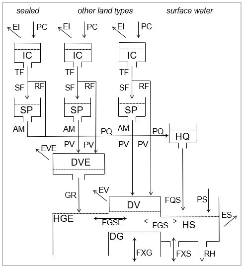
The following figure shows the general structure of wland_wag. Note that, besides
surface water areas and sealed surfaces, all land-use types rely on the same set of
process equations:
The WALRUS model defines some discontinuous differential equations, which
complicate numerical integration (Brauer et al., 2014). We applied the
regularisation techniques provided by the modules smoothutils and smoothtools
to remove these discontinuities. As shown for each equation (for example, in the
documentation on method Calc_RH_V1), this smoothing is optional. Set the related
parameters SH and ST to zero to disable smoothing so that the original WALRUS
relationships apply. The larger their values, the faster and more robust the
performance of the numerical integration algorithm, but the larger the discrepancies
to the discontinuous relationships. Our advice is to set small values like 1 mm or
1 °C (as in the following example calculations), respectively, which means that
there is no sharp transition from one behaviour to another at a certain threshold
but a smooth transition that mainly takes place in an interval of about 2 mm or 2 °C
around the threshold. As a consequence, a negative value for the amount of water
stored in the interception storage is acceptable, as the threshold of 0 mm does not
mean that the storage is completely empty but that two domains (the storage is empty
and the storage is not empty) are equally true (similar as in fuzzy logic).
Integration tests
Note
When new to HydPy, consider reading section Integration Tests first.
We perform all simulation runs over the same period of two months with a daily simulation step size:
>>> from hydpy import IntegrationTest, Element, pub, round_
>>> pub.timegrids = "2017-02-10", "2017-04-10", "1d"
wland_wag usually reads its temperature and precipitation input data from files and
receives its potential evaporation and evapotranspiration input data from a submodel
(petmodel), making the definition of the relevant Element object straightforward:
>>> from hydpy.models.wland_wag import *
>>> parameterstep("1d")
>>> land = Element("land", outlets="outlet")
>>> land.model = model
Our virtual test catchment has 10 km²:
>>> at(10.0)
We divide the land area into four hydrological response units of type FIELD,
CONIFER, SEALED and WATER (note that the first three land-related units are
optional, but the last water-related unit is required, as it corresponds to the surface
water storage, which is an integral component of the WALRUS concept):
>>> nu(4)
>>> lt(FIELD, CONIFER, SEALED, WATER)
In the first examples, we consider the catchment completely flat and hence define no hydrological response unit as “elevated”:
>>> er(False)
With the following setting, the water area is 0.2 km², so the total land area is 9.8 km². Of this, 0.98 km² are sealed, which makes the size of the (non-sealed) vadose zone 8.82 km²:
>>> aur(0.6 * 0.98, 0.3 * 0.98, 0.1 * 0.98, 0.02)
The lowland’s ground surface level is 1.5 m above sea level, and the channel bottom level is exactly at sea level, making a channel depth of 1.5 m:
>>> gl(1.5)
>>> bl(0.0)
The following parameter values lead to good results in a small catchment near the Kiel
Canal (northern part of Germany). For the parameter LAI, which provides land
use-specific values, we define only those values relevant for FIELD, CONIFER, and
SEALED. We adopt the default values for the “physical” soil parameters (B,
PsiAE, and ThetaS):
>>> cp(0.8)
>>> lai.sealed = 10.0
>>> lai.conifer = 11.0
>>> lai.field = 0.4, 0.4, 0.3, 0.7, 3.0, 5.2, 4.6, 3.1, 1.3, 0.2, 0.0, 0.0
>>> ih(0.2)
>>> tt(0.0)
>>> ti(4.0)
>>> ddf(5.0)
>>> ddt(0.0)
>>> cw(400.0)
>>> cv(0.2)
>>> cg(200000.0)
>>> cgf(1.0)
>>> cq(0.5)
>>> b(soil=SANDY_LOAM)
>>> psiae(soil=SANDY_LOAM)
>>> thetas(soil=SANDY_LOAM)
>>> zeta1(0.02)
>>> zeta2(400.0)
The elevated region parameters are not required for now, and we can set their values to
nan:
>>> cwe(nan)
>>> cge(nan)
>>> ac(nan)
We set both regularisation parameters to one (in agreement with the discussion above):
>>> sh(1.0)
>>> st(1.0)
In agreement with the original WALRUS model, we disable the RG option (the
documentation on method Calc_FGS_V1 explains the stabilising functionalities of the
restrictions RG is connected to) and the DGC option (we enable it in the
groundwater connect example):
>>> rg(False)
>>> dgc(False)
wland_wag requires a submodel for calculating the potential evapotranspiration of
land units and the potential evaporation of the sole water unit. We apply
evap_ret_io to smuggle in the underlying reference evapotranspiration.
evap_pet_mlc adjusts the given reference evapotranspiration to the month- and land
cover-specific potential evapotranspiration values:
>>> with model.add_petmodel_v1("evap_pet_mlc"):
...     landmonthfactor.sealed = 0.7
...     landmonthfactor.conifer = 1.3
...     landmonthfactor.field[1:4] = 0.73, 0.77, 0.95
...     landmonthfactor.water[1:4] = 1.22, 1.26, 1.28
...     dampingfactor(1.0)
...     with model.add_retmodel_v1("evap_ret_io"):
...         evapotranspirationfactor(0.9)
Additionally, wland_wag requires a submodel for calculating the discharge out of the
surface water storage (the same as the discharge at a catchment’s outlet. Here, we use
wq_walrus, which implements the default approach of the original WALRUS model:
>>> with model.add_dischargemodel_v2("wq_walrus"):
...     crestheight(0.0)
...     bankfulldischarge(8.0)
...     dischargeexponent(1.5)
Next, we initialise a test function object that prepares and runs the following tests and prints and plots their results:
>>> test = IntegrationTest(land)
All simulation runs start from dry conditions. The groundwater depth (DG, 1.6 m),
which is nearly in equilibrium with the water deficit in the vadose zone (DV, 0.14 m,
see method Calc_DVEq_V1), lies below the channel depth (CD, 1.5 m). The
interception height (IC), the snowpack (SP), and the surface water level (HS) are
intentionally negative to make sure even the regularised equations consider the related
storages as (almost) empty:
>>> test.inits = (
...     (states.ic, (-3.0, -3.0, -3.0, 0.0)),
...     (states.sp, (-3.0, -3.0, -3.0, 0.0)),
...     (states.dve, 140.0),
...     (states.dv, 140.0),
...     (states.hge, 900.0),
...     (states.dg, 1600.0),
...     (states.hq, 0.0),
...     (states.hs, -2.0),
...     (model.petmodel.sequences.logs.loggedpotentialevapotranspiration, 0.0),
... )
The following real data shows a shift from winter to spring conditions in the form of a rise in temperature and potential evapo(transpi)ration and includes two heavy rainfall events:
>>> inputs.t.series = (
...     -2.8, -1.5, -0.9, -1.6, -1.3, 1.7, 4.4, 4.5, 3.4, 4.8, 6.7, 5.8, 6.5, 5.0, 3.0,
...     3.1, 7.1, 9.4, 4.6, 3.7, 4.7, 5.9, 7.7, 6.3, 3.7, 1.6, 4.0, 5.6, 5.8, 5.7, 4.6,
...     4.2, 7.4, 6.3, 8.7, 6.4, 5.2, 5.1, 8.7, 6.2, 5.9, 5.2, 5.2, 5.9, 6.7, 7.0, 8.3,
...     9.0, 12.4, 15.0, 11.8, 9.4, 8.1, 7.9, 7.5, 7.2, 8.1, 8.6, 10.5)
>>> inputs.p.series = (
...     0.0, 0.4, 0.0, 0.0, 0.0, 0.0, 0.2, 4.5, 0.0, 3.2, 4.6, 2.3, 18.0, 19.2, 0.4,
...     8.3, 5.3, 0.7, 2.7, 1.6, 2.5, 0.6, 0.2, 1.7, 0.3, 0.0, 1.8, 8.9, 0.0, 0.0,
...     0.0, 0.9, 0.1, 0.0, 0.0, 3.9, 8.7, 26.4, 11.5, 0.9, 0.0, 0.0, 0.0, 0.0, 0.0,
...     0.0, 0.0, 1.5, 0.3, 0.2, 4.5, 0.0, 0.0, 0.0, 0.4, 0.0, 0.0, 0.0, 0.0)
>>> model.petmodel.retmodel.sequences.inputs.referenceevapotranspiration.series = (
...     0.6, 0.8, 0.7, 0.4, 0.4, 0.4, 0.4, 0.3, 0.3, 0.4, 0.3, 0.6, 0.8, 0.5, 0.8,
...     0.5, 0.4, 1.3, 0.9, 0.7, 0.7, 1.1, 1.0, 0.8, 0.6, 0.7, 0.7, 0.5, 0.8, 1.0,
...     1.2, 0.9, 0.9, 1.2, 1.4, 1.1, 1.1, 0.5, 0.6, 1.5, 2.0, 1.6, 1.6, 1.2, 1.3,
...     1.6, 1.9, 0.8, 1.5, 2.7, 1.5, 1.6, 2.0, 2.1, 1.7, 1.7, 0.8, 1.3, 2.5)
wland_wag allows for defining additional supply and extraction series. We will
discuss them later and set both to zero for now.
>>> inputs.fxg.series = 0.0
>>> inputs.fxs.series = 0.0
As we want to use method check_waterbalance() to prove that
wland_wag keeps the water balance in each example run, we need to store the defined
(initial) conditions before performing the first simulation run:
>>> test.reset_inits()
>>> conditions = model.conditions
base scenario
In our base scenario, we do not modify any of the settings described above. Initially, there is no exchange between groundwater and surface water due to the empty channel and the groundwater level below the channel bottom. The rainfall events increase both the groundwater level (via infiltration and percolation) and the surface water level (via quickflow generated on the sealed surfaces and on the saturated fraction of the vadose zone). Due to the faster rise of the surface water level, water first moves from the channel into groundwater (more concretely, it enters the vadose zone), but this inverses after the channel has discharged most of its content some days after the rainfall events.
>>> test("wland_wag_base_scenario",
... axis1=(fluxes.pc, fluxes.fqs, fluxes.fgs, fluxes.rh),
... axis2=(states.dg, states.hs))
Click to see the table
| date | t | p | fxg | fxs | dhs | pc | pe | pet | tf | ei | rf | sf | pm | am | ps | pve | pv | pq | etve | etv | es | et | gr | fxs | fxg | cdg | fgse | fgs | fqs | rh | r | ic | sp | dve | dv | hge | dg | hq | hs | outlet |
---------------------------------------------------------------------------------------------------------------------------------------------------------------------------------------------------------------------------------------------------------------------------------------------------------------------------------------------------------------------------------------------------------------------------------------------------------------------------------------------------------------------------------------------------------------------------------------------------------------------------------------------------------------------
| 2017-02-10 00:00:00 | -2.8 | 0.0 | 0.0 | 0.0 | 0.0 | 0.0 | 0.3942 0.702 0.378 0.6588 | 0.3942 0.702 0.378 0.0 | 0.0 0.0 0.0 0.0 | 0.0 0.000001 0.0 0.0 | 0.0 0.0 0.0 0.0 | 0.0 0.0 0.0 0.0 | 0.000117 0.000117 0.000117 0.0 | 0.0 0.0 0.0 0.0 | 0.0 | 0.0 | 0.0 | 0.0 | 0.0 | 0.49406 | 0.000066 | 0.435763 | 0.0 | 0.0 | 0.0 | 7.689815 | 0.0 | -0.000107 | 0.0 | 0.0 | 0.0 | -3.0 -3.000001 -3.0 0.0 | -3.0 -3.0 -3.0 0.0 | nan | 140.493953 | nan | 1607.689815 | 0.0 | -2.004788 | 0.0 |
| 2017-02-11 00:00:00 | -1.5 | 0.4 | 0.0 | 0.0 | 0.0 | 0.32 | 0.5256 0.936 0.504 0.8784 | 0.5256 0.936 0.504 0.0 | 0.000001 0.0 0.0 0.0 | 0.000001 0.000002 0.000001 0.0 | 0.0 0.0 0.0 0.0 | 0.0 0.0 0.0 0.0 | 0.009388 0.009388 0.009388 0.0 | 0.0 0.0 0.0 0.0 | 0.32 | 0.0 | 0.0 | 0.0 | 0.0 | 0.658704 | 0.000197 | 0.580983 | 0.0 | 0.0 | 0.0 | 5.794276 | 0.0 | -0.000114 | 0.0 | 0.0 | 0.0 | -2.680002 -2.680003 -2.680002 0.0 | -3.0 -3.0 -3.0 0.0 | nan | 141.152544 | nan | 1613.484091 | 0.0 | -1.690007 | 0.0 |
| 2017-02-12 00:00:00 | -0.9 | 0.0 | 0.0 | 0.0 | 0.0 | 0.0 | 0.4599 0.819 0.441 0.7686 | 0.4599 0.819 0.441 0.0 | 0.0 0.0 0.0 0.0 | 0.000002 0.000004 0.000002 0.0 | 0.0 0.0 0.0 0.0 | 0.0 0.0 0.0 0.0 | 0.069591 0.069591 0.069591 0.0 | 0.0 0.0 0.0 0.0 | 0.0 | 0.0 | 0.0 | 0.0 | 0.0 | 0.576325 | 0.000322 | 0.508328 | 0.0 | 0.0 | 0.0 | 4.967667 | 0.0 | -0.00012 | 0.0 | 0.0 | 0.0 | -2.680004 -2.680007 -2.680004 0.0 | -3.0 -3.0 -3.0 0.0 | nan | 141.728749 | nan | 1618.451759 | 0.0 | -1.695597 | 0.0 |
| 2017-02-13 00:00:00 | -1.6 | 0.0 | 0.0 | 0.0 | 0.0 | 0.0 | 0.2628 0.468 0.252 0.4392 | 0.2628 0.468 0.252 0.0 | 0.0 0.0 0.0 0.0 | 0.000001 0.000002 0.000001 0.0 | 0.0 0.0 0.0 0.0 | 0.0 0.0 0.0 0.0 | 0.006707 0.006707 0.006707 0.0 | 0.0 0.0 0.0 0.0 | 0.0 | 0.0 | 0.0 | 0.0 | 0.0 | 0.329312 | 0.000179 | 0.290458 | 0.0 | 0.0 | 0.0 | 3.946817 | 0.0 | -0.000124 | 0.0 | 0.0 | 0.0 | -2.680005 -2.680009 -2.680005 0.0 | -3.0 -3.0 -3.0 0.0 | nan | 142.057937 | nan | 1622.398575 | 0.0 | -1.70125 | 0.0 |
| 2017-02-14 00:00:00 | -1.3 | 0.0 | 0.0 | 0.0 | 0.0 | 0.0 | 0.2628 0.468 0.252 0.4392 | 0.2628 0.468 0.252 0.0 | 0.0 0.0 0.0 0.0 | 0.000001 0.000002 0.000001 0.0 | 0.0 0.0 0.0 0.0 | 0.0 0.0 0.0 0.0 | 0.018374 0.018374 0.018374 0.0 | 0.0 0.0 0.0 0.0 | 0.0 | 0.0 | 0.0 | 0.0 | 0.0 | 0.329299 | 0.000174 | 0.290447 | 0.0 | 0.0 | 0.0 | 3.067335 | 0.0 | -0.000128 | 0.0 | 0.0 | 0.0 | -2.680007 -2.680011 -2.680006 0.0 | -3.0 -3.0 -3.0 0.0 | nan | 142.387109 | nan | 1625.46591 | 0.0 | -1.707056 | 0.0 |
| 2017-02-15 00:00:00 | 1.7 | 0.0 | 0.0 | 0.0 | 0.0 | 0.0 | 0.2628 0.468 0.252 0.4392 | 0.2628 0.468 0.252 0.0 | 0.0 0.0 0.0 0.0 | 0.000001 0.000002 0.000001 0.0 | 0.0 0.0 0.0 0.0 | 0.0 0.0 0.0 0.0 | 8.50479 8.50479 8.50479 0.0 | 0.000009 0.000009 0.000009 0.0 | 0.0 | 0.0 | 0.000002 | 0.000007 | 0.0 | 0.329287 | 0.00017 | 0.290436 | 0.0 | 0.0 | 0.0 | 2.641574 | 0.0 | -0.000131 | 0.000004 | 0.0 | 0.0 | -2.680008 -2.680013 -2.680007 0.0 | -3.000008 -3.000009 -3.000009 0.0 | nan | 142.716262 | nan | 1628.107484 | 0.000002 | -1.712772 | 0.0 |
| 2017-02-16 00:00:00 | 4.4 | 0.2 | 0.0 | 0.0 | 0.0 | 0.16 | 0.2628 0.468 0.252 0.4392 | 0.2628 0.468 0.252 0.0 | 0.000001 0.0 0.0 0.0 | 0.000002 0.000003 0.000002 0.0 | 0.000001 0.0 0.0 0.0 | 0.0 0.0 0.0 0.0 | 22.000001 22.000001 22.000001 0.0 | 0.000023 0.000023 0.000023 0.0 | 0.16 | 0.0 | 0.000007 | 0.000017 | 0.0 | 0.329274 | 0.000244 | 0.290426 | 0.0 | 0.0 | 0.0 | 2.43789 | 0.0 | -0.000133 | 0.000013 | 0.0 | 0.0 | -2.52001 -2.520016 -2.520009 0.0 | -3.000031 -3.000032 -3.000032 0.0 | nan | 143.045396 | nan | 1630.545374 | 0.000007 | -1.558263 | 0.0 |
| 2017-02-17 00:00:00 | 4.5 | 4.5 | 0.0 | 0.0 | 0.0 | 3.6 | 0.1971 0.351 0.189 0.3294 | 0.1971 0.351 0.189 0.0 | 0.715908 0.000866 0.002554 0.0 | 0.045779 0.103421 0.056212 0.0 | 0.715908 0.000866 0.002554 0.0 | 0.0 0.0 0.0 0.0 | 22.5 22.5 22.5 0.0 | 0.000023 0.000023 0.000023 0.0 | 3.6 | 0.0 | 0.135679 | 0.307972 | 0.0 | 0.182336 | 0.18805 | 0.227414 | 0.0 | 0.0 | 0.0 | 2.022121 | 0.0 | -0.000783 | 0.080499 | 0.000245 | 0.000028 | 0.318303 0.975698 1.021225 0.0 | -3.000054 -3.000055 -3.000055 0.0 | nan | 143.09127 | nan | 1632.567495 | 0.227479 | 5.751347 | 0.000028 |
| 2017-02-18 00:00:00 | 3.4 | 0.0 | 0.0 | 0.0 | 0.0 | 0.0 | 0.1971 0.351 0.189 0.3294 | 0.1971 0.351 0.189 0.0 | 0.0 0.0 0.0 0.0 | 0.148001 0.341645 0.1863 0.0 | 0.0 0.0 0.0 0.0 | 0.0 0.0 0.0 0.0 | 17.000016 17.000016 17.000016 0.0 | 0.000018 0.000018 0.000018 0.0 | 0.0 | 0.0 | 0.000005 | 0.000013 | 0.0 | 0.035642 | 0.3294 | 0.24375 | 0.0 | 0.0 | 0.0 | 0.847145 | 0.0 | -0.008446 | 0.196805 | 0.005556 | 0.000643 | 0.170301 0.634053 0.834925 0.0 | -3.000072 -3.000072 -3.000072 0.0 | nan | 143.118461 | nan | 1633.41464 | 0.030687 | 14.415131 | 0.000643 |
| 2017-02-19 00:00:00 | 4.8 | 3.2 | 0.0 | 0.0 | 0.0 | 2.56 | 0.2628 0.468 0.252 0.4392 | 0.2628 0.468 0.252 0.0 | 2.024092 0.452925 0.899571 0.0 | 0.221756 0.46542 0.251473 0.0 | 2.024092 0.452925 0.899571 0.0 | 0.0 0.0 0.0 0.0 | 24.0 24.0 24.0 0.0 | 0.000025 0.000025 0.000025 0.0 | 2.56 | 0.0 | 0.425007 | 1.057808 | 0.0 | 0.028058 | 0.4392 | 0.325402 | 0.0 | 0.0 | 0.0 | -0.280715 | 0.0 | -0.020035 | 0.569784 | 0.017799 | 0.00206 | 0.484454 2.275708 2.243881 0.0 | -3.000097 -3.000097 -3.000097 0.0 | nan | 142.701477 | nan | 1633.133924 | 0.518711 | 42.681809 | 0.00206 |
| 2017-02-20 00:00:00 | 6.7 | 4.6 | 0.0 | 0.0 | 0.0 | 3.68 | 0.1971 0.351 0.189 0.3294 | 0.1971 0.351 0.189 0.0 | 3.340084 2.972153 3.208156 0.0 | 0.184112 0.350996 0.188997 0.0 | 3.340084 2.972153 3.208156 0.0 | 0.0 0.0 0.0 0.0 | 33.5 33.5 33.5 0.0 | 0.000035 0.000035 0.000035 0.0 | 3.68 | 0.0 | 0.90348 | 2.403414 | 0.0 | 0.00861 | 0.3294 | 0.244155 | 0.0 | 0.0 | 0.0 | -2.761647 | 0.0 | -0.087662 | 1.791561 | 0.101959 | 0.011801 | 0.640258 2.632559 2.526728 0.0 | -3.000131 -3.000131 -3.000131 0.0 | nan | 141.718945 | nan | 1630.372277 | 1.130565 | 124.855043 | 0.011801 |
| 2017-02-21 00:00:00 | 5.8 | 2.3 | 0.0 | 0.0 | 0.0 | 1.84 | 0.3942 0.702 0.378 0.6588 | 0.3942 0.702 0.378 0.0 | 1.642244 1.409245 1.61903 0.0 | 0.363824 0.701991 0.377995 0.0 | 1.642244 1.409245 1.61903 0.0 | 0.0 0.0 0.0 0.0 | 29.0 29.0 29.0 0.0 | 0.00003 0.00003 0.00003 0.0 | 1.84 | 0.0 | 0.434876 | 1.178664 | 0.0 | 0.02014 | 0.6588 | 0.488296 | 0.0 | 0.0 | 0.0 | -4.193367 | 0.0 | -0.229271 | 1.656831 | 0.276758 | 0.032032 | 0.47419 2.361323 2.369703 0.0 | -3.000161 -3.000161 -3.000161 0.0 | nan | 141.074938 | nan | 1626.178911 | 0.652398 | 183.272226 | 0.032032 |
| 2017-02-22 00:00:00 | 6.5 | 18.0 | 0.0 | 0.0 | 0.0 | 14.4 | 0.5256 0.936 0.504 0.8784 | 0.5256 0.936 0.504 0.0 | 13.589407 13.048734 13.564533 0.0 | 0.504696 0.935996 0.503997 0.0 | 13.589407 13.048734 13.564533 0.0 | 0.0 0.0 0.0 0.0 | 32.5 32.5 32.5 0.0 | 0.000033 0.000033 0.000033 0.0 | 14.4 | 0.0 | 3.615158 | 10.171109 | 0.0 | 0.013862 | 0.8784 | 0.65113 | 0.0 | 0.0 | 0.0 | -11.114303 | 0.0 | -0.625025 | 6.275288 | 0.697011 | 0.080673 | 0.780087 2.776593 2.701173 0.0 | -3.000194 -3.000195 -3.000195 0.0 | nan | 136.848616 | nan | 1615.064608 | 4.548219 | 441.86878 | 0.080673 |
| 2017-02-23 00:00:00 | 5.0 | 19.2 | 0.0 | 0.0 | 0.0 | 15.36 | 0.3285 0.585 0.315 0.549 | 0.3285 0.585 0.315 0.0 | 14.927283 14.658057 14.931707 0.0 | 0.322035 0.584999 0.314999 0.0 | 14.927283 14.658057 14.931707 0.0 | 0.0 0.0 0.0 0.0 | 25.0 25.0 25.0 0.0 | 0.000026 0.000026 0.000026 0.0 | 15.36 | 0.0 | 3.744198 | 11.477205 | 0.0 | 0.004289 | 0.549 | 0.406979 | 0.0 | 0.0 | 0.0 | -23.588977 | 0.0 | -2.217201 | 10.4167 | 2.091294 | 0.242048 | 0.890769 2.893537 2.814467 0.0 | -3.00022 -3.000221 -3.000221 0.0 | nan | 130.891507 | nan | 1591.475631 | 5.608724 | 764.754787 | 0.242048 |
| 2017-02-24 00:00:00 | 3.0 | 0.4 | 0.0 | 0.0 | 0.0 | 0.32 | 0.5256 0.936 0.504 0.8784 | 0.5256 0.936 0.504 0.0 | 0.294508 0.228149 0.294806 0.0 | 0.495653 0.935979 0.503995 0.0 | 0.294508 0.228149 0.294806 0.0 | 0.0 0.0 0.0 0.0 | 15.00006 15.00006 15.00006 0.0 | 0.000015 0.000015 0.000015 0.0 | 0.32 | 0.0 | 0.064376 | 0.216707 | 0.0 | 0.019884 | 0.8784 | 0.651119 | 0.0 | 0.0 | 0.0 | -28.145034 | 0.0 | -3.285909 | 4.977538 | 2.958151 | 0.342379 | 0.420607 2.049409 2.335665 0.0 | -3.000236 -3.000236 -3.000236 0.0 | nan | 127.561105 | nan | 1563.330597 | 0.847893 | 715.279595 | 0.342379 |
| 2017-02-25 00:00:00 | 3.1 | 8.3 | 0.0 | 0.0 | 0.0 | 6.64 | 0.3285 0.585 0.315 0.549 | 0.3285 0.585 0.315 0.0 | 6.067564 5.42086 6.057867 0.0 | 0.308297 0.584994 0.314997 0.0 | 6.067564 5.42086 6.057867 0.0 | 0.0 0.0 0.0 0.0 | 15.500043 15.500043 15.500043 0.0 | 0.000016 0.000016 0.000016 0.0 | 6.64 | 0.0 | 1.312185 | 4.691633 | 0.0 | 0.013415 | 0.549 | 0.406948 | 0.0 | 0.0 | 0.0 | -26.230308 | 0.0 | -2.432478 | 3.342513 | 2.402439 | 0.27806 | 0.684746 2.683555 2.602801 0.0 | -3.000251 -3.000252 -3.000252 0.0 | nan | 123.829857 | nan | 1537.100289 | 2.197013 | 657.75954 | 0.27806 |
| 2017-02-26 00:00:00 | 7.1 | 5.3 | 0.0 | 0.0 | 0.0 | 4.24 | 0.2628 0.468 0.252 0.4392 | 0.2628 0.468 0.252 0.0 | 3.990522 3.79688 3.989202 0.0 | 0.251896 0.467998 0.251998 0.0 | 3.990522 3.79688 3.989202 0.0 | 0.0 0.0 0.0 0.0 | 35.5 35.5 35.5 0.0 | 0.000037 0.000037 0.000037 0.0 | 4.24 | 0.0 | 0.838094 | 3.178049 | 0.0 | 0.007242 | 0.4392 | 0.325574 | 0.0 | 0.0 | 0.0 | -24.733905 | 0.0 | -2.179586 | 3.702601 | 2.271677 | 0.262926 | 0.682328 2.658677 2.601601 0.0 | -3.000288 -3.000288 -3.000288 0.0 | nan | 120.819419 | nan | 1512.366384 | 1.672461 | 633.284199 | 0.262926 |
| 2017-02-27 00:00:00 | 9.4 | 0.7 | 0.0 | 0.0 | 0.0 | 0.56 | 0.8541 1.521 0.819 1.4274 | 0.8541 1.521 0.819 0.0 | 0.424006 0.206871 0.404319 0.0 | 0.69546 1.52066 0.818961 0.0 | 0.424006 0.206871 0.404319 0.0 | 0.0 0.0 0.0 0.0 | 47.0 47.0 47.0 0.0 | 0.000048 0.000048 0.000048 0.0 | 0.56 | 0.0 | 0.072506 | 0.29169 | 0.0 | 0.105486 | 1.4274 | 1.05785 | 0.0 | 0.0 | 0.0 | -20.541689 | 0.0 | -1.75328 | 1.629416 | 1.977757 | 0.228907 | 0.122863 1.491146 1.93832 0.0 | -3.000336 -3.000337 -3.000337 0.0 | nan | 119.099119 | nan | 1491.824695 | 0.334735 | 536.050645 | 0.228907 |
| 2017-02-28 00:00:00 | 4.6 | 2.7 | 0.0 | 0.0 | 0.0 | 2.16 | 0.5913 1.053 0.567 0.9882 | 0.5913 1.053 0.567 0.0 | 1.503577 0.475598 1.340285 0.0 | 0.453541 1.052728 0.566963 0.0 | 1.503577 0.475598 1.340285 0.0 | 0.0 0.0 0.0 0.0 | 23.0 23.0 23.0 0.0 | 0.000024 0.000024 0.000024 0.0 | 2.16 | 0.0 | 0.233307 | 0.968901 | 0.0 | 0.091601 | 0.9882 | 0.732303 | 0.0 | 0.0 | 0.0 | -15.277137 | 0.0 | -1.159541 | 0.810665 | 1.490405 | 0.172501 | 0.325745 2.122819 2.191072 0.0 | -3.00036 -3.000361 -3.000361 0.0 | nan | 117.797872 | nan | 1476.547558 | 0.492971 | 451.289017 | 0.172501 |
| 2017-03-01 00:00:00 | 3.7 | 1.6 | 0.0 | 0.0 | 0.0 | 1.28 | 0.4851 0.819 0.441 0.7938 | 0.4851 0.819 0.441 0.0 | 0.950974 0.496744 0.876127 0.0 | 0.384181 0.818947 0.440979 0.0 | 0.950974 0.496744 0.876127 0.0 | 0.0 0.0 0.0 0.0 | 18.500006 18.500006 18.500006 0.0 | 0.000019 0.000019 0.000019 0.0 | 1.28 | 0.0 | 0.158043 | 0.665001 | 0.0 | 0.067062 | 0.7938 | 0.58491 | 0.0 | 0.0 | 0.0 | -11.475157 | 0.0 | -0.83105 | 0.805046 | 1.195722 | 0.138394 | 0.27059 2.087128 2.153966 0.0 | -3.000379 -3.00038 -3.00038 0.0 | nan | 116.875841 | nan | 1465.0724 | 0.352927 | 394.787074 | 0.138394 |
| 2017-03-02 00:00:00 | 4.7 | 2.5 | 0.0 | 0.0 | 0.0 | 2.0 | 0.4851 0.819 0.441 0.7938 | 0.4851 0.819 0.441 0.0 | 1.532391 1.007088 1.460286 0.0 | 0.393841 0.818966 0.440983 0.0 | 1.532391 1.007088 1.460286 0.0 | 0.0 0.0 0.0 0.0 | 23.5 23.5 23.5 0.0 | 0.000024 0.000024 0.000024 0.0 | 2.0 | 0.0 | 0.264558 | 1.129511 | 0.0 | 0.060642 | 0.7938 | 0.584933 | 0.0 | 0.0 | 0.0 | -8.783965 | 0.0 | -0.635253 | 0.937585 | 1.006555 | 0.116499 | 0.344358 2.261073 2.252696 0.0 | -3.000403 -3.000404 -3.000404 0.0 | nan | 116.036672 | nan | 1456.288435 | 0.544853 | 363.592537 | 0.116499 |
| 2017-03-03 00:00:00 | 5.9 | 0.6 | 0.0 | 0.0 | 0.0 | 0.48 | 0.7623 1.287 0.693 1.2474 | 0.7623 1.287 0.693 0.0 | 0.289055 0.089404 0.242334 0.0 | 0.506024 1.286381 0.692918 0.0 | 0.289055 0.089404 0.242334 0.0 | 0.0 0.0 0.0 0.0 | 29.5 29.5 29.5 0.0 | 0.00003 0.00003 0.00003 0.0 | 0.48 | 0.0 | 0.042962 | 0.185852 | 0.0 | 0.170478 | 1.2474 | 0.918953 | 0.0 | 0.0 | 0.0 | -6.560051 | 0.0 | -0.517507 | 0.588667 | 0.886421 | 0.102595 | 0.029279 1.365288 1.797444 0.0 | -3.000434 -3.000434 -3.000434 0.0 | nan | 115.646681 | nan | 1449.728383 | 0.142038 | 324.526695 | 0.102595 |
| 2017-03-04 00:00:00 | 7.7 | 0.2 | 0.0 | 0.0 | 0.0 | 0.16 | 0.693 1.17 0.63 1.134 | 0.693 1.17 0.63 0.0 | 0.056033 0.000734 0.020474 0.0 | 0.287113 1.129003 0.629377 0.0 | 0.056033 0.000734 0.020474 0.0 | 0.0 0.0 0.0 0.0 | 38.5 38.5 38.5 0.0 | 0.00004 0.00004 0.00004 0.0 | 0.16 | 0.0 | 0.007236 | 0.029414 | 0.0 | 0.283298 | 1.134 | 0.834977 | 0.0 | 0.0 | 0.0 | -4.06809 | 0.0 | -0.37469 | 0.141336 | 0.719279 | 0.08325 | -0.153866 0.395551 1.307593 0.0 | -3.000473 -3.000474 -3.000474 0.0 | nan | 115.548053 | nan | 1445.660293 | 0.030116 | 277.990378 | 0.08325 |
| 2017-03-05 00:00:00 | 6.3 | 1.7 | 0.0 | 0.0 | 0.0 | 1.36 | 0.5544 0.936 0.504 0.9072 | 0.5544 0.936 0.504 0.0 | 0.697906 0.001281 0.262456 0.0 | 0.32067 0.881557 0.50364 0.0 | 0.697906 0.001281 0.262456 0.0 | 0.0 0.0 0.0 0.0 | 31.5 31.5 31.5 0.0 | 0.000032 0.000032 0.000032 0.0 | 1.36 | 0.0 | 0.089357 | 0.364984 | 0.0 | 0.173382 | 0.9072 | 0.668155 | 0.0 | 0.0 | 0.0 | -2.430955 | 0.0 | -0.268696 | 0.21477 | 0.58127 | 0.067277 | 0.187557 0.872714 1.901496 0.0 | -3.000506 -3.000506 -3.000506 0.0 | nan | 115.363382 | nan | 1443.229338 | 0.180331 | 248.053934 | 0.067277 |
| 2017-03-06 00:00:00 | 3.7 | 0.3 | 0.0 | 0.0 | 0.0 | 0.24 | 0.4158 0.702 0.378 0.6804 | 0.4158 0.702 0.378 0.0 | 0.132096 0.000231 0.068033 0.0 | 0.256414 0.66439 0.377897 0.0 | 0.132096 0.000231 0.068033 0.0 | 0.0 0.0 0.0 0.0 | 18.500006 18.500006 18.500006 0.0 | 0.000019 0.000019 0.000019 0.0 | 0.24 | 0.0 | 0.016872 | 0.070964 | 0.0 | 0.118396 | 0.6804 | 0.501169 | 0.0 | 0.0 | 0.0 | -1.80417 | 0.0 | -0.210597 | 0.198459 | 0.49936 | 0.057796 | 0.039047 0.448093 1.695566 0.0 | -3.000525 -3.000525 -3.000525 0.0 | nan | 115.254309 | nan | 1441.425168 | 0.052836 | 223.0827 | 0.057796 |
| 2017-03-07 00:00:00 | 1.6 | 0.0 | 0.0 | 0.0 | 0.0 | 0.0 | 0.4851 0.819 0.441 0.7938 | 0.4851 0.819 0.441 0.0 | 0.0 0.0 0.0 0.0 | 0.203547 0.529923 0.440409 0.0 | 0.0 0.0 0.0 0.0 | 0.0 0.0 0.0 0.0 | 8.006707 8.006707 8.006707 0.0 | 0.000008 0.000008 0.000008 0.0 | 0.0 | 0.0 | 0.000002 | 0.000007 | 0.0 | 0.283108 | 0.7938 | 0.58422 | 0.0 | 0.0 | 0.0 | -0.861878 | 0.0 | -0.158245 | 0.044621 | 0.418457 | 0.048432 | -0.1645 -0.08183 1.255157 0.0 | -3.000533 -3.000533 -3.000533 0.0 | nan | 115.37917 | nan | 1440.56329 | 0.008222 | 196.57392 | 0.048432 |
| 2017-03-08 00:00:00 | 4.0 | 1.8 | 0.0 | 0.0 | 0.0 | 1.44 | 0.4851 0.819 0.441 0.7938 | 0.4851 0.819 0.441 0.0 | 0.768023 0.000465 0.300985 0.0 | 0.289705 0.646837 0.440659 0.0 | 0.768023 0.000465 0.300985 0.0 | 0.0 0.0 0.0 0.0 | 20.000002 20.000002 20.000002 0.0 | 0.000021 0.000021 0.000021 0.0 | 1.44 | 0.0 | 0.098161 | 0.402728 | 0.0 | 0.18702 | 0.7938 | 0.584529 | 0.0 | 0.0 | 0.0 | -0.128107 | 0.0 | -0.12201 | 0.213834 | 0.357061 | 0.041327 | 0.217772 0.710868 1.953512 0.0 | -3.000553 -3.000554 -3.000554 0.0 | nan | 115.34602 | nan | 1440.435182 | 0.197116 | 184.464299 | 0.041327 |
| 2017-03-09 00:00:00 | 5.6 | 8.9 | 0.0 | 0.0 | 0.0 | 7.12 | 0.3465 0.585 0.315 0.567 | 0.3465 0.585 0.315 0.0 | 6.358222 4.564114 6.159931 0.0 | 0.317377 0.584263 0.314994 0.0 | 6.358222 4.564114 6.159931 0.0 | 0.0 0.0 0.0 0.0 | 28.0 28.0 28.0 0.0 | 0.000029 0.000029 0.000029 0.0 | 7.12 | 0.0 | 1.092232 | 4.81718 | 0.0 | 0.019596 | 0.567 | 0.417884 | 0.0 | 0.0 | 0.0 | -2.500922 | 0.0 | -0.188908 | 2.755409 | 0.465767 | 0.053908 | 0.662173 2.682491 2.598587 0.0 | -3.000582 -3.000583 -3.000583 0.0 | nan | 114.084476 | nan | 1437.934261 | 2.258887 | 294.413161 | 0.053908 |
| 2017-03-10 00:00:00 | 5.8 | 0.0 | 0.0 | 0.0 | 0.0 | 0.0 | 0.5544 0.936 0.504 0.9072 | 0.5544 0.936 0.504 0.0 | 0.0 0.0 0.0 0.0 | 0.47338 0.93593 0.503987 0.0 | 0.0 0.0 0.0 0.0 | 0.0 0.0 0.0 0.0 | 29.0 29.0 29.0 0.0 | 0.00003 0.00003 0.00003 0.0 | 0.0 | 0.0 | 0.000006 | 0.000025 | 0.0 | 0.053861 | 0.9072 | 0.668551 | 0.0 | 0.0 | 0.0 | -4.26993 | 0.0 | -0.431726 | 1.953076 | 0.816723 | 0.094528 | 0.188793 1.746561 2.0946 0.0 | -3.000612 -3.000612 -3.000612 0.0 | nan | 113.706605 | nan | 1433.664331 | 0.305836 | 329.331417 | 0.094528 |
| 2017-03-11 00:00:00 | 5.7 | 0.0 | 0.0 | 0.0 | 0.0 | 0.0 | 0.693 1.17 0.63 1.134 | 0.693 1.17 0.63 0.0 | 0.0 0.0 0.0 0.0 | 0.342789 1.155723 0.629755 0.0 | 0.0 0.0 0.0 0.0 | 0.0 0.0 0.0 0.0 | 28.5 28.5 28.5 0.0 | 0.000029 0.000029 0.000029 0.0 | 0.0 | 0.0 | 0.000005 | 0.000024 | 0.0 | 0.23746 | 1.134 | 0.835178 | 0.0 | 0.0 | 0.0 | -3.094948 | 0.0 | -0.373701 | 0.2646 | 0.749147 | 0.086707 | -0.153996 0.590838 1.464845 0.0 | -3.000641 -3.000642 -3.000642 0.0 | nan | 113.570358 | nan | 1430.569383 | 0.041261 | 287.225184 | 0.086707 |
| 2017-03-12 00:00:00 | 4.6 | 0.0 | 0.0 | 0.0 | 0.0 | 0.0 | 0.8316 1.404 0.756 1.3608 | 0.8316 1.404 0.756 0.0 | 0.0 0.0 0.0 0.0 | 0.194383 0.816565 0.748178 0.0 | 0.0 0.0 0.0 0.0 | 0.0 0.0 0.0 0.0 | 23.0 23.0 23.0 0.0 | 0.000024 0.000024 0.000024 0.0 | 0.0 | 0.0 | 0.000004 | 0.00002 | 0.0 | 0.618605 | 1.3608 | 1.000515 | 0.0 | 0.0 | 0.0 | -1.103459 | 0.0 | -0.261297 | 0.034854 | 0.598105 | 0.069225 | -0.348379 -0.225728 0.716667 0.0 | -3.000665 -3.000665 -3.000665 0.0 | nan | 113.927662 | nan | 1429.465924 | 0.006427 | 246.14379 | 0.069225 |
| 2017-03-13 00:00:00 | 4.2 | 0.9 | 0.0 | 0.0 | 0.0 | 0.72 | 0.6237 1.053 0.567 1.0206 | 0.6237 1.053 0.567 0.0 | 0.198229 0.000023 0.002956 0.0 | 0.206806 0.450434 0.55268 0.0 | 0.198229 0.000023 0.002956 0.0 | 0.0 0.0 0.0 0.0 | 21.000001 21.000001 21.000001 0.0 | 0.000022 0.000022 0.000022 0.0 | 0.72 | 0.0 | 0.024808 | 0.096934 | 0.0 | 0.477218 | 1.0206 | 0.74951 | 0.0 | 0.0 | 0.0 | 0.763914 | 0.0 | -0.184622 | 0.054332 | 0.481406 | 0.055718 | -0.033414 0.043816 0.88103 0.0 | -3.000687 -3.000687 -3.000687 0.0 | nan | 114.195449 | nan | 1430.229837 | 0.049028 | 216.29334 | 0.055718 |
| 2017-03-14 00:00:00 | 7.4 | 0.1 | 0.0 | 0.0 | 0.0 | 0.08 | 0.6237 1.053 0.567 1.0206 | 0.6237 1.053 0.567 0.0 | 0.023925 0.000002 0.000192 0.0 | 0.224 0.377245 0.535208 0.0 | 0.023925 0.000002 0.000192 0.0 | 0.0 0.0 0.0 0.0 | 37.0 37.0 37.0 0.0 | 0.000038 0.000038 0.000038 0.0 | 0.08 | 0.0 | 0.003012 | 0.011701 | 0.0 | 0.490099 | 1.0206 | 0.747752 | 0.0 | 0.0 | 0.0 | 1.391522 | 0.0 | -0.13748 | 0.049666 | 0.400871 | 0.046397 | -0.201339 -0.253432 0.42563 0.0 | -3.000725 -3.000725 -3.000725 0.0 | nan | 114.545056 | nan | 1431.621359 | 0.011064 | 191.679973 | 0.046397 |
| 2017-03-15 00:00:00 | 6.3 | 0.0 | 0.0 | 0.0 | 0.0 | 0.0 | 0.8316 1.404 0.756 1.3608 | 0.8316 1.404 0.756 0.0 | 0.0 0.0 0.0 0.0 | 0.171792 0.216402 0.491988 0.0 | 0.0 0.0 0.0 0.0 | 0.0 0.0 0.0 0.0 | 31.5 31.5 31.5 0.0 | 0.000032 0.000032 0.000032 0.0 | 0.0 | 0.0 | 0.000006 | 0.000027 | 0.0 | 0.832956 | 1.3608 | 0.974734 | 0.0 | 0.0 | 0.0 | 2.737916 | 0.0 | -0.102217 | 0.01034 | 0.333613 | 0.038613 | -0.373131 -0.469834 -0.066358 0.0 | -3.000757 -3.000757 -3.000757 0.0 | nan | 115.275789 | nan | 1434.359276 | 0.00075 | 169.637443 | 0.038613 |
| 2017-03-16 00:00:00 | 8.7 | 0.0 | 0.0 | 0.0 | 0.0 | 0.0 | 0.9702 1.638 0.882 1.5876 | 0.9702 1.638 0.882 0.0 | 0.0 0.0 0.0 0.0 | 0.1163 0.128043 0.249226 0.0 | 0.0 0.0 0.0 0.0 | 0.0 0.0 0.0 0.0 | 43.5 43.5 43.5 0.0 | 0.000045 0.000045 0.000045 0.0 | 0.0 | 0.0 | 0.000009 | 0.000037 | 0.0 | 1.068953 | 1.5876 | 1.105022 | 0.0 | 0.0 | 0.0 | 4.549635 | 0.0 | -0.077193 | 0.00072 | 0.278598 | 0.032245 | -0.489431 -0.597877 -0.315584 0.0 | -3.000802 -3.000802 -3.000802 0.0 | nan | 116.267541 | nan | 1438.90891 | 0.000067 | 150.751015 | 0.032245 |
| 2017-03-17 00:00:00 | 6.4 | 3.9 | 0.0 | 0.0 | 0.0 | 3.12 | 0.7623 1.287 0.693 1.2474 | 0.7623 1.287 0.693 0.0 | 1.81828 0.016202 0.251066 0.0 | 0.484927 0.98936 0.602563 0.0 | 1.81828 0.016202 0.251066 0.0 | 0.0 0.0 0.0 0.0 | 32.0 32.0 32.0 0.0 | 0.000033 0.000033 0.000033 0.0 | 3.12 | 0.0 | 0.236941 | 0.907721 | 0.0 | 0.283155 | 1.2474 | 0.909751 | 0.0 | 0.0 | 0.0 | 4.115983 | 0.0 | -0.069315 | 0.445455 | 0.254748 | 0.029485 | 0.327362 1.516561 1.950786 0.0 | -3.000834 -3.000835 -3.000835 0.0 | nan | 116.244441 | nan | 1443.024893 | 0.462333 | 158.656741 | 0.029485 |
| 2017-03-18 00:00:00 | 5.2 | 8.7 | 0.0 | 0.0 | 0.0 | 6.96 | 0.7623 1.287 0.693 1.2474 | 0.7623 1.287 0.693 0.0 | 6.071917 4.671897 5.753546 0.0 | 0.686 1.286933 0.692984 0.0 | 6.071917 4.671897 5.753546 0.0 | 0.0 0.0 0.0 0.0 | 26.0 26.0 26.0 0.0 | 0.000027 0.000027 0.000027 0.0 | 6.96 | 0.0 | 1.079093 | 4.648917 | 0.0 | 0.050717 | 1.2474 | 0.919319 | 0.0 | 0.0 | 0.0 | -0.494838 | 0.0 | -0.164085 | 2.95231 | 0.417922 | 0.048371 | 0.529445 2.517732 2.464257 0.0 | -3.000861 -3.000862 -3.000862 0.0 | nan | 115.051979 | nan | 1442.530055 | 2.15894 | 280.900255 | 0.048371 |
| 2017-03-19 00:00:00 | 5.1 | 26.4 | 0.0 | 0.0 | 0.0 | 21.12 | 0.3465 0.585 0.315 0.567 | 0.3465 0.585 0.315 0.0 | 20.402677 20.093743 20.41012 0.0 | 0.337473 0.584999 0.314999 0.0 | 20.402677 20.093743 20.41012 0.0 | 0.0 0.0 0.0 0.0 | 25.5 25.5 25.5 0.0 | 0.000026 0.000026 0.000026 0.0 | 21.12 | 0.0 | 3.729056 | 16.954617 | 0.0 | 0.005999 | 0.567 | 0.417925 | 0.0 | 0.0 | 0.0 | -11.38646 | 0.0 | -1.107128 | 11.413765 | 1.503708 | 0.17404 | 0.909295 2.95899 2.859138 0.0 | -3.000887 -3.000888 -3.000888 0.0 | nan | 110.221794 | nan | 1431.143595 | 7.699791 | 736.718013 | 0.17404 |
| 2017-03-20 00:00:00 | 8.7 | 11.5 | 0.0 | 0.0 | 0.0 | 9.2 | 0.4158 0.702 0.378 0.6804 | 0.4158 0.702 0.378 0.0 | 8.931919 8.697378 8.951398 0.0 | 0.406536 0.701998 0.377999 0.0 | 8.931919 8.697378 8.951398 0.0 | 0.0 0.0 0.0 0.0 | 43.5 43.5 43.5 0.0 | 0.000045 0.000045 0.000045 0.0 | 9.2 | 0.0 | 1.49534 | 7.517743 | 0.0 | 0.006158 | 0.6804 | 0.501515 | 0.0 | 0.0 | 0.0 | -23.730355 | 0.0 | -3.519331 | 10.929521 | 3.589164 | 0.415413 | 0.77084 2.759614 2.729741 0.0 | -3.000932 -3.000932 -3.000932 0.0 | nan | 105.21328 | nan | 1407.41324 | 4.288012 | 946.123457 | 0.415413 |
| 2017-03-21 00:00:00 | 6.2 | 0.9 | 0.0 | 0.0 | 0.0 | 0.72 | 1.0395 1.755 0.945 1.701 | 1.0395 1.755 0.945 0.0 | 0.554074 0.276005 0.54812 0.0 | 0.842801 1.754558 0.944963 0.0 | 0.554074 0.276005 0.54812 0.0 | 0.0 0.0 0.0 0.0 | 31.0 31.0 31.0 0.0 | 0.000032 0.000032 0.000032 0.0 | 0.72 | 0.0 | 0.072301 | 0.405019 | 0.0 | 0.130937 | 1.701 | 1.25352 | 0.0 | 0.0 | 0.0 | -27.828005 | 0.0 | -3.512382 | 3.963595 | 3.670279 | 0.424801 | 0.093965 1.449051 1.956658 0.0 | -3.000964 -3.000964 -3.000964 0.0 | nan | 101.759535 | nan | 1379.585235 | 0.729437 | 800.94858 | 0.424801 |
| 2017-03-22 00:00:00 | 5.9 | 0.0 | 0.0 | 0.0 | 0.0 | 0.0 | 1.386 2.34 1.26 2.268 | 1.386 2.34 1.26 0.0 | 0.0 0.0 0.0 0.0 | 0.443436 1.687914 1.251505 0.0 | 0.0 0.0 0.0 0.0 | 0.0 0.0 0.0 0.0 | 29.5 29.5 29.5 0.0 | 0.00003 0.00003 0.00003 0.0 | 0.0 | 0.0 | 0.000005 | 0.000026 | 0.0 | 0.843611 | 2.268 | 1.669059 | 0.0 | 0.0 | 0.0 | -22.152341 | 0.0 | -2.018508 | 0.630772 | 2.568823 | 0.297317 | -0.349471 -0.238864 0.705152 0.0 | -3.000994 -3.000994 -3.000994 0.0 | nan | 100.584634 | nan | 1357.432894 | 0.098691 | 612.131103 | 0.297317 |
| 2017-03-23 00:00:00 | 5.2 | 0.0 | 0.0 | 0.0 | 0.0 | 0.0 | 1.1088 1.872 1.008 1.8144 | 1.1088 1.872 1.008 0.0 | 0.0 0.0 0.0 0.0 | 0.139041 0.269899 0.749339 0.0 | 0.0 0.0 0.0 0.0 | 0.0 0.0 0.0 0.0 | 26.0 26.0 26.0 0.0 | 0.000027 0.000027 0.000027 0.0 | 0.0 | 0.0 | 0.000004 | 0.000023 | 0.0 | 1.177587 | 1.8144 | 1.309461 | 0.0 | 0.0 | 0.0 | -12.450409 | 0.0 | -1.070944 | 0.083352 | 1.740289 | 0.201422 | -0.488513 -0.508763 -0.044186 0.0 | -3.001021 -3.001021 -3.001021 0.0 | nan | 100.691273 | nan | 1344.982485 | 0.015362 | 480.157885 | 0.201422 |
| 2017-03-24 00:00:00 | 5.2 | 0.0 | 0.0 | 0.0 | 0.0 | 0.0 | 1.1088 1.872 1.008 1.8144 | 1.1088 1.872 1.008 0.0 | 0.0 0.0 0.0 0.0 | 0.087814 0.124874 0.28534 0.0 | 0.0 0.0 0.0 0.0 | 0.0 0.0 0.0 0.0 | 26.0 26.0 26.0 0.0 | 0.000027 0.000027 0.000027 0.0 | 0.0 | 0.0 | 0.000004 | 0.000023 | 0.0 | 1.259847 | 1.8144 | 1.263784 | 0.0 | 0.0 | 0.0 | -4.704504 | 0.0 | -0.59793 | 0.012985 | 1.241013 | 0.143636 | -0.576326 -0.633637 -0.329527 0.0 | -3.001047 -3.001048 -3.001048 0.0 | nan | 101.353186 | nan | 1340.277981 | 0.002399 | 390.560405 | 0.143636 |
| 2017-03-25 00:00:00 | 5.9 | 0.0 | 0.0 | 0.0 | 0.0 | 0.0 | 0.8316 1.404 0.756 1.3608 | 0.8316 1.404 0.756 0.0 | 0.0 0.0 0.0 0.0 | 0.049326 0.062903 0.10945 0.0 | 0.0 0.0 0.0 0.0 | 0.0 0.0 0.0 0.0 | 29.5 29.5 29.5 0.0 | 0.00003 0.00003 0.00003 0.0 | 0.0 | 0.0 | 0.000005 | 0.000026 | 0.0 | 0.966074 | 1.3608 | 0.937516 | 0.0 | 0.0 | 0.0 | -0.037149 | 0.0 | -0.353877 | 0.002253 | 0.930564 | 0.107704 | -0.625652 -0.696541 -0.438977 0.0 | -3.001078 -3.001078 -3.001078 0.0 | nan | 101.965379 | nan | 1340.240832 | 0.000172 | 327.175886 | 0.107704 |
| 2017-03-26 00:00:00 | 6.7 | 0.0 | 0.0 | 0.0 | 0.0 | 0.0 | 0.9009 1.521 0.819 1.4742 | 0.9009 1.521 0.819 0.0 | 0.0 0.0 0.0 0.0 | 0.043673 0.052838 0.08103 0.0 | 0.0 0.0 0.0 0.0 | 0.0 0.0 0.0 0.0 | 33.5 33.5 33.5 0.0 | 0.000034 0.000034 0.000034 0.0 | 0.0 | 0.0 | 0.000005 | 0.00003 | 0.0 | 1.058121 | 1.4742 | 1.011902 | 0.0 | 0.0 | 0.0 | 2.691376 | 0.0 | -0.218352 | 0.000176 | 0.724801 | 0.083889 | -0.669325 -0.749379 -0.520006 0.0 | -3.001112 -3.001112 -3.001112 0.0 | nan | 102.805143 | nan | 1342.932208 | 0.000025 | 279.840973 | 0.083889 |
| 2017-03-27 00:00:00 | 7.0 | 0.0 | 0.0 | 0.0 | 0.0 | 0.0 | 1.1088 1.872 1.008 1.8144 | 1.1088 1.872 1.008 0.0 | 0.0 0.0 0.0 0.0 | 0.044305 0.051551 0.072316 0.0 | 0.0 0.0 0.0 0.0 | 0.0 0.0 0.0 0.0 | 35.0 35.0 35.0 0.0 | 0.000036 0.000036 0.000036 0.0 | 0.0 | 0.0 | 0.000006 | 0.000031 | 0.0 | 1.312997 | 1.8144 | 1.242646 | 0.0 | 0.0 | 0.0 | 5.113689 | 0.0 | -0.138549 | 0.00004 | 0.579836 | 0.067111 | -0.713631 -0.80093 -0.592322 0.0 | -3.001148 -3.001148 -3.001148 0.0 | nan | 103.979585 | nan | 1348.045897 | 0.000016 | 242.9267 | 0.067111 |
| 2017-03-28 00:00:00 | 8.3 | 0.0 | 0.0 | 0.0 | 0.0 | 0.0 | 1.3167 2.223 1.197 2.1546 | 1.3167 2.223 1.197 0.0 | 0.0 0.0 0.0 0.0 | 0.043336 0.04889 0.064069 0.0 | 0.0 0.0 0.0 0.0 | 0.0 0.0 0.0 0.0 | 41.5 41.5 41.5 0.0 | 0.000043 0.000043 0.000043 0.0 | 0.0 | 0.0 | 0.000007 | 0.000036 | 0.0 | 1.569338 | 2.1546 | 1.473382 | 0.0 | 0.0 | 0.0 | 7.493869 | 0.0 | -0.090279 | 0.000034 | 0.472829 | 0.054726 | -0.756967 -0.84982 -0.656391 0.0 | -3.00119 -3.001191 -3.001191 0.0 | nan | 105.458637 | nan | 1355.539767 | 0.000018 | 213.151032 | 0.054726 |
| 2017-03-29 00:00:00 | 9.0 | 1.5 | 0.0 | 0.0 | 0.0 | 1.2 | 0.5544 0.936 0.504 0.9072 | 0.5544 0.936 0.504 0.0 | 0.260717 0.000022 0.000145 0.0 | 0.144525 0.238019 0.204298 0.0 | 0.260717 0.000022 0.000145 0.0 | 0.0 0.0 0.0 0.0 | 45.0 45.0 45.0 0.0 | 0.000046 0.000046 0.000046 0.0 | 1.2 | 0.0 | 0.028316 | 0.131013 | 0.0 | 0.504509 | 0.9072 | 0.638101 | 0.0 | 0.0 | 0.0 | 7.180132 | 0.0 | -0.062559 | 0.054688 | 0.396534 | 0.045895 | 0.037791 0.112138 0.339166 0.0 | -3.001236 -3.001237 -3.001237 0.0 | nan | 105.872271 | nan | 1362.719899 | 0.076343 | 193.537988 | 0.045895 |
| 2017-03-30 00:00:00 | 12.4 | 0.3 | 0.0 | 0.0 | 0.0 | 0.24 | 1.0395 1.755 0.945 1.701 | 1.0395 1.755 0.945 0.0 | 0.077209 0.000006 0.00005 0.0 | 0.398283 0.624966 0.601961 0.0 | 0.077209 0.000006 0.00005 0.0 | 0.0 0.0 0.0 0.0 | 62.0 62.0 62.0 0.0 | 0.000064 0.000064 0.000064 0.0 | 0.24 | 0.0 | 0.008451 | 0.03879 | 0.0 | 0.801904 | 1.701 | 1.218222 | 0.0 | 0.0 | 0.0 | 5.557628 | 0.0 | -0.047286 | 0.089824 | 0.347786 | 0.040253 | -0.197701 -0.272834 -0.022845 0.0 | -3.0013 -3.0013 -3.0013 0.0 | nan | 106.618438 | nan | 1368.277527 | 0.025309 | 177.003752 | 0.040253 |
| 2017-03-31 00:00:00 | 15.0 | 0.2 | 0.0 | 0.0 | 0.0 | 0.16 | 1.8711 3.159 1.701 3.0618 | 1.8711 3.159 1.701 0.0 | 0.023655 0.000001 0.000007 0.0 | 0.347261 0.40353 0.470752 0.0 | 0.023655 0.000001 0.000007 0.0 | 0.0 0.0 0.0 0.0 | 75.0 75.0 75.0 0.0 | 0.000077 0.000077 0.000077 0.0 | 0.16 | 0.0 | 0.002656 | 0.01188 | 0.0 | 1.92882 | 3.0618 | 2.131417 | 0.0 | 0.0 | 0.0 | 7.863292 | 0.0 | -0.033495 | 0.028937 | 0.299798 | 0.034699 | -0.408618 -0.516365 -0.333604 0.0 | -3.001377 -3.001377 -3.001377 0.0 | nan | 108.511108 | nan | 1376.140819 | 0.008252 | 159.052854 | 0.034699 |
| 2017-04-01 00:00:00 | 11.8 | 4.5 | 0.0 | 0.0 | 0.0 | 3.6 | 1.2825 1.755 0.945 1.728 | 1.2825 1.755 0.945 0.0 | 1.991939 0.031211 0.413616 0.0 | 0.874746 1.4273 0.831418 0.0 | 1.991939 0.031211 0.413616 0.0 | 0.0 0.0 0.0 0.0 | 59.0 59.0 59.0 0.0 | 0.00006 0.00006 0.00006 0.0 | 3.6 | 0.0 | 0.229326 | 1.039555 | 0.0 | 0.37995 | 1.728 | 1.385132 | 0.0 | 0.0 | 0.0 | 7.682152 | 0.0 | -0.033101 | 0.522267 | 0.280467 | 0.032461 | 0.324698 1.625124 2.021363 0.0 | -3.001437 -3.001438 -3.001438 0.0 | nan | 108.628631 | nan | 1383.822971 | 0.52554 | 171.032849 | 0.032461 |
| 2017-04-02 00:00:00 | 9.4 | 0.0 | 0.0 | 0.0 | 0.0 | 0.0 | 1.368 1.872 1.008 1.8432 | 1.368 1.872 1.008 0.0 | 0.0 0.0 0.0 0.0 | 0.610057 1.638831 1.005972 0.0 | 0.0 0.0 0.0 0.0 | 0.0 0.0 0.0 0.0 | 47.0 47.0 47.0 0.0 | 0.000048 0.000048 0.000048 0.0 | 0.0 | 0.0 | 0.000008 | 0.000041 | 0.0 | 0.581297 | 1.8432 | 1.488683 | 0.0 | 0.0 | 0.0 | 4.540135 | 0.0 | -0.054152 | 0.454525 | 0.320303 | 0.037072 | -0.28536 -0.013706 1.015391 0.0 | -3.001485 -3.001486 -3.001486 0.0 | nan | 109.155768 | nan | 1388.363106 | 0.071056 | 173.058113 | 0.037072 |
| 2017-04-03 00:00:00 | 8.1 | 0.0 | 0.0 | 0.0 | 0.0 | 0.0 | 1.71 2.34 1.26 2.304 | 1.71 2.34 1.26 0.0 | 0.0 0.0 0.0 0.0 | 0.226888 0.478672 1.029904 0.0 | 0.0 0.0 0.0 0.0 | 0.0 0.0 0.0 0.0 | 40.5 40.5 40.5 0.0 | 0.000041 0.000041 0.000041 0.0 | 0.0 | 0.0 | 0.000007 | 0.000035 | 0.0 | 1.604333 | 2.304 | 1.836172 | 0.0 | 0.0 | 0.0 | 6.413486 | 0.0 | -0.046826 | 0.061827 | 0.292736 | 0.033882 | -0.512248 -0.492378 -0.014513 0.0 | -3.001527 -3.001527 -3.001527 0.0 | nan | 110.713267 | nan | 1394.776592 | 0.009264 | 157.08178 | 0.033882 |
| 2017-04-04 00:00:00 | 7.9 | 0.0 | 0.0 | 0.0 | 0.0 | 0.0 | 1.7955 2.457 1.323 2.4192 | 1.7955 2.457 1.323 0.0 | 0.0 0.0 0.0 0.0 | 0.119496 0.161269 0.356234 0.0 | 0.0 0.0 0.0 0.0 | 0.0 0.0 0.0 0.0 | 39.5 39.5 39.5 0.0 | 0.00004 0.00004 0.00004 0.0 | 0.0 | 0.0 | 0.000007 | 0.000034 | 0.0 | 1.876709 | 2.4192 | 1.856229 | 0.0 | 0.0 | 0.0 | 9.527856 | 0.0 | -0.035909 | 0.008664 | 0.250204 | 0.028959 | -0.631744 -0.653648 -0.370747 0.0 | -3.001567 -3.001568 -3.001568 0.0 | nan | 112.554059 | nan | 1404.304449 | 0.000633 | 140.993297 | 0.028959 |
| 2017-04-05 00:00:00 | 7.5 | 0.4 | 0.0 | 0.0 | 0.0 | 0.32 | 1.4535 1.989 1.071 1.9584 | 1.4535 1.989 1.071 0.0 | 0.014619 0.000001 0.000008 0.0 | 0.121038 0.147097 0.210976 0.0 | 0.014619 0.000001 0.000008 0.0 | 0.0 0.0 0.0 0.0 | 37.5 37.5 37.5 0.0 | 0.000038 0.000038 0.000038 0.0 | 0.32 | 0.0 | 0.001816 | 0.007177 | 0.0 | 1.497434 | 1.9584 | 1.494997 | 0.0 | 0.0 | 0.0 | 10.74982 | 0.0 | -0.029353 | 0.004222 | 0.21386 | 0.024752 | -0.447401 -0.480746 -0.261731 0.0 | -3.001606 -3.001606 -3.001606 0.0 | nan | 114.020325 | nan | 1415.054269 | 0.003588 | 127.574313 | 0.024752 |
| 2017-04-06 00:00:00 | 7.2 | 0.0 | 0.0 | 0.0 | 0.0 | 0.0 | 1.4535 1.989 1.071 1.9584 | 1.4535 1.989 1.071 0.0 | 0.0 0.0 0.0 0.0 | 0.125521 0.143124 0.174995 0.0 | 0.0 0.0 0.0 0.0 | 0.0 0.0 0.0 0.0 | 36.0 36.0 36.0 0.0 | 0.000037 0.000037 0.000037 0.0 | 0.0 | 0.0 | 0.000007 | 0.000031 | 0.0 | 1.495631 | 1.9584 | 1.491349 | 0.0 | 0.0 | 0.0 | 10.634915 | 0.0 | -0.025358 | 0.003101 | 0.184243 | 0.021324 | -0.572921 -0.62387 -0.436726 0.0 | -3.001642 -3.001643 -3.001643 0.0 | nan | 115.490592 | nan | 1425.689184 | 0.000518 | 115.43743 | 0.021324 |
| 2017-04-07 00:00:00 | 8.1 | 0.0 | 0.0 | 0.0 | 0.0 | 0.0 | 0.684 0.936 0.504 0.9216 | 0.684 0.936 0.504 0.0 | 0.0 0.0 0.0 0.0 | 0.041864 0.045537 0.053433 0.0 | 0.0 0.0 0.0 0.0 | 0.0 0.0 0.0 0.0 | 40.5 40.5 40.5 0.0 | 0.000041 0.000041 0.000041 0.0 | 0.0 | 0.0 | 0.000008 | 0.000034 | 0.0 | 0.722453 | 0.9216 | 0.698876 | 0.0 | 0.0 | 0.0 | 9.097354 | 0.0 | -0.022565 | 0.000457 | 0.15978 | 0.018493 | -0.614786 -0.669408 -0.490159 0.0 | -3.001684 -3.001684 -3.001684 0.0 | nan | 116.190472 | nan | 1434.786538 | 0.000095 | 105.554112 | 0.018493 |
| 2017-04-08 00:00:00 | 8.6 | 0.0 | 0.0 | 0.0 | 0.0 | 0.0 | 1.1115 1.521 0.819 1.4976 | 1.1115 1.521 0.819 0.0 | 0.0 0.0 0.0 0.0 | 0.055062 0.058771 0.06742 0.0 | 0.0 0.0 0.0 0.0 | 0.0 0.0 0.0 0.0 | 43.0 43.0 43.0 0.0 | 0.000044 0.000044 0.000044 0.0 | 0.0 | 0.0 | 0.000009 | 0.000036 | 0.0 | 1.187584 | 1.4976 | 1.133664 | 0.0 | 0.0 | 0.0 | 8.004608 | 0.0 | -0.019942 | 0.000087 | 0.139387 | 0.016133 | -0.669848 -0.728178 -0.557579 0.0 | -3.001728 -3.001728 -3.001728 0.0 | nan | 117.358106 | nan | 1442.791145 | 0.000044 | 96.211991 | 0.016133 |
| 2017-04-09 00:00:00 | 10.5 | 0.0 | 0.0 | 0.0 | 0.0 | 0.0 | 2.1375 2.925 1.575 2.88 | 2.1375 2.925 1.575 0.0 | 0.0 0.0 0.0 0.0 | 0.078696 0.082369 0.091934 0.0 | 0.0 0.0 0.0 0.0 | 0.0 0.0 0.0 0.0 | 52.5 52.5 52.5 0.0 | 0.000054 0.000054 0.000054 0.0 | 0.0 | 0.0 | 0.000011 | 0.000044 | 0.0 | 2.311782 | 2.88 | 2.176091 | 0.0 | 0.0 | 0.0 | 10.453126 | 0.0 | -0.017782 | 0.000062 | 0.12016 | 0.013907 | -0.748544 -0.810547 -0.649513 0.0 | -3.001781 -3.001782 -3.001782 0.0 | nan | 119.652095 | nan | 1453.244272 | 0.000025 | 86.542871 | 0.013907 |
Click to see the graphThere is no indication of an error in the water balance:
>>> round_(model.check_waterbalance(conditions))
0.0
seepage
wland_wag allows modelling external seepage or extraction into or from the vadose
zone. We define an extreme value of 10 mm/d, which applies for the whole two months,
to show how wland_wag reacts in case of strong large-scale ponding (this is a
critical aspect of the WALRUS concept; see the documentation on method Calc_FGS_V1
for a more in-depth discussion):
>>> inputs.fxg.series = 10.0
The integration algorithm implemented by ELSModel solves the differential equations
of wland_wag stable; the results look as expected. Within the first few days, the
groundwater table rises fast and finally exceeds the soil surface (large-scale ponding,
indicated by negative values). The highest flow from groundwater to surface water
occurs directly after ponding and before the surface water level reaches its steady
state. At the end of the simulation run, the groundwater level is always slightly
higher than the surface water level, which assures the necessary gradient to discharge
the seepage water into the stream:
>>> test("wland_wag_seepage",
... axis1=(fluxes.pc, fluxes.fqs, fluxes.fgs, fluxes.rh),
... axis2=(states.dg, states.hs))
Click to see the table
| date | t | p | fxg | fxs | dhs | pc | pe | pet | tf | ei | rf | sf | pm | am | ps | pve | pv | pq | etve | etv | es | et | gr | fxs | fxg | cdg | fgse | fgs | fqs | rh | r | ic | sp | dve | dv | hge | dg | hq | hs | outlet |
-------------------------------------------------------------------------------------------------------------------------------------------------------------------------------------------------------------------------------------------------------------------------------------------------------------------------------------------------------------------------------------------------------------------------------------------------------------------------------------------------------------------------------------------------------------------------------------------------------------------------------------------------------------------------------
| 2017-02-10 00:00:00 | -2.8 | 0.0 | 10.0 | 0.0 | 0.0 | 0.0 | 0.3942 0.702 0.378 0.6588 | 0.3942 0.702 0.378 0.0 | 0.0 0.0 0.0 0.0 | 0.0 0.000001 0.0 0.0 | 0.0 0.0 0.0 0.0 | 0.0 0.0 0.0 0.0 | 0.000117 0.000117 0.000117 0.0 | 0.0 0.0 0.0 0.0 | 0.0 | 0.0 | 0.0 | 0.0 | 0.0 | 0.494348 | 0.000067 | 0.436017 | 0.0 | 0.0 | 11.337868 | -14.874 | 0.0 | -0.000099 | 0.0 | 0.0 | 0.0 | -3.0 -3.000001 -3.0 0.0 | -3.0 -3.0 -3.0 0.0 | nan | 129.156381 | nan | 1585.126 | 0.0 | -2.004428 | 0.0 |
| 2017-02-11 00:00:00 | -1.5 | 0.4 | 10.0 | 0.0 | 0.0 | 0.32 | 0.5256 0.936 0.504 0.8784 | 0.5256 0.936 0.504 0.0 | 0.000001 0.0 0.0 0.0 | 0.000001 0.000002 0.000001 0.0 | 0.0 0.0 0.0 0.0 | 0.0 0.0 0.0 0.0 | 0.009388 0.009388 0.009388 0.0 | 0.0 0.0 0.0 0.0 | 0.32 | 0.0 | 0.0 | 0.0 | 0.0 | 0.65976 | 0.000198 | 0.581914 | 0.0 | 0.0 | 11.337868 | -45.500254 | 0.0 | -0.000066 | 0.0 | 0.0 | 0.0 | -2.680002 -2.680003 -2.680002 0.0 | -3.0 -3.0 -3.0 0.0 | nan | 118.478206 | nan | 1539.625746 | 0.0 | -1.687533 | 0.0 |
| 2017-02-12 00:00:00 | -0.9 | 0.0 | 10.0 | 0.0 | 0.0 | 0.0 | 0.4599 0.819 0.441 0.7686 | 0.4599 0.819 0.441 0.0 | 0.0 0.0 0.0 0.0 | 0.000002 0.000004 0.000002 0.0 | 0.0 0.0 0.0 0.0 | 0.0 0.0 0.0 0.0 | 0.069591 0.069591 0.069591 0.0 | 0.0 0.0 0.0 0.0 | 0.0 | 0.0 | 0.0 | 0.0 | 0.0 | 0.577733 | 0.00033 | 0.50957 | 0.0 | 0.0 | 11.337868 | -60.599211 | 0.0 | 0.000228 | 0.0 | 0.0 | 0.0 | -2.680004 -2.680007 -2.680004 0.0 | -3.0 -3.0 -3.0 0.0 | nan | 107.718298 | nan | 1479.026535 | 0.0 | -1.677816 | 0.0 |
| 2017-02-13 00:00:00 | -1.6 | 0.0 | 10.0 | 0.0 | 0.0 | 0.0 | 0.2628 0.468 0.252 0.4392 | 0.2628 0.468 0.252 0.0 | 0.0 0.0 0.0 0.0 | 0.000001 0.000002 0.000001 0.0 | 0.0 0.0 0.0 0.0 | 0.0 0.0 0.0 0.0 | 0.006707 0.006707 0.006707 0.0 | 0.0 0.0 0.0 0.0 | 0.0 | 0.0 | 0.0 | 0.0 | 0.0 | 0.330341 | 0.001024 | 0.291382 | 0.0 | 0.0 | 11.337868 | -69.150535 | 0.0 | 0.017112 | 0.0 | 0.0 | 0.0 | -2.680005 -2.680009 -2.680005 0.0 | -3.0 -3.0 -3.0 0.0 | nan | 96.727883 | nan | 1409.876 | 0.0 | -0.924202 | 0.0 |
| 2017-02-14 00:00:00 | -1.3 | 0.0 | 10.0 | 0.0 | 0.0 | 0.0 | 0.2628 0.468 0.252 0.4392 | 0.2628 0.468 0.252 0.0 | 0.0 0.0 0.0 0.0 | 0.000001 0.000002 0.000001 0.0 | 0.0 0.0 0.0 0.0 | 0.0 0.0 0.0 0.0 | 0.018374 0.018374 0.018374 0.0 | 0.0 0.0 0.0 0.0 | 0.0 | 0.0 | 0.0 | 0.0 | 0.0 | 0.330509 | 0.271134 | 0.296933 | 0.0 | 0.0 | 11.337868 | -74.377638 | 0.0 | 0.082405 | 0.0 | 0.000114 | 0.000013 | -2.680007 -2.680011 -2.680006 0.0 | -3.0 -3.0 -3.0 0.0 | nan | 85.802929 | nan | 1335.498362 | 0.0 | 2.433021 | 0.000013 |
| 2017-02-15 00:00:00 | 1.7 | 0.0 | 10.0 | 0.0 | 0.0 | 0.0 | 0.2628 0.468 0.252 0.4392 | 0.2628 0.468 0.252 0.0 | 0.0 0.0 0.0 0.0 | 0.000001 0.000002 0.000001 0.0 | 0.0 0.0 0.0 0.0 | 0.0 0.0 0.0 0.0 | 8.50479 8.50479 8.50479 0.0 | 0.000009 0.000009 0.000009 0.0 | 0.0 | 0.0 | 0.000001 | 0.000008 | 0.0 | 0.330644 | 0.4392 | 0.300413 | 0.0 | 0.0 | 11.337868 | -77.572997 | 0.0 | 0.202245 | 0.000005 | 0.002195 | 0.000254 | -2.680008 -2.680013 -2.680007 0.0 | -3.000008 -3.000009 -3.000009 0.0 | nan | 74.997948 | nan | 1257.925365 | 0.000003 | 10.803285 | 0.000254 |
| 2017-02-16 00:00:00 | 4.4 | 0.2 | 10.0 | 0.0 | 0.0 | 0.16 | 0.2628 0.468 0.252 0.4392 | 0.2628 0.468 0.252 0.0 | 0.000001 0.0 0.0 0.0 | 0.000002 0.000003 0.000002 0.0 | 0.000001 0.0 0.0 0.0 | 0.0 0.0 0.0 0.0 | 22.000001 22.000001 22.000001 0.0 | 0.000023 0.000023 0.000023 0.0 | 0.16 | 0.0 | 0.000002 | 0.000022 | 0.0 | 0.33075 | 0.4392 | 0.300508 | 0.0 | 0.0 | 11.337868 | -79.727249 | 0.0 | 0.373817 | 0.000015 | 0.010746 | 0.001244 | -2.52001 -2.520016 -2.520009 0.0 | -3.000031 -3.000032 -3.000032 0.0 | nan | 64.364646 | nan | 1178.198116 | 0.00001 | 26.472887 | 0.001244 |
| 2017-02-17 00:00:00 | 4.5 | 4.5 | 10.0 | 0.0 | 0.0 | 3.6 | 0.1971 0.351 0.189 0.3294 | 0.1971 0.351 0.189 0.0 | 0.715879 0.000866 0.002554 0.0 | 0.045775 0.103402 0.056202 0.0 | 0.715879 0.000866 0.002554 0.0 | 0.0 0.0 0.0 0.0 | 22.5 22.5 22.5 0.0 | 0.000023 0.000023 0.000023 0.0 | 3.6 | 0.0 | 0.022349 | 0.409951 | 0.0 | 0.183211 | 0.3294 | 0.231003 | 0.0 | 0.0 | 11.337868 | -81.587703 | 0.0 | 0.585727 | 0.107011 | 0.035675 | 0.004129 | 0.318336 0.975716 1.021236 0.0 | -3.000054 -3.000055 -3.000055 0.0 | nan | 53.773365 | nan | 1096.610412 | 0.30295 | 59.033796 | 0.004129 |
| 2017-02-18 00:00:00 | 3.4 | 0.0 | 10.0 | 0.0 | 0.0 | 0.0 | 0.1971 0.351 0.189 0.3294 | 0.1971 0.351 0.189 0.0 | 0.0 0.0 0.0 0.0 | 0.148007 0.341646 0.186301 0.0 | 0.0 0.0 0.0 0.0 | 0.0 0.0 0.0 0.0 | 17.000016 17.000016 17.000016 0.0 | 0.000018 0.000018 0.000018 0.0 | 0.0 | 0.0 | 0.000001 | 0.000017 | 0.0 | 0.035815 | 0.3294 | 0.243907 | 0.0 | 0.0 | 11.337868 | -83.939571 | 0.0 | 0.809934 | 0.263528 | 0.103019 | 0.011924 | 0.170329 0.634071 0.834935 0.0 | -3.000072 -3.000072 -3.000072 0.0 | nan | 43.281246 | nan | 1012.670841 | 0.039439 | 102.184388 | 0.011924 |
| 2017-02-19 00:00:00 | 4.8 | 3.2 | 10.0 | 0.0 | 0.0 | 2.56 | 0.2628 0.468 0.252 0.4392 | 0.2628 0.468 0.252 0.0 | 2.024114 0.452937 0.89958 0.0 | 0.221758 0.46542 0.251473 0.0 | 2.024114 0.452937 0.89958 0.0 | 0.0 0.0 0.0 0.0 | 24.0 24.0 24.0 0.0 | 0.000025 0.000025 0.000025 0.0 | 2.56 | 0.0 | 0.032659 | 1.410939 | 0.0 | 0.028201 | 0.4392 | 0.325528 | 0.0 | 0.0 | 11.337868 | -86.128634 | 0.0 | 1.049427 | 0.761932 | 0.2169 | 0.025104 | 0.484457 2.275713 2.243882 0.0 | -3.000097 -3.000097 -3.000097 0.0 | nan | 32.988345 | nan | 926.542208 | 0.688446 | 177.07456 | 0.025104 |
| 2017-02-20 00:00:00 | 6.7 | 4.6 | 10.0 | 0.0 | 0.0 | 3.68 | 0.1971 0.351 0.189 0.3294 | 0.1971 0.351 0.189 0.0 | 3.340125 2.972411 3.208229 0.0 | 0.184114 0.350996 0.188997 0.0 | 3.340125 2.972411 3.208229 0.0 | 0.0 0.0 0.0 0.0 | 33.5 33.5 33.5 0.0 | 0.000035 0.000035 0.000035 0.0 | 3.68 | 0.0 | 0.038518 | 3.181989 | 0.0 | 0.008654 | 0.3294 | 0.244194 | 0.0 | 0.0 | 11.337868 | -88.789658 | 0.0 | 1.15001 | 2.37383 | 0.532293 | 0.061608 | 0.640219 2.632306 2.526656 0.0 | -3.000131 -3.000131 -3.000131 0.0 | nan | 22.770622 | nan | 837.752549 | 1.496605 | 320.84359 | 0.061608 |
| 2017-02-21 00:00:00 | 5.8 | 2.3 | 10.0 | 0.0 | 0.0 | 1.84 | 0.3942 0.702 0.378 0.6588 | 0.3942 0.702 0.378 0.0 | 1.642165 1.409265 1.618932 0.0 | 0.363811 0.701991 0.377995 0.0 | 1.642165 1.409265 1.618932 0.0 | 0.0 0.0 0.0 0.0 | 29.0 29.0 29.0 0.0 | 0.00003 0.00003 0.00003 0.0 | 1.84 | 0.0 | 0.007831 | 1.562953 | 0.0 | 0.020253 | 0.6588 | 0.488389 | 0.0 | 0.0 | 11.337868 | -92.55175 | 0.0 | 1.156956 | 2.195594 | 1.027694 | 0.118946 | 0.474243 2.361049 2.36973 0.0 | -3.000161 -3.000161 -3.000161 0.0 | nan | 12.602131 | nan | 745.200799 | 0.863965 | 429.245982 | 0.118946 |
| 2017-02-22 00:00:00 | 6.5 | 18.0 | 10.0 | 0.0 | 0.0 | 14.4 | 0.5256 0.936 0.504 0.8784 | 0.5256 0.936 0.504 0.0 | 13.589457 13.048462 13.564559 0.0 | 0.504697 0.935996 0.503997 0.0 | 13.589457 13.048462 13.564559 0.0 | 0.0 0.0 0.0 0.0 | 32.5 32.5 32.5 0.0 | 0.000033 0.000033 0.000033 0.0 | 14.4 | 0.0 | 0.01311 | 13.412904 | 0.0 | 0.013931 | 0.8784 | 0.651192 | 0.0 | 0.0 | 11.337868 | -97.916802 | 0.0 | 0.880218 | 8.292283 | 1.954782 | 0.226248 | 0.780089 2.776592 2.701174 0.0 | -3.000194 -3.000195 -3.000195 0.0 | nan | 2.145302 | nan | 647.283997 | 5.984585 | 790.167928 | 0.226248 |
| 2017-02-23 00:00:00 | 5.0 | 19.2 | 10.0 | 0.0 | 0.0 | 15.36 | 0.3285 0.585 0.315 0.549 | 0.3285 0.585 0.315 0.0 | 14.927277 14.656358 14.931703 0.0 | 0.322035 0.584999 0.314999 0.0 | 14.927277 14.656358 14.931703 0.0 | 0.0 0.0 0.0 0.0 | 25.0 25.0 25.0 0.0 | 0.000026 0.000026 0.000026 0.0 | 15.36 | 0.0 | 0.000067 | 14.84641 | 0.0 | 0.004309 | 0.549 | 0.406997 | 0.0 | 0.0 | 11.337868 | -109.242288 | 0.0 | -0.606424 | 13.587701 | 4.473415 | 0.517756 | 0.890776 2.895235 2.814472 0.0 | -3.00022 -3.000221 -3.000221 0.0 | nan | -9.794748 | nan | 538.041709 | 7.243294 | 1220.362267 | 0.517756 |
| 2017-02-24 00:00:00 | 3.0 | 0.4 | 10.0 | 0.0 | 0.0 | 0.32 | 0.5256 0.936 0.504 0.8784 | 0.5256 0.936 0.504 0.0 | 0.294509 0.228517 0.294807 0.0 | 0.495654 0.935979 0.503995 0.0 | 0.294509 0.228517 0.294807 0.0 | 0.0 0.0 0.0 0.0 | 15.00006 15.00006 15.00006 0.0 | 0.000015 0.000015 0.000015 0.0 | 0.32 | 0.0 | 0.0 | 0.274757 | 0.0 | 0.019966 | 0.8784 | 0.651192 | 0.0 | 0.0 | 11.337868 | -129.220104 | 0.0 | -1.331606 | 6.424707 | 6.003494 | 0.694849 | 0.420613 2.050738 2.33567 0.0 | -3.000236 -3.000236 -3.000236 0.0 | nan | -22.444257 | nan | 408.821605 | 1.093344 | 1175.715953 | 0.694849 |
| 2017-02-25 00:00:00 | 3.1 | 8.3 | 10.0 | 0.0 | 0.0 | 6.64 | 0.3285 0.585 0.315 0.549 | 0.3285 0.585 0.315 0.0 | 6.067442 5.421504 6.05775 0.0 | 0.308293 0.584994 0.314997 0.0 | 6.067442 5.421504 6.05775 0.0 | 0.0 0.0 0.0 0.0 | 15.500043 15.500043 15.500043 0.0 | 0.000016 0.000016 0.000016 0.0 | 6.64 | 0.0 | 0.0 | 5.872707 | 0.0 | 0.013471 | 0.549 | 0.406995 | 0.0 | 0.0 | 11.337868 | -153.261047 | 0.0 | 0.183006 | 4.215308 | 5.269582 | 0.609905 | 0.684879 2.68424 2.602923 0.0 | -3.000251 -3.000252 -3.000252 0.0 | nan | -33.585648 | nan | 255.560558 | 2.750743 | 1132.948485 | 0.609905 |
| 2017-02-26 00:00:00 | 7.1 | 5.3 | 10.0 | 0.0 | 0.0 | 4.24 | 0.2628 0.468 0.252 0.4392 | 0.2628 0.468 0.252 0.0 | 3.990607 3.797413 3.989282 0.0 | 0.2519 0.467998 0.251998 0.0 | 3.990607 3.797413 3.989282 0.0 | 0.0 0.0 0.0 0.0 | 35.5 35.5 35.5 0.0 | 0.000037 0.000037 0.000037 0.0 | 4.24 | 0.0 | 0.0 | 3.932553 | 0.0 | 0.007266 | 0.4392 | 0.325597 | 0.0 | 0.0 | 11.337868 | -193.657936 | 0.0 | 1.304439 | 4.610959 | 5.3294 | 0.616829 | 0.682372 2.658829 2.601642 0.0 | -3.000288 -3.000288 -3.000288 0.0 | nan | -43.611811 | nan | 61.902623 | 2.072336 | 1153.742064 | 0.616829 |
| 2017-02-27 00:00:00 | 9.4 | 0.7 | 10.0 | 0.0 | 0.0 | 0.56 | 0.8541 1.521 0.819 1.4274 | 0.8541 1.521 0.819 0.0 | 0.424038 0.206925 0.404334 0.0 | 0.695503 1.52066 0.818961 0.0 | 0.424038 0.206925 0.404334 0.0 | 0.0 0.0 0.0 0.0 | 47.0 47.0 47.0 0.0 | 0.000048 0.000048 0.000048 0.0 | 0.56 | 0.0 | 0.0 | 0.356982 | 0.0 | 0.105829 | 1.4274 | 1.058177 | 0.0 | 0.0 | 11.337868 | -101.815192 | 0.0 | 13.697822 | 2.01652 | 6.858157 | 0.793768 | 0.122831 1.491244 1.938347 0.0 | -3.000336 -3.000337 -3.000337 0.0 | nan | -41.146029 | nan | -39.912569 | 0.412798 | 1512.850265 | 0.793768 |
| 2017-02-28 00:00:00 | 4.6 | 2.7 | 10.0 | 0.0 | 0.0 | 2.16 | 0.5913 1.053 0.567 0.9882 | 0.5913 1.053 0.567 0.0 | 1.504445 0.476055 1.340847 0.0 | 0.453734 1.052728 0.566963 0.0 | 1.504445 0.476055 1.340847 0.0 | 0.0 0.0 0.0 0.0 | 23.0 23.0 23.0 0.0 | 0.000024 0.000024 0.000024 0.0 | 2.16 | 0.0 | 0.0 | 1.179592 | 0.0 | 0.091788 | 0.9882 | 0.732581 | 0.0 | 0.0 | 11.337868 | -3.58275 | 0.0 | 8.260758 | 0.990353 | 8.135265 | 0.941582 | 0.324653 2.122461 2.190537 0.0 | -3.00036 -3.000361 -3.000361 0.0 | nan | -44.13135 | nan | -43.495319 | 0.602036 | 1520.085581 | 0.941582 |
| 2017-03-01 00:00:00 | 3.7 | 1.6 | 10.0 | 0.0 | 0.0 | 1.28 | 0.4851 0.819 0.441 0.7938 | 0.4851 0.819 0.441 0.0 | 0.95047 0.4965 0.875749 0.0 | 0.384017 0.818947 0.440979 0.0 | 0.95047 0.4965 0.875749 0.0 | 0.0 0.0 0.0 0.0 | 18.500006 18.500006 18.500006 0.0 | 0.000019 0.000019 0.000019 0.0 | 1.28 | 0.0 | 0.0 | 0.806826 | 0.0 | 0.067397 | 0.7938 | 0.585109 | 0.0 | 0.0 | 11.337868 | -3.076868 | 0.0 | 8.252345 | 0.981782 | 8.175591 | 0.946249 | 0.270165 2.087014 2.153808 0.0 | -3.000379 -3.00038 -3.00038 0.0 | nan | -47.149477 | nan | -46.572187 | 0.427081 | 1523.827904 | 0.946249 |
| 2017-03-02 00:00:00 | 4.7 | 2.5 | 10.0 | 0.0 | 0.0 | 2.0 | 0.4851 0.819 0.441 0.7938 | 0.4851 0.819 0.441 0.0 | 1.532333 1.008778 1.460427 0.0 | 0.393828 0.818966 0.440983 0.0 | 1.532333 1.008778 1.460427 0.0 | 0.0 0.0 0.0 0.0 | 23.5 23.5 23.5 0.0 | 0.000024 0.000024 0.000024 0.0 | 2.0 | 0.0 | 0.0 | 1.3681 | 0.0 | 0.060852 | 0.7938 | 0.58511 | 0.0 | 0.0 | 11.337868 | -3.050981 | 0.0 | 8.146685 | 1.134034 | 8.213705 | 0.95066 | 0.344004 2.259269 2.252398 0.0 | -3.000403 -3.000404 -3.000404 0.0 | nan | -50.279808 | nan | -49.623168 | 0.661147 | 1529.185377 | 0.95066 |
| 2017-03-03 00:00:00 | 5.9 | 0.6 | 10.0 | 0.0 | 0.0 | 0.48 | 0.7623 1.287 0.693 1.2474 | 0.7623 1.287 0.693 0.0 | 0.28895 0.08893 0.242171 0.0 | 0.50587 1.286377 0.692918 0.0 | 0.28895 0.08893 0.242171 0.0 | 0.0 0.0 0.0 0.0 | 29.5 29.5 29.5 0.0 | 0.00003 0.00003 0.00003 0.0 | 0.48 | 0.0 | 0.0 | 0.224296 | 0.0 | 0.171141 | 1.2474 | 0.919446 | 0.0 | 0.0 | 11.337868 | -2.776289 | 0.0 | 8.604006 | 0.711509 | 8.239794 | 0.95368 | 0.029185 1.363962 1.797309 0.0 | -3.000434 -3.000434 -3.000434 0.0 | nan | -52.84253 | nan | -52.399458 | 0.173934 | 1530.728875 | 0.95368 |
| 2017-03-04 00:00:00 | 7.7 | 0.2 | 10.0 | 0.0 | 0.0 | 0.16 | 0.693 1.17 0.63 1.134 | 0.693 1.17 0.63 0.0 | 0.055999 0.000737 0.020501 0.0 | 0.286947 1.12832 0.629375 0.0 | 0.055999 0.000737 0.020501 0.0 | 0.0 0.0 0.0 0.0 | 38.5 38.5 38.5 0.0 | 0.00004 0.00004 0.00004 0.0 | 0.16 | 0.0 | 0.0 | 0.03591 | 0.0 | 0.284562 | 1.134 | 0.835794 | 0.0 | 0.0 | 11.337868 | -1.926446 | 0.0 | 9.230786 | 0.171954 | 8.25384 | 0.955306 | -0.153762 0.394905 1.307433 0.0 | -3.000473 -3.000474 -3.000474 0.0 | nan | -54.665051 | nan | -54.325903 | 0.03789 | 1532.566278 | 0.955306 |
| 2017-03-05 00:00:00 | 6.3 | 1.7 | 10.0 | 0.0 | 0.0 | 1.36 | 0.5544 0.936 0.504 0.9072 | 0.5544 0.936 0.504 0.0 | 0.699882 0.001283 0.262681 0.0 | 0.321399 0.881332 0.503638 0.0 | 0.699882 0.001283 0.262681 0.0 | 0.0 0.0 0.0 0.0 | 31.5 31.5 31.5 0.0 | 0.000032 0.000032 0.000032 0.0 | 1.36 | 0.0 | 0.0 | 0.446615 | 0.0 | 0.173537 | 0.9072 | 0.668655 | 0.0 | 0.0 | 11.337868 | -1.913449 | 0.0 | 9.158414 | 0.264756 | 8.275905 | 0.957859 | 0.184957 0.87229 1.901114 0.0 | -3.000506 -3.000506 -3.000506 0.0 | nan | -56.670968 | nan | -56.239353 | 0.219748 | 1536.082952 | 0.957859 |
| 2017-03-06 00:00:00 | 3.7 | 0.3 | 10.0 | 0.0 | 0.0 | 0.24 | 0.4158 0.702 0.378 0.6804 | 0.4158 0.702 0.378 0.0 | 0.13153 0.000232 0.067958 0.0 | 0.255472 0.664096 0.377897 0.0 | 0.13153 0.000232 0.067958 0.0 | 0.0 0.0 0.0 0.0 | 18.500006 18.500006 18.500006 0.0 | 0.000019 0.000019 0.000019 0.0 | 0.24 | 0.0 | 0.0 | 0.085802 | 0.0 | 0.119507 | 0.6804 | 0.501509 | 0.0 | 0.0 | 11.337868 | -2.070925 | 0.0 | 9.196667 | 0.239955 | 8.29819 | 0.960439 | 0.037955 0.447962 1.695259 0.0 | -3.000525 -3.000525 -3.000525 0.0 | nan | -58.692662 | nan | -58.310277 | 0.065596 | 1538.063863 | 0.960439 |
| 2017-03-07 00:00:00 | 1.6 | 0.0 | 10.0 | 0.0 | 0.0 | 0.0 | 0.4851 0.819 0.441 0.7938 | 0.4851 0.819 0.441 0.0 | 0.0 0.0 0.0 0.0 | 0.202991 0.528886 0.440404 0.0 | 0.0 0.0 0.0 0.0 | 0.0 0.0 0.0 0.0 | 8.006707 8.006707 8.006707 0.0 | 0.000008 0.000008 0.000008 0.0 | 0.0 | 0.0 | 0.0 | 0.000008 | 0.0 | 0.284749 | 0.7938 | 0.585035 | 0.0 | 0.0 | 11.337868 | -1.70068 | 0.0 | 9.427404 | 0.056465 | 8.314862 | 0.962368 | -0.165035 -0.080925 1.254855 0.0 | -3.000533 -3.000533 -3.000533 0.0 | nan | -60.318378 | nan | -60.010958 | 0.009139 | 1540.042239 | 0.962368 |
| 2017-03-08 00:00:00 | 4.0 | 1.8 | 10.0 | 0.0 | 0.0 | 1.44 | 0.4851 0.819 0.441 0.7938 | 0.4851 0.819 0.441 0.0 | 0.768075 0.000468 0.301982 0.0 | 0.28971 0.647075 0.440658 0.0 | 0.768075 0.000468 0.301982 0.0 | 0.0 0.0 0.0 0.0 | 20.000002 20.000002 20.000002 0.0 | 0.000021 0.000021 0.000021 0.0 | 1.44 | 0.0 | 0.0 | 0.491204 | 0.0 | 0.18755 | 0.7938 | 0.585069 | 0.0 | 0.0 | 11.337868 | -1.804849 | 0.0 | 9.222076 | 0.260925 | 8.336301 | 0.96485 | 0.21718 0.711533 1.952215 0.0 | -3.000553 -3.000554 -3.000554 0.0 | nan | -62.246621 | nan | -61.815807 | 0.239418 | 1543.352268 | 0.96485 |
| 2017-03-09 00:00:00 | 5.6 | 8.9 | 10.0 | 0.0 | 0.0 | 7.12 | 0.3465 0.585 0.315 0.567 | 0.3465 0.585 0.315 0.0 | 6.357601 4.564802 6.158594 0.0 | 0.317352 0.584265 0.314994 0.0 | 6.357601 4.564802 6.158594 0.0 | 0.0 0.0 0.0 0.0 | 28.0 28.0 28.0 0.0 | 0.000029 0.000029 0.000029 0.0 | 7.12 | 0.0 | 0.0 | 5.799889 | 0.0 | 0.019675 | 0.567 | 0.41794 | 0.0 | 0.0 | 11.337868 | -4.314123 | 0.0 | 6.064346 | 3.318381 | 8.415108 | 0.973971 | 0.662227 2.682466 2.598626 0.0 | -3.000582 -3.000583 -3.000583 0.0 | nan | -67.500469 | nan | -66.129929 | 2.720926 | 1559.188183 | 0.973971 |
| 2017-03-10 00:00:00 | 5.8 | 0.0 | 10.0 | 0.0 | 0.0 | 0.0 | 0.5544 0.936 0.504 0.9072 | 0.5544 0.936 0.504 0.0 | 0.0 0.0 0.0 0.0 | 0.473401 0.93593 0.503987 0.0 | 0.0 0.0 0.0 0.0 | 0.0 0.0 0.0 0.0 | 29.0 29.0 29.0 0.0 | 0.00003 0.00003 0.00003 0.0 | 0.0 | 0.0 | 0.0 | 0.00003 | 0.0 | 0.054018 | 0.9072 | 0.668702 | 0.0 | 0.0 | 11.337868 | -5.139124 | 0.0 | 6.91556 | 2.353193 | 8.456806 | 0.978797 | 0.188826 1.746536 2.094639 0.0 | -3.000612 -3.000612 -3.000612 0.0 | nan | -71.868759 | nan | -71.269054 | 0.367763 | 1555.723341 | 0.978797 |
| 2017-03-11 00:00:00 | 5.7 | 0.0 | 10.0 | 0.0 | 0.0 | 0.0 | 0.693 1.17 0.63 1.134 | 0.693 1.17 0.63 0.0 | 0.0 0.0 0.0 0.0 | 0.342757 1.155527 0.629754 0.0 | 0.0 0.0 0.0 0.0 | 0.0 0.0 0.0 0.0 | 28.5 28.5 28.5 0.0 | 0.000029 0.000029 0.000029 0.0 | 0.0 | 0.0 | 0.0 | 0.000029 | 0.0 | 0.238301 | 1.134 | 0.835844 | 0.0 | 0.0 | 11.337868 | -2.094818 | 0.0 | 9.289031 | 0.317836 | 8.454931 | 0.97858 | -0.153932 0.591009 1.464885 0.0 | -3.000641 -3.000642 -3.000642 0.0 | nan | -73.679296 | nan | -73.363872 | 0.049956 | 1557.063026 | 0.97858 |
| 2017-03-12 00:00:00 | 4.6 | 0.0 | 10.0 | 0.0 | 0.0 | 0.0 | 0.8316 1.404 0.756 1.3608 | 0.8316 1.404 0.756 0.0 | 0.0 0.0 0.0 0.0 | 0.194387 0.81312 0.748148 0.0 | 0.0 0.0 0.0 0.0 | 0.0 0.0 0.0 0.0 | 23.0 23.0 23.0 0.0 | 0.000024 0.000024 0.000024 0.0 | 0.0 | 0.0 | 0.0 | 0.000024 | 0.0 | 0.621721 | 1.3608 | 1.00225 | 0.0 | 0.0 | 11.337868 | -1.228197 | 0.0 | 9.612246 | 0.043174 | 8.466436 | 0.979912 | -0.348319 -0.222111 0.716737 0.0 | -3.000665 -3.000665 -3.000665 0.0 | nan | -74.783196 | nan | -74.592069 | 0.006805 | 1558.396029 | 0.979912 |
| 2017-03-13 00:00:00 | 4.2 | 0.9 | 10.0 | 0.0 | 0.0 | 0.72 | 0.6237 1.053 0.567 1.0206 | 0.6237 1.053 0.567 0.0 | 0.198629 0.000023 0.002959 0.0 | 0.207167 0.45335 0.55268 0.0 | 0.198629 0.000023 0.002959 0.0 | 0.0 0.0 0.0 0.0 | 21.000001 21.000001 21.000001 0.0 | 0.000022 0.000022 0.000022 0.0 | 0.72 | 0.0 | 0.0 | 0.119502 | 0.0 | 0.477537 | 1.0206 | 0.750861 | 0.0 | 0.0 | 11.337868 | -1.194708 | 0.0 | 9.582428 | 0.066006 | 8.478067 | 0.981258 | -0.034115 0.044516 0.881098 0.0 | -3.000687 -3.000687 -3.000687 0.0 | nan | -76.0611 | nan | -75.786777 | 0.060301 | 1560.01144 | 0.981258 |
| 2017-03-14 00:00:00 | 7.4 | 0.1 | 10.0 | 0.0 | 0.0 | 0.08 | 0.6237 1.053 0.567 1.0206 | 0.6237 1.053 0.567 0.0 | 0.023874 0.000002 0.000192 0.0 | 0.223556 0.377223 0.5351 0.0 | 0.023874 0.000002 0.000192 0.0 | 0.0 0.0 0.0 0.0 | 37.0 37.0 37.0 0.0 | 0.000038 0.000038 0.000038 0.0 | 0.08 | 0.0 | 0.0 | 0.014382 | 0.0 | 0.491986 | 1.0206 | 0.749138 | 0.0 | 0.0 | 11.337868 | -1.277448 | 0.0 | 9.611086 | 0.060697 | 8.490506 | 0.982697 | -0.201545 -0.252709 0.425806 0.0 | -3.000725 -3.000725 -3.000725 0.0 | nan | -77.295898 | nan | -77.064225 | 0.013986 | 1561.36861 | 0.982697 |
| 2017-03-15 00:00:00 | 6.3 | 0.0 | 10.0 | 0.0 | 0.0 | 0.0 | 0.8316 1.404 0.756 1.3608 | 0.8316 1.404 0.756 0.0 | 0.0 0.0 0.0 0.0 | 0.171647 0.216716 0.491481 0.0 | 0.0 0.0 0.0 0.0 | 0.0 0.0 0.0 0.0 | 31.5 31.5 31.5 0.0 | 0.000032 0.000032 0.000032 0.0 | 0.0 | 0.0 | 0.0 | 0.000032 | 0.0 | 0.835671 | 1.3608 | 0.977086 | 0.0 | 0.0 | 11.337868 | -0.897807 | 0.0 | 9.674839 | 0.012085 | 8.500472 | 0.983851 | -0.373191 -0.469426 -0.065675 0.0 | -3.000757 -3.000757 -3.000757 0.0 | nan | -78.123256 | nan | -77.962032 | 0.001933 | 1562.236751 | 0.983851 |
| 2017-03-16 00:00:00 | 8.7 | 0.0 | 10.0 | 0.0 | 0.0 | 0.0 | 0.9702 1.638 0.882 1.5876 | 0.9702 1.638 0.882 0.0 | 0.0 0.0 0.0 0.0 | 0.11626 0.128189 0.249522 0.0 | 0.0 0.0 0.0 0.0 | 0.0 0.0 0.0 0.0 | 43.5 43.5 43.5 0.0 | 0.000045 0.000045 0.000045 0.0 | 0.0 | 0.0 | 0.0 | 0.000045 | 0.0 | 1.072488 | 1.5876 | 1.108189 | 0.0 | 0.0 | 11.337868 | -0.615659 | 0.0 | 9.69884 | 0.001693 | 8.507501 | 0.984664 | -0.489452 -0.597615 -0.315197 0.0 | -3.000802 -3.000802 -3.000802 0.0 | nan | -78.689796 | nan | -78.577691 | 0.000285 | 1563.075925 | 0.984664 |
| 2017-03-17 00:00:00 | 6.4 | 3.9 | 10.0 | 0.0 | 0.0 | 3.12 | 0.7623 1.287 0.693 1.2474 | 0.7623 1.287 0.693 0.0 | 1.818581 0.016359 0.252747 0.0 | 0.485016 0.989421 0.602639 0.0 | 1.818581 0.016359 0.252747 0.0 | 0.0 0.0 0.0 0.0 | 32.0 32.0 32.0 0.0 | 0.000033 0.000033 0.000033 0.0 | 3.12 | 0.0 | 0.0 | 1.121364 | 0.0 | 0.284029 | 1.2474 | 0.9106 | 0.0 | 0.0 | 11.337868 | -1.568555 | 0.0 | 9.096382 | 0.551784 | 8.524077 | 0.986583 | 0.326951 1.516606 1.949417 0.0 | -3.000834 -3.000835 -3.000835 0.0 | nan | -80.647253 | nan | -80.146246 | 0.569865 | 1566.932554 | 0.986583 |
| 2017-03-18 00:00:00 | 5.2 | 8.7 | 10.0 | 0.0 | 0.0 | 6.96 | 0.7623 1.287 0.693 1.2474 | 0.7623 1.287 0.693 0.0 | 6.071437 4.670973 5.752022 0.0 | 0.685957 1.286933 0.692984 0.0 | 6.071437 4.670973 5.752022 0.0 | 0.0 0.0 0.0 0.0 | 26.0 26.0 26.0 0.0 | 0.000027 0.000027 0.000027 0.0 | 6.96 | 0.0 | 0.0 | 5.619383 | 0.0 | 0.050914 | 1.2474 | 0.919468 | 0.0 | 0.0 | 11.337868 | -4.558225 | 0.0 | 5.900146 | 3.579793 | 8.59127 | 0.99436 | 0.529557 2.5187 2.464411 0.0 | -3.000861 -3.000862 -3.000862 0.0 | nan | -86.034061 | nan | -84.704471 | 2.609455 | 1578.687941 | 0.99436 |
| 2017-03-19 00:00:00 | 5.1 | 26.4 | 10.0 | 0.0 | 0.0 | 21.12 | 0.3465 0.585 0.315 0.567 | 0.3465 0.585 0.315 0.0 | 20.402778 20.094646 20.41026 0.0 | 0.337475 0.584999 0.314999 0.0 | 20.402778 20.094646 20.41026 0.0 | 0.0 0.0 0.0 0.0 | 25.5 25.5 25.5 0.0 | 0.000026 0.000026 0.000026 0.0 | 21.12 | 0.0 | 0.0 | 20.311113 | 0.0 | 0.006017 | 0.567 | 0.417942 | 0.0 | 0.0 | 11.337868 | -13.675484 | 0.0 | -5.039136 | 13.714384 | 8.782846 | 1.016533 | 0.909305 2.959055 2.859152 0.0 | -3.000887 -3.000888 -3.000888 0.0 | nan | -102.405049 | nan | -98.379955 | 9.206184 | 1609.877552 | 1.016533 |
| 2017-03-20 00:00:00 | 8.7 | 11.5 | 10.0 | 0.0 | 0.0 | 9.2 | 0.4158 0.702 0.378 0.6804 | 0.4158 0.702 0.378 0.0 | 8.931929 8.697486 8.951409 0.0 | 0.406537 0.701998 0.377999 0.0 | 8.931929 8.697486 8.951409 0.0 | 0.0 0.0 0.0 0.0 | 43.5 43.5 43.5 0.0 | 0.000045 0.000045 0.000045 0.0 | 9.2 | 0.0 | 0.0 | 8.863589 | 0.0 | 0.006176 | 0.6804 | 0.50153 | 0.0 | 0.0 | 11.337868 | -17.068154 | 0.0 | -4.385819 | 13.006465 | 8.916205 | 1.031968 | 0.770839 2.759571 2.729744 0.0 | -3.000932 -3.000932 -3.000932 0.0 | nan | -118.122561 | nan | -115.448109 | 5.063307 | 1616.489105 | 1.031968 |
| 2017-03-21 00:00:00 | 6.2 | 0.9 | 10.0 | 0.0 | 0.0 | 0.72 | 1.0395 1.755 0.945 1.701 | 1.0395 1.755 0.945 0.0 | 0.554126 0.275998 0.548112 0.0 | 0.842872 1.754557 0.944963 0.0 | 0.554126 0.275998 0.548112 0.0 | 0.0 0.0 0.0 0.0 | 31.0 31.0 31.0 0.0 | 0.000032 0.000032 0.000032 0.0 | 0.72 | 0.0 | 0.0 | 0.470118 | 0.0 | 0.131229 | 1.701 | 1.253819 | 0.0 | 0.0 | 11.337868 | -8.173794 | 0.0 | 4.942312 | 4.675675 | 8.940901 | 1.034826 | 0.093841 1.449016 1.956669 0.0 | -3.000964 -3.000964 -3.000964 0.0 | nan | -124.386888 | nan | -123.621903 | 0.85775 | 1615.527121 | 1.034826 |
| 2017-03-22 00:00:00 | 5.9 | 0.0 | 10.0 | 0.0 | 0.0 | 0.0 | 1.386 2.34 1.26 2.268 | 1.386 2.34 1.26 0.0 | 0.0 0.0 0.0 0.0 | 0.443213 1.687283 1.251465 0.0 | 0.0 0.0 0.0 0.0 | 0.0 0.0 0.0 0.0 | 29.5 29.5 29.5 0.0 | 0.00003 0.00003 0.00003 0.0 | 0.0 | 0.0 | 0.0 | 0.00003 | 0.0 | 0.846074 | 2.268 | 1.670911 | 0.0 | 0.0 | 11.337868 | -1.805234 | 0.0 | 9.369401 | 0.741441 | 8.94273 | 1.035038 | -0.349372 -0.238268 0.705204 0.0 | -3.000994 -3.000994 -3.000994 0.0 | nan | -125.509282 | nan | -125.427138 | 0.116339 | 1615.643821 | 1.035038 |
| 2017-03-23 00:00:00 | 5.2 | 0.0 | 10.0 | 0.0 | 0.0 | 0.0 | 1.1088 1.872 1.008 1.8144 | 1.1088 1.872 1.008 0.0 | 0.0 0.0 0.0 0.0 | 0.139071 0.270212 0.749202 0.0 | 0.0 0.0 0.0 0.0 | 0.0 0.0 0.0 0.0 | 26.0 26.0 26.0 0.0 | 0.000027 0.000027 0.000027 0.0 | 0.0 | 0.0 | 0.0 | 0.000027 | 0.0 | 1.180383 | 1.8144 | 1.312024 | 0.0 | 0.0 | 11.337868 | -0.168226 | 0.0 | 10.069368 | 0.10051 | 8.943697 | 1.03515 | -0.488443 -0.50848 -0.043998 0.0 | -3.001021 -3.001021 -3.001021 0.0 | nan | -125.597399 | nan | -125.595363 | 0.015856 | 1615.62869 | 1.03515 |
| 2017-03-24 00:00:00 | 5.2 | 0.0 | 10.0 | 0.0 | 0.0 | 0.0 | 1.1088 1.872 1.008 1.8144 | 1.1088 1.872 1.008 0.0 | 0.0 0.0 0.0 0.0 | 0.087831 0.124982 0.285375 0.0 | 0.0 0.0 0.0 0.0 | 0.0 0.0 0.0 0.0 | 26.0 26.0 26.0 0.0 | 0.000027 0.000027 0.000027 0.0 | 0.0 | 0.0 | 0.0 | 0.000027 | 0.0 | 1.262951 | 1.8144 | 1.266567 | 0.0 | 0.0 | 11.337868 | 0.066943 | 0.0 | 10.168517 | 0.013711 | 8.943108 | 1.035082 | -0.576275 -0.633462 -0.329373 0.0 | -3.001047 -3.001048 -3.001048 0.0 | nan | -125.5038 | nan | -125.52842 | 0.002171 | 1615.762355 | 1.035082 |
| 2017-03-25 00:00:00 | 5.9 | 0.0 | 10.0 | 0.0 | 0.0 | 0.0 | 0.8316 1.404 0.756 1.3608 | 0.8316 1.404 0.756 0.0 | 0.0 0.0 0.0 0.0 | 0.049335 0.062944 0.109497 0.0 | 0.0 0.0 0.0 0.0 | 0.0 0.0 0.0 0.0 | 29.5 29.5 29.5 0.0 | 0.00003 0.00003 0.00003 0.0 | 0.0 | 0.0 | 0.0 | 0.00003 | 0.0 | 0.968502 | 1.3608 | 0.93968 | 0.0 | 0.0 | 11.337868 | -0.137578 | 0.0 | 10.165134 | 0.001893 | 8.94322 | 1.035095 | -0.62561 -0.696406 -0.438869 0.0 | -3.001078 -3.001078 -3.001078 0.0 | nan | -125.708032 | nan | -125.665998 | 0.000309 | 1615.615686 | 1.035095 |
| 2017-03-26 00:00:00 | 6.7 | 0.0 | 10.0 | 0.0 | 0.0 | 0.0 | 0.9009 1.521 0.819 1.4742 | 0.9009 1.521 0.819 0.0 | 0.0 0.0 0.0 0.0 | 0.04368 0.052865 0.081057 0.0 | 0.0 0.0 0.0 0.0 | 0.0 0.0 0.0 0.0 | 33.5 33.5 33.5 0.0 | 0.000034 0.000034 0.000034 0.0 | 0.0 | 0.0 | 0.0 | 0.000034 | 0.0 | 1.060829 | 1.4742 | 1.014305 | 0.0 | 0.0 | 11.337868 | -0.118208 | 0.0 | 10.177185 | 0.000286 | 8.944489 | 1.035242 | -0.66929 -0.749271 -0.519927 0.0 | -3.001112 -3.001112 -3.001112 0.0 | nan | -125.807887 | nan | -125.784206 | 0.000057 | 1615.744898 | 1.035242 |
| 2017-03-27 00:00:00 | 7.0 | 0.0 | 10.0 | 0.0 | 0.0 | 0.0 | 1.1088 1.872 1.008 1.8144 | 1.1088 1.872 1.008 0.0 | 0.0 0.0 0.0 0.0 | 0.044311 0.051573 0.072335 0.0 | 0.0 0.0 0.0 0.0 | 0.0 0.0 0.0 0.0 | 35.0 35.0 35.0 0.0 | 0.000036 0.000036 0.000036 0.0 | 0.0 | 0.0 | 0.0 | 0.000036 | 0.0 | 1.316433 | 1.8144 | 1.245688 | 0.0 | 0.0 | 11.337868 | 0.107142 | 0.0 | 10.179891 | 0.000069 | 8.944606 | 1.035255 | -0.713601 -0.800844 -0.592261 0.0 | -3.001148 -3.001148 -3.001148 0.0 | nan | -125.649431 | nan | -125.677064 | 0.000023 | 1615.636798 | 1.035255 |
| 2017-03-28 00:00:00 | 8.3 | 0.0 | 10.0 | 0.0 | 0.0 | 0.0 | 1.3167 2.223 1.197 2.1546 | 1.3167 2.223 1.197 0.0 | 0.0 0.0 0.0 0.0 | 0.043341 0.048906 0.064082 0.0 | 0.0 0.0 0.0 0.0 | 0.0 0.0 0.0 0.0 | 41.5 41.5 41.5 0.0 | 0.000043 0.000043 0.000043 0.0 | 0.0 | 0.0 | 0.0 | 0.000043 | 0.0 | 1.573561 | 2.1546 | 1.477116 | 0.0 | 0.0 | 11.337868 | 0.3634 | 0.0 | 10.179188 | 0.000044 | 8.942493 | 1.035011 | -0.756942 -0.84975 -0.656344 0.0 | -3.00119 -3.001191 -3.001191 0.0 | nan | -125.23455 | nan | -125.313664 | 0.000022 | 1615.261927 | 1.035011 |
| 2017-03-29 00:00:00 | 9.0 | 1.5 | 10.0 | 0.0 | 0.0 | 1.2 | 0.5544 0.936 0.504 0.9072 | 0.5544 0.936 0.504 0.0 | 0.262347 0.000023 0.000145 0.0 | 0.145296 0.238753 0.204332 0.0 | 0.262347 0.000023 0.000145 0.0 | 0.0 0.0 0.0 0.0 | 45.0 45.0 45.0 0.0 | 0.000046 0.000046 0.000046 0.0 | 1.2 | 0.0 | 0.0 | 0.157475 | 0.0 | 0.505138 | 0.9072 | 0.639328 | 0.0 | 0.0 | 11.337868 | -0.484013 | 0.0 | 10.079777 | 0.064397 | 8.942854 | 1.035053 | 0.035416 0.111474 0.339179 0.0 | -3.001236 -3.001237 -3.001237 0.0 | nan | -125.987504 | nan | -125.797677 | 0.0931 | 1616.085611 | 1.035053 |
| 2017-03-30 00:00:00 | 12.4 | 0.3 | 10.0 | 0.0 | 0.0 | 0.24 | 1.0395 1.755 0.945 1.701 | 1.0395 1.755 0.945 0.0 | 0.076872 0.000006 0.00005 0.0 | 0.396713 0.624065 0.601741 0.0 | 0.076872 0.000006 0.00005 0.0 | 0.0 0.0 0.0 0.0 | 62.0 62.0 62.0 0.0 | 0.000064 0.000064 0.000064 0.0 | 0.24 | 0.0 | 0.0 | 0.046193 | 0.0 | 0.805481 | 1.701 | 1.220168 | 0.0 | 0.0 | 11.337868 | -0.585909 | 0.0 | 10.069476 | 0.108761 | 8.94907 | 1.035772 | -0.198169 -0.272597 -0.022611 0.0 | -3.0013 -3.0013 -3.0013 0.0 | nan | -126.450415 | nan | -126.383586 | 0.030532 | 1616.564328 | 1.035772 |
| 2017-03-31 00:00:00 | 15.0 | 0.2 | 10.0 | 0.0 | 0.0 | 0.16 | 1.8711 3.159 1.701 3.0618 | 1.8711 3.159 1.701 0.0 | 0.023627 0.000001 0.000007 0.0 | 0.346868 0.403449 0.470511 0.0 | 0.023627 0.000001 0.000007 0.0 | 0.0 0.0 0.0 0.0 | 75.0 75.0 75.0 0.0 | 0.000077 0.000077 0.000077 0.0 | 0.16 | 0.0 | 0.0 | 0.014254 | 0.0 | 1.934619 | 3.0618 | 2.136253 | 0.0 | 0.0 | 11.337868 | 0.523329 | 0.0 | 10.161119 | 0.035201 | 8.948863 | 1.035748 | -0.408664 -0.516047 -0.333129 0.0 | -3.001377 -3.001377 -3.001377 0.0 | nan | -125.692545 | nan | -125.860257 | 0.009585 | 1616.049577 | 1.035748 |
| 2017-04-01 00:00:00 | 11.8 | 4.5 | 10.0 | 0.0 | 0.0 | 3.6 | 1.2825 1.755 0.945 1.728 | 1.2825 1.755 0.945 0.0 | 1.991672 0.031407 0.41415 0.0 | 0.874816 1.427497 0.831606 0.0 | 1.991672 0.031407 0.41415 0.0 | 0.0 0.0 0.0 0.0 | 59.0 59.0 59.0 0.0 | 0.00006 0.00006 0.00006 0.0 | 3.6 | 0.0 | 0.0 | 1.2459 | 0.0 | 0.380947 | 1.728 | 1.386128 | 0.0 | 0.0 | 11.337868 | -0.908654 | 0.0 | 9.466299 | 0.628204 | 8.953197 | 1.03625 | 0.324848 1.625049 2.021116 0.0 | -3.001437 -3.001438 -3.001438 0.0 | nan | -127.183167 | nan | -126.768911 | 0.627282 | 1618.507525 | 1.03625 |
| 2017-04-02 00:00:00 | 9.4 | 0.0 | 10.0 | 0.0 | 0.0 | 0.0 | 1.368 1.872 1.008 1.8432 | 1.368 1.872 1.008 0.0 | 0.0 0.0 0.0 0.0 | 0.609834 1.639025 1.005964 0.0 | 0.0 0.0 0.0 0.0 | 0.0 0.0 0.0 0.0 | 47.0 47.0 47.0 0.0 | 0.000048 0.000048 0.000048 0.0 | 0.0 | 0.0 | 0.0 | 0.000048 | 0.0 | 0.583087 | 1.8432 | 1.490187 | 0.0 | 0.0 | 11.337868 | -1.444832 | 0.0 | 9.609551 | 0.542184 | 8.966142 | 1.037748 | -0.284986 -0.013976 1.015152 0.0 | -3.001485 -3.001486 -3.001486 0.0 | nan | -128.328398 | nan | -128.213742 | 0.085146 | 1618.705416 | 1.037748 |
| 2017-04-03 00:00:00 | 8.1 | 0.0 | 10.0 | 0.0 | 0.0 | 0.0 | 1.71 2.34 1.26 2.304 | 1.71 2.34 1.26 0.0 | 0.0 0.0 0.0 0.0 | 0.227062 0.47837 1.028928 0.0 | 0.0 0.0 0.0 0.0 | 0.0 0.0 0.0 0.0 | 40.5 40.5 40.5 0.0 | 0.000041 0.000041 0.000041 0.0 | 0.0 | 0.0 | 0.0 | 0.000041 | 0.0 | 1.609127 | 2.304 | 1.840318 | 0.0 | 0.0 | 11.337868 | 0.17953 | 0.0 | 10.131707 | 0.073578 | 8.96712 | 1.037861 | -0.512047 -0.492347 -0.013776 0.0 | -3.001527 -3.001527 -3.001527 0.0 | nan | -127.925433 | nan | -128.034212 | 0.01161 | 1618.458971 | 1.037861 |
| 2017-04-04 00:00:00 | 7.9 | 0.0 | 10.0 | 0.0 | 0.0 | 0.0 | 1.7955 2.457 1.323 2.4192 | 1.7955 2.457 1.323 0.0 | 0.0 0.0 0.0 0.0 | 0.119565 0.161255 0.357205 0.0 | 0.0 0.0 0.0 0.0 | 0.0 0.0 0.0 0.0 | 39.5 39.5 39.5 0.0 | 0.00004 0.00004 0.00004 0.0 | 0.0 | 0.0 | 0.0 | 0.00004 | 0.0 | 1.882489 | 2.4192 | 1.861459 | 0.0 | 0.0 | 11.337868 | 0.687527 | 0.0 | 10.185564 | 0.010053 | 8.962186 | 1.03729 | -0.631613 -0.653602 -0.370981 0.0 | -3.001567 -3.001568 -3.001568 0.0 | nan | -127.195248 | nan | -127.346685 | 0.001597 | 1617.606472 | 1.03729 |
| 2017-04-05 00:00:00 | 7.5 | 0.4 | 10.0 | 0.0 | 0.0 | 0.32 | 1.4535 1.989 1.071 1.9584 | 1.4535 1.989 1.071 0.0 | 0.014449 0.000001 0.000008 0.0 | 0.119746 0.145528 0.209738 0.0 | 0.014449 0.000001 0.000008 0.0 | 0.0 0.0 0.0 0.0 | 37.5 37.5 37.5 0.0 | 0.000038 0.000038 0.000038 0.0 | 0.32 | 0.0 | 0.0 | 0.008709 | 0.0 | 1.50362 | 1.9584 | 1.499111 | 0.0 | 0.0 | 11.337868 | 0.429727 | 0.0 | 10.175451 | 0.005855 | 8.956837 | 1.036671 | -0.445807 -0.479131 -0.260727 0.0 | -3.001606 -3.001606 -3.001606 0.0 | nan | -126.854046 | nan | -126.916958 | 0.004451 | 1617.150515 | 1.036671 |
| 2017-04-06 00:00:00 | 7.2 | 0.0 | 10.0 | 0.0 | 0.0 | 0.0 | 1.4535 1.989 1.071 1.9584 | 1.4535 1.989 1.071 0.0 | 0.0 0.0 0.0 0.0 | 0.126239 0.143956 0.175631 0.0 | 0.0 0.0 0.0 0.0 | 0.0 0.0 0.0 0.0 | 36.0 36.0 36.0 0.0 | 0.000037 0.000037 0.000037 0.0 | 0.0 | 0.0 | 0.0 | 0.000037 | 0.0 | 1.499815 | 1.9584 | 1.495769 | 0.0 | 0.0 | 11.337868 | 0.334432 | 0.0 | 10.183794 | 0.003865 | 8.953646 | 1.036302 | -0.572046 -0.623087 -0.436358 0.0 | -3.001642 -3.001643 -3.001643 0.0 | nan | -126.508305 | nan | -126.582527 | 0.000622 | 1616.804523 | 1.036302 |
| 2017-04-07 00:00:00 | 8.1 | 0.0 | 10.0 | 0.0 | 0.0 | 0.0 | 0.684 0.936 0.504 0.9216 | 0.684 0.936 0.504 0.0 | 0.0 0.0 0.0 0.0 | 0.042009 0.045678 0.053505 0.0 | 0.0 0.0 0.0 0.0 | 0.0 0.0 0.0 0.0 | 40.5 40.5 40.5 0.0 | 0.000041 0.000041 0.000041 0.0 | 0.0 | 0.0 | 0.0 | 0.000041 | 0.0 | 0.724749 | 0.9216 | 0.701034 | 0.0 | 0.0 | 11.337868 | -0.277251 | 0.0 | 10.176249 | 0.000561 | 8.952971 | 1.036224 | -0.614055 -0.668765 -0.489863 0.0 | -3.001684 -3.001684 -3.001684 0.0 | nan | -126.945175 | nan | -126.859778 | 0.000103 | 1617.03446 | 1.036224 |
| 2017-04-08 00:00:00 | 8.6 | 0.0 | 10.0 | 0.0 | 0.0 | 0.0 | 1.1115 1.521 0.819 1.4976 | 1.1115 1.521 0.819 0.0 | 0.0 0.0 0.0 0.0 | 0.055218 0.058917 0.067492 0.0 | 0.0 0.0 0.0 0.0 | 0.0 0.0 0.0 0.0 | 43.0 43.0 43.0 0.0 | 0.000044 0.000044 0.000044 0.0 | 0.0 | 0.0 | 0.0 | 0.000044 | 0.0 | 1.191518 | 1.4976 | 1.137274 | 0.0 | 0.0 | 11.337868 | -0.051235 | 0.0 | 10.190874 | 0.000114 | 8.955018 | 1.03646 | -0.669273 -0.727682 -0.557354 0.0 | -3.001728 -3.001728 -3.001728 0.0 | nan | -126.900652 | nan | -126.911013 | 0.000033 | 1617.209067 | 1.03646 |
| 2017-04-09 00:00:00 | 10.5 | 0.0 | 10.0 | 0.0 | 0.0 | 0.0 | 2.1375 2.925 1.575 2.88 | 2.1375 2.925 1.575 0.0 | 0.0 0.0 0.0 0.0 | 0.078863 0.082519 0.092005 0.0 | 0.0 0.0 0.0 0.0 | 0.0 0.0 0.0 0.0 | 52.5 52.5 52.5 0.0 | 0.000054 0.000054 0.000054 0.0 | 0.0 | 0.0 | 0.0 | 0.000054 | 0.0 | 2.319856 | 2.88 | 2.183362 | 0.0 | 0.0 | 11.337868 | 0.948703 | 0.0 | 10.185696 | 0.000059 | 8.951388 | 1.03604 | -0.748136 -0.810201 -0.649359 0.0 | -3.001781 -3.001782 -3.001782 0.0 | nan | -125.732969 | nan | -125.96231 | 0.000028 | 1615.951731 | 1.03604 |
Click to see the graphThere is no violation of the water balance:
>>> round_(model.check_waterbalance(conditions))
0.0
groundwater connect
We set the DGC parameter to True to demonstrate the effects of the increased
responsiveness of the groundwater level to the more direct groundwater connection to
internal and external forcings explained in the documentation on method Calc_CDG_V1:
>>> dgc(True)
>>> test("wland_wag_groundwater_connect",
... axis1=(fluxes.pc, fluxes.fqs, fluxes.fgs, fluxes.rh),
... axis2=(states.dg, states.hs))
Click to see the table
| date | t | p | fxg | fxs | dhs | pc | pe | pet | tf | ei | rf | sf | pm | am | ps | pve | pv | pq | etve | etv | es | et | gr | fxs | fxg | cdg | fgse | fgs | fqs | rh | r | ic | sp | dve | dv | hge | dg | hq | hs | outlet |
-------------------------------------------------------------------------------------------------------------------------------------------------------------------------------------------------------------------------------------------------------------------------------------------------------------------------------------------------------------------------------------------------------------------------------------------------------------------------------------------------------------------------------------------------------------------------------------------------------------------------------------------------------------------------------
| 2017-02-10 00:00:00 | -2.8 | 0.0 | 10.0 | 0.0 | 0.0 | 0.0 | 0.3942 0.702 0.378 0.6588 | 0.3942 0.702 0.378 0.0 | 0.0 0.0 0.0 0.0 | 0.0 0.000001 0.0 0.0 | 0.0 0.0 0.0 0.0 | 0.0 0.0 0.0 0.0 | 0.000117 0.000117 0.000117 0.0 | 0.0 0.0 0.0 0.0 | 0.0 | 0.0 | 0.0 | 0.0 | 0.0 | 0.494348 | 0.000067 | 0.436017 | 0.0 | 0.0 | 11.337868 | -33.418143 | 0.0 | -0.000088 | 0.0 | 0.0 | 0.0 | -3.0 -3.000001 -3.0 0.0 | -3.0 -3.0 -3.0 0.0 | nan | 129.156391 | nan | 1566.581857 | 0.0 | -2.003957 | 0.0 |
| 2017-02-11 00:00:00 | -1.5 | 0.4 | 10.0 | 0.0 | 0.0 | 0.32 | 0.5256 0.936 0.504 0.8784 | 0.5256 0.936 0.504 0.0 | 0.000001 0.0 0.0 0.0 | 0.000001 0.000002 0.000001 0.0 | 0.0 0.0 0.0 0.0 | 0.0 0.0 0.0 0.0 | 0.009388 0.009388 0.009388 0.0 | 0.0 0.0 0.0 0.0 | 0.32 | 0.0 | 0.0 | 0.0 | 0.0 | 0.65976 | 0.000199 | 0.581914 | 0.0 | 0.0 | 11.337868 | -54.613681 | 0.0 | -0.000042 | 0.0 | 0.0 | 0.0 | -2.680002 -2.680003 -2.680002 0.0 | -3.0 -3.0 -3.0 0.0 | nan | 118.478241 | nan | 1511.968177 | 0.0 | -1.685991 | 0.0 |
| 2017-02-12 00:00:00 | -0.9 | 0.0 | 10.0 | 0.0 | 0.0 | 0.0 | 0.4599 0.819 0.441 0.7686 | 0.4599 0.819 0.441 0.0 | 0.0 0.0 0.0 0.0 | 0.000002 0.000004 0.000002 0.0 | 0.0 0.0 0.0 0.0 | 0.0 0.0 0.0 0.0 | 0.069591 0.069591 0.069591 0.0 | 0.0 0.0 0.0 0.0 | 0.0 | 0.0 | 0.0 | 0.0 | 0.0 | 0.577733 | 0.000395 | 0.509571 | 0.0 | 0.0 | 11.337868 | -65.281591 | 0.0 | 0.003739 | 0.0 | 0.0 | 0.0 | -2.680004 -2.680007 -2.680004 0.0 | -3.0 -3.0 -3.0 0.0 | nan | 107.721844 | nan | 1446.686586 | 0.0 | -1.521512 | 0.0 |
| 2017-02-13 00:00:00 | -1.6 | 0.0 | 10.0 | 0.0 | 0.0 | 0.0 | 0.2628 0.468 0.252 0.4392 | 0.2628 0.468 0.252 0.0 | 0.0 0.0 0.0 0.0 | 0.000001 0.000002 0.000001 0.0 | 0.0 0.0 0.0 0.0 | 0.0 0.0 0.0 0.0 | 0.006707 0.006707 0.006707 0.0 | 0.0 0.0 0.0 0.0 | 0.0 | 0.0 | 0.0 | 0.0 | 0.0 | 0.330341 | 0.050027 | 0.292362 | 0.0 | 0.0 | 11.337868 | -71.681858 | 0.0 | 0.041467 | 0.0 | 0.000003 | 0.0 | -2.680005 -2.680009 -2.680005 0.0 | -3.0 -3.0 -3.0 0.0 | nan | 96.755783 | nan | 1375.004728 | 0.0 | 0.257002 | 0.0 |
| 2017-02-14 00:00:00 | -1.3 | 0.0 | 10.0 | 0.0 | 0.0 | 0.0 | 0.2628 0.468 0.252 0.4392 | 0.2628 0.468 0.252 0.0 | 0.0 0.0 0.0 0.0 | 0.000001 0.000002 0.000001 0.0 | 0.0 0.0 0.0 0.0 | 0.0 0.0 0.0 0.0 | 0.018374 0.018374 0.018374 0.0 | 0.0 0.0 0.0 0.0 | 0.0 | 0.0 | 0.0 | 0.0 | 0.0 | 0.330509 | 0.431589 | 0.300142 | 0.0 | 0.0 | 11.337868 | -75.762987 | 0.0 | 0.132389 | 0.0 | 0.000632 | 0.000073 | -2.680007 -2.680011 -2.680006 0.0 | -3.0 -3.0 -3.0 0.0 | nan | 85.880813 | nan | 1299.241742 | 0.0 | 5.632173 | 0.000073 |
| 2017-02-15 00:00:00 | 1.7 | 0.0 | 10.0 | 0.0 | 0.0 | 0.0 | 0.2628 0.468 0.252 0.4392 | 0.2628 0.468 0.252 0.0 | 0.0 0.0 0.0 0.0 | 0.000001 0.000002 0.000001 0.0 | 0.0 0.0 0.0 0.0 | 0.0 0.0 0.0 0.0 | 8.50479 8.50479 8.50479 0.0 | 0.000009 0.000009 0.000009 0.0 | 0.0 | 0.0 | 0.000001 | 0.000008 | 0.0 | 0.330643 | 0.4392 | 0.300412 | 0.0 | 0.0 | 11.337868 | -78.279808 | 0.0 | 0.276592 | 0.000005 | 0.005057 | 0.000585 | -2.680008 -2.680013 -2.680007 0.0 | -3.000008 -3.000009 -3.000009 0.0 | nan | 75.150178 | nan | 1220.961933 | 0.000003 | 17.138045 | 0.000585 |
| 2017-02-16 00:00:00 | 4.4 | 0.2 | 10.0 | 0.0 | 0.0 | 0.16 | 0.2628 0.468 0.252 0.4392 | 0.2628 0.468 0.252 0.0 | 0.000001 0.0 0.0 0.0 | 0.000002 0.000003 0.000002 0.0 | 0.000001 0.0 0.0 0.0 | 0.0 0.0 0.0 0.0 | 22.000001 22.000001 22.000001 0.0 | 0.000023 0.000023 0.000023 0.0 | 0.16 | 0.0 | 0.000002 | 0.000022 | 0.0 | 0.330748 | 0.4392 | 0.300506 | 0.0 | 0.0 | 11.337868 | -79.992704 | 0.0 | 0.468817 | 0.000015 | 0.018753 | 0.00217 | -2.52001 -2.520016 -2.520009 0.0 | -3.000031 -3.000032 -3.000032 0.0 | nan | 64.611872 | nan | 1140.96923 | 0.00001 | 36.59676 | 0.00217 |
| 2017-02-17 00:00:00 | 4.5 | 4.5 | 10.0 | 0.0 | 0.0 | 3.6 | 0.1971 0.351 0.189 0.3294 | 0.1971 0.351 0.189 0.0 | 0.715879 0.000866 0.002554 0.0 | 0.045775 0.103402 0.056202 0.0 | 0.715879 0.000866 0.002554 0.0 | 0.0 0.0 0.0 0.0 | 22.5 22.5 22.5 0.0 | 0.000023 0.000023 0.000023 0.0 | 3.6 | 0.0 | 0.022618 | 0.40971 | 0.0 | 0.183209 | 0.3294 | 0.231002 | 0.0 | 0.0 | 11.337868 | -81.565482 | 0.0 | 0.695766 | 0.106949 | 0.05277 | 0.006108 | 0.318336 0.975716 1.021236 0.0 | -3.000054 -3.000055 -3.000055 0.0 | nan | 54.130361 | nan | 1059.403748 | 0.302771 | 73.152625 | 0.006108 |
| 2017-02-18 00:00:00 | 3.4 | 0.0 | 10.0 | 0.0 | 0.0 | 0.0 | 0.1971 0.351 0.189 0.3294 | 0.1971 0.351 0.189 0.0 | 0.0 0.0 0.0 0.0 | 0.148007 0.341646 0.186301 0.0 | 0.0 0.0 0.0 0.0 | 0.0 0.0 0.0 0.0 | 17.000016 17.000016 17.000016 0.0 | 0.000018 0.000018 0.000018 0.0 | 0.0 | 0.0 | 0.000001 | 0.000017 | 0.0 | 0.035815 | 0.3294 | 0.243906 | 0.0 | 0.0 | 11.337868 | -83.784724 | 0.0 | 0.928285 | 0.263372 | 0.134369 | 0.015552 | 0.170329 0.634071 0.834935 0.0 | -3.000072 -3.000072 -3.000072 0.0 | nan | 43.756592 | nan | 975.619025 | 0.039416 | 119.947386 | 0.015552 |
| 2017-02-19 00:00:00 | 4.8 | 3.2 | 10.0 | 0.0 | 0.0 | 2.56 | 0.2628 0.468 0.252 0.4392 | 0.2628 0.468 0.252 0.0 | 2.024114 0.452937 0.89958 0.0 | 0.221758 0.46542 0.251473 0.0 | 2.024114 0.452937 0.89958 0.0 | 0.0 0.0 0.0 0.0 | 24.0 24.0 24.0 0.0 | 0.000025 0.000025 0.000025 0.0 | 2.56 | 0.0 | 0.033591 | 1.4101 | 0.0 | 0.0282 | 0.4392 | 0.325528 | 0.0 | 0.0 | 11.337868 | -85.950355 | 0.0 | 1.172338 | 0.761469 | 0.264901 | 0.03066 | 0.484457 2.275713 2.243882 0.0 | -3.000097 -3.000097 -3.000097 0.0 | nan | 33.585671 | nan | 889.668669 | 0.688047 | 197.83523 | 0.03066 |
| 2017-02-20 00:00:00 | 6.7 | 4.6 | 10.0 | 0.0 | 0.0 | 3.68 | 0.1971 0.351 0.189 0.3294 | 0.1971 0.351 0.189 0.0 | 3.340125 2.972411 3.208229 0.0 | 0.184114 0.350996 0.188997 0.0 | 3.340125 2.972411 3.208229 0.0 | 0.0 0.0 0.0 0.0 | 33.5 33.5 33.5 0.0 | 0.000035 0.000035 0.000035 0.0 | 3.68 | 0.0 | 0.040327 | 3.180361 | 0.0 | 0.008654 | 0.3294 | 0.244194 | 0.0 | 0.0 | 11.337868 | -88.990041 | 0.0 | 1.268649 | 2.372553 | 0.603782 | 0.069882 | 0.640219 2.632306 2.526656 0.0 | -3.000131 -3.000131 -3.000131 0.0 | nan | 23.484778 | nan | 800.678628 | 1.495855 | 343.199267 | 0.069882 |
| 2017-02-21 00:00:00 | 5.8 | 2.3 | 10.0 | 0.0 | 0.0 | 1.84 | 0.3942 0.702 0.378 0.6588 | 0.3942 0.702 0.378 0.0 | 1.642165 1.409265 1.618932 0.0 | 0.363811 0.701991 0.377995 0.0 | 1.642165 1.409265 1.618932 0.0 | 0.0 0.0 0.0 0.0 | 29.0 29.0 29.0 0.0 | 0.00003 0.00003 0.00003 0.0 | 1.84 | 0.0 | 0.008499 | 1.562352 | 0.0 | 0.020253 | 0.6588 | 0.488388 | 0.0 | 0.0 | 11.337868 | -93.311334 | 0.0 | 1.273352 | 2.194581 | 1.120196 | 0.129652 | 0.474243 2.361049 2.36973 0.0 | -3.000161 -3.000161 -3.000161 0.0 | nan | 13.432015 | nan | 707.367294 | 0.863626 | 452.059958 | 0.129652 |
| 2017-02-22 00:00:00 | 6.5 | 18.0 | 10.0 | 0.0 | 0.0 | 14.4 | 0.5256 0.936 0.504 0.8784 | 0.5256 0.936 0.504 0.0 | 13.589457 13.048462 13.564559 0.0 | 0.504697 0.935996 0.503997 0.0 | 13.589457 13.048462 13.564559 0.0 | 0.0 0.0 0.0 0.0 | 32.5 32.5 32.5 0.0 | 0.000033 0.000033 0.000033 0.0 | 14.4 | 0.0 | 0.015939 | 13.410358 | 0.0 | 0.013931 | 0.8784 | 0.651192 | 0.0 | 0.0 | 11.337868 | -99.954074 | 0.0 | 0.990232 | 8.290346 | 2.067891 | 0.239339 | 0.780089 2.776592 2.701174 0.0 | -3.000194 -3.000195 -3.000195 0.0 | nan | 3.082371 | nan | 607.41322 | 5.983637 | 812.083206 | 0.239339 |
| 2017-02-23 00:00:00 | 5.0 | 19.2 | 10.0 | 0.0 | 0.0 | 15.36 | 0.3285 0.585 0.315 0.549 | 0.3285 0.585 0.315 0.0 | 14.927277 14.656358 14.931703 0.0 | 0.322035 0.584999 0.314999 0.0 | 14.927277 14.656358 14.931703 0.0 | 0.0 0.0 0.0 0.0 | 25.0 25.0 25.0 0.0 | 0.000026 0.000026 0.000026 0.0 | 15.36 | 0.0 | 0.000199 | 14.84629 | 0.0 | 0.004309 | 0.549 | 0.406997 | 0.0 | 0.0 | 11.337868 | -115.094084 | 0.0 | -0.501877 | 13.586781 | 4.609501 | 0.533507 | 0.890776 2.895235 2.814472 0.0 | -3.00022 -3.000221 -3.000221 0.0 | nan | -8.753265 | nan | 492.319136 | 7.243146 | 1240.038623 | 0.533507 |
| 2017-02-24 00:00:00 | 3.0 | 0.4 | 10.0 | 0.0 | 0.0 | 0.32 | 0.5256 0.936 0.504 0.8784 | 0.5256 0.936 0.504 0.0 | 0.294509 0.228517 0.294807 0.0 | 0.495654 0.935979 0.503995 0.0 | 0.294509 0.228517 0.294807 0.0 | 0.0 0.0 0.0 0.0 | 15.00006 15.00006 15.00006 0.0 | 0.000015 0.000015 0.000015 0.0 | 0.32 | 0.0 | 0.0 | 0.274757 | 0.0 | 0.019966 | 0.8784 | 0.651192 | 0.0 | 0.0 | 11.337868 | -137.573414 | 0.0 | -1.161886 | 6.424579 | 6.146626 | 0.711415 | 0.420613 2.050738 2.33567 0.0 | -3.000236 -3.000236 -3.000236 0.0 | nan | -21.233053 | nan | 354.745722 | 1.093324 | 1195.714132 | 0.711415 |
| 2017-02-25 00:00:00 | 3.1 | 8.3 | 10.0 | 0.0 | 0.0 | 6.64 | 0.3285 0.585 0.315 0.549 | 0.3285 0.585 0.315 0.0 | 6.067442 5.421504 6.05775 0.0 | 0.308293 0.584994 0.314997 0.0 | 6.067442 5.421504 6.05775 0.0 | 0.0 0.0 0.0 0.0 | 15.500043 15.500043 15.500043 0.0 | 0.000016 0.000016 0.000016 0.0 | 6.64 | 0.0 | 0.0 | 5.872707 | 0.0 | 0.013471 | 0.549 | 0.406995 | 0.0 | 0.0 | 11.337868 | -163.802725 | 0.0 | 0.42509 | 4.215291 | 5.418287 | 0.627117 | 0.684879 2.68424 2.602923 0.0 | -3.000251 -3.000252 -3.000252 0.0 | nan | -32.132361 | nan | 190.942997 | 2.75074 | 1156.186475 | 0.627117 |
| 2017-02-26 00:00:00 | 7.1 | 5.3 | 10.0 | 0.0 | 0.0 | 4.24 | 0.2628 0.468 0.252 0.4392 | 0.2628 0.468 0.252 0.0 | 3.990607 3.797419 3.989282 0.0 | 0.2519 0.467998 0.251998 0.0 | 3.990607 3.797419 3.989282 0.0 | 0.0 0.0 0.0 0.0 | 35.5 35.5 35.5 0.0 | 0.000037 0.000037 0.000037 0.0 | 4.24 | 0.0 | 0.0 | 3.932555 | 0.0 | 0.007266 | 0.4392 | 0.325597 | 0.0 | 0.0 | 11.337868 | -202.58022 | 0.0 | 2.762952 | 4.61127 | 5.526218 | 0.639609 | 0.682372 2.658823 2.601642 0.0 | -3.000288 -3.000288 -3.000288 0.0 | nan | -40.70001 | nan | -11.637224 | 2.072024 | 1231.474824 | 0.639609 |
| 2017-02-27 00:00:00 | 9.4 | 0.7 | 10.0 | 0.0 | 0.0 | 0.56 | 0.8541 1.521 0.819 1.4274 | 0.8541 1.521 0.819 0.0 | 0.424036 0.20692 0.404334 0.0 | 0.6955 1.52066 0.818961 0.0 | 0.424036 0.20692 0.404334 0.0 | 0.0 0.0 0.0 0.0 | 47.0 47.0 47.0 0.0 | 0.000048 0.000048 0.000048 0.0 | 0.56 | 0.0 | 0.0 | 0.356979 | 0.0 | 0.10583 | 1.4274 | 1.058176 | 0.0 | 0.0 | 11.337868 | -27.903476 | 0.0 | 12.931578 | 2.01621 | 7.740468 | 0.895888 | 0.122836 1.491243 1.938347 0.0 | -3.000336 -3.000337 -3.000337 0.0 | nan | -39.000471 | nan | -39.5407 | 0.412794 | 1512.660905 | 0.895888 |
| 2017-02-28 00:00:00 | 4.6 | 2.7 | 10.0 | 0.0 | 0.0 | 2.16 | 0.5913 1.053 0.567 0.9882 | 0.5913 1.053 0.567 0.0 | 1.504426 0.475725 1.340832 0.0 | 0.453729 1.052728 0.566963 0.0 | 1.504426 0.475725 1.340832 0.0 | 0.0 0.0 0.0 0.0 | 23.0 23.0 23.0 0.0 | 0.000024 0.000024 0.000024 0.0 | 2.16 | 0.0 | 0.0 | 1.17948 | 0.0 | 0.091791 | 0.9882 | 0.732581 | 0.0 | 0.0 | 11.337868 | -3.322732 | 0.0 | 8.234973 | 0.990724 | 8.127572 | 0.940691 | 0.324681 2.12279 2.190552 0.0 | -3.00036 -3.000361 -3.000361 0.0 | nan | -42.011575 | nan | -42.863432 | 0.601549 | 1519.161899 | 0.940691 |
| 2017-03-01 00:00:00 | 3.7 | 1.6 | 10.0 | 0.0 | 0.0 | 1.28 | 0.4851 0.819 0.441 0.7938 | 0.4851 0.819 0.441 0.0 | 0.950322 0.496633 0.87565 0.0 | 0.383968 0.818947 0.440979 0.0 | 0.950322 0.496633 0.87565 0.0 | 0.0 0.0 0.0 0.0 | 18.500006 18.500006 18.500006 0.0 | 0.000019 0.000019 0.000019 0.0 | 1.28 | 0.0 | 0.0 | 0.806767 | 0.0 | 0.067429 | 0.7938 | 0.585108 | 0.0 | 0.0 | 11.337868 | -2.973352 | 0.0 | 8.23758 | 0.980529 | 8.167721 | 0.945338 | 0.27039 2.08721 2.153923 0.0 | -3.000379 -3.00038 -3.00038 0.0 | nan | -45.044434 | nan | -45.836784 | 0.427788 | 1522.585266 | 0.945338 |
| 2017-03-02 00:00:00 | 4.7 | 2.5 | 10.0 | 0.0 | 0.0 | 2.0 | 0.4851 0.819 0.441 0.7938 | 0.4851 0.819 0.441 0.0 | 1.532431 1.008782 1.460426 0.0 | 0.393848 0.818966 0.440983 0.0 | 1.532431 1.008782 1.460426 0.0 | 0.0 0.0 0.0 0.0 | 23.5 23.5 23.5 0.0 | 0.000024 0.000024 0.000024 0.0 | 2.0 | 0.0 | 0.0 | 1.36816 | 0.0 | 0.060838 | 0.7938 | 0.58511 | 0.0 | 0.0 | 11.337868 | -3.208298 | 0.0 | 8.150107 | 1.134482 | 8.205726 | 0.949737 | 0.344111 2.259461 2.252514 0.0 | -3.000403 -3.000404 -3.000404 0.0 | nan | -48.171358 | nan | -49.045082 | 0.661466 | 1528.514489 | 0.949737 |
| 2017-03-03 00:00:00 | 5.9 | 0.6 | 10.0 | 0.0 | 0.0 | 0.48 | 0.7623 1.287 0.693 1.2474 | 0.7623 1.287 0.693 0.0 | 0.288926 0.089011 0.242205 0.0 | 0.505828 1.286376 0.692918 0.0 | 0.288926 0.089011 0.242205 0.0 | 0.0 0.0 0.0 0.0 | 29.5 29.5 29.5 0.0 | 0.00003 0.00003 0.00003 0.0 | 0.48 | 0.0 | 0.0 | 0.22431 | 0.0 | 0.171168 | 1.2474 | 0.919446 | 0.0 | 0.0 | 11.337868 | -2.396698 | 0.0 | 8.578863 | 0.711472 | 8.231628 | 0.952735 | 0.029358 1.364074 1.797391 0.0 | -3.000434 -3.000434 -3.000434 0.0 | nan | -50.759195 | nan | -51.44178 | 0.174304 | 1529.355673 | 0.952735 |
| 2017-03-04 00:00:00 | 7.7 | 0.2 | 10.0 | 0.0 | 0.0 | 0.16 | 0.693 1.17 0.63 1.134 | 0.693 1.17 0.63 0.0 | 0.055998 0.000743 0.020534 0.0 | 0.286929 1.127289 0.629371 0.0 | 0.055998 0.000743 0.020534 0.0 | 0.0 0.0 0.0 0.0 | 38.5 38.5 38.5 0.0 | 0.00004 0.00004 0.00004 0.0 | 0.16 | 0.0 | 0.0 | 0.035915 | 0.0 | 0.284917 | 1.134 | 0.835792 | 0.0 | 0.0 | 11.337868 | -1.752564 | 0.0 | 9.213629 | 0.171978 | 8.241951 | 0.95393 | -0.153569 0.396042 1.307485 0.0 | -3.000473 -3.000474 -3.000474 0.0 | nan | -52.598518 | nan | -53.194344 | 0.03824 | 1531.032084 | 0.95393 |
| 2017-03-05 00:00:00 | 6.3 | 1.7 | 10.0 | 0.0 | 0.0 | 1.36 | 0.5544 0.936 0.504 0.9072 | 0.5544 0.936 0.504 0.0 | 0.700001 0.001289 0.262712 0.0 | 0.321449 0.881566 0.503638 0.0 | 0.700001 0.001289 0.262712 0.0 | 0.0 0.0 0.0 0.0 | 31.5 31.5 31.5 0.0 | 0.000032 0.000032 0.000032 0.0 | 1.36 | 0.0 | 0.0 | 0.446691 | 0.0 | 0.173426 | 0.9072 | 0.668654 | 0.0 | 0.0 | 11.337868 | -2.043856 | 0.0 | 9.148363 | 0.26511 | 8.263918 | 0.956472 | 0.184981 0.873188 1.901135 0.0 | -3.000506 -3.000506 -3.000506 0.0 | nan | -54.614597 | nan | -55.2382 | 0.219821 | 1534.722177 | 0.956472 |
| 2017-03-06 00:00:00 | 3.7 | 0.3 | 10.0 | 0.0 | 0.0 | 0.24 | 0.4158 0.702 0.378 0.6804 | 0.4158 0.702 0.378 0.0 | 0.131535 0.000233 0.067962 0.0 | 0.25548 0.66423 0.377897 0.0 | 0.131535 0.000233 0.067962 0.0 | 0.0 0.0 0.0 0.0 | 18.500006 18.500006 18.500006 0.0 | 0.000019 0.000019 0.000019 0.0 | 0.24 | 0.0 | 0.0 | 0.085806 | 0.0 | 0.119457 | 0.6804 | 0.501509 | 0.0 | 0.0 | 11.337868 | -1.980787 | 0.0 | 9.180808 | 0.240019 | 8.286971 | 0.95914 | 0.037967 0.448725 1.695276 0.0 | -3.000525 -3.000525 -3.000525 0.0 | nan | -56.6522 | nan | -57.218987 | 0.065607 | 1536.567852 | 0.95914 |
| 2017-03-07 00:00:00 | 1.6 | 0.0 | 10.0 | 0.0 | 0.0 | 0.0 | 0.4851 0.819 0.441 0.7938 | 0.4851 0.819 0.441 0.0 | 0.0 0.0 0.0 0.0 | 0.20303 0.529635 0.440407 0.0 | 0.0 0.0 0.0 0.0 | 0.0 0.0 0.0 0.0 | 8.006707 8.006707 8.006707 0.0 | 0.000008 0.000008 0.000008 0.0 | 0.0 | 0.0 | 0.0 | 0.000008 | 0.0 | 0.284472 | 0.7938 | 0.585034 | 0.0 | 0.0 | 11.337868 | -1.633267 | 0.0 | 9.413749 | 0.056588 | 8.302654 | 0.960955 | -0.165063 -0.08091 1.254869 0.0 | -3.000533 -3.000533 -3.000533 0.0 | nan | -58.291848 | nan | -58.852254 | 0.009027 | 1538.560478 | 0.960955 |
| 2017-03-08 00:00:00 | 4.0 | 1.8 | 10.0 | 0.0 | 0.0 | 1.44 | 0.4851 0.819 0.441 0.7938 | 0.4851 0.819 0.441 0.0 | 0.768148 0.000468 0.30228 0.0 | 0.289731 0.647061 0.440658 0.0 | 0.768148 0.000468 0.30228 0.0 | 0.0 0.0 0.0 0.0 | 20.000002 20.000002 20.000002 0.0 | 0.000021 0.000021 0.000021 0.0 | 1.44 | 0.0 | 0.0 | 0.491278 | 0.0 | 0.18754 | 0.7938 | 0.585068 | 0.0 | 0.0 | 11.337868 | -1.985206 | 0.0 | 9.216554 | 0.260861 | 8.32475 | 0.963513 | 0.217058 0.71156 1.951931 0.0 | -3.000553 -3.000554 -3.000554 0.0 | nan | -60.225623 | nan | -60.837459 | 0.239444 | 1542.201439 | 0.963513 |
| 2017-03-09 00:00:00 | 5.6 | 8.9 | 10.0 | 0.0 | 0.0 | 7.12 | 0.3465 0.585 0.315 0.567 | 0.3465 0.585 0.315 0.0 | 6.35745 4.564744 6.158273 0.0 | 0.317346 0.584265 0.314994 0.0 | 6.35745 4.564744 6.158273 0.0 | 0.0 0.0 0.0 0.0 | 28.0 28.0 28.0 0.0 | 0.000029 0.000029 0.000029 0.0 | 7.12 | 0.0 | 0.0 | 5.79975 | 0.0 | 0.019679 | 0.567 | 0.41794 | 0.0 | 0.0 | 11.337868 | -6.372311 | 0.0 | 6.109707 | 3.317844 | 8.413595 | 0.973796 | 0.662262 2.682552 2.598663 0.0 | -3.000582 -3.000583 -3.000583 0.0 | nan | -65.434105 | nan | -67.209771 | 2.721349 | 1560.087148 | 0.973796 |
| 2017-03-10 00:00:00 | 5.8 | 0.0 | 10.0 | 0.0 | 0.0 | 0.0 | 0.5544 0.936 0.504 0.9072 | 0.5544 0.936 0.504 0.0 | 0.0 0.0 0.0 0.0 | 0.473376 0.93593 0.503987 0.0 | 0.0 0.0 0.0 0.0 | 0.0 0.0 0.0 0.0 | 29.0 29.0 29.0 0.0 | 0.00003 0.00003 0.00003 0.0 | 0.0 | 0.0 | 0.0 | 0.00003 | 0.0 | 0.054035 | 0.9072 | 0.668702 | 0.0 | 0.0 | 11.337868 | -3.451059 | 0.0 | 6.885493 | 2.352473 | 8.460235 | 0.979194 | 0.188887 1.746622 2.094676 0.0 | -3.000612 -3.000612 -3.000612 0.0 | nan | -69.832445 | nan | -70.66083 | 0.368906 | 1555.089638 | 0.979194 |
| 2017-03-11 00:00:00 | 5.7 | 0.0 | 10.0 | 0.0 | 0.0 | 0.0 | 0.693 1.17 0.63 1.134 | 0.693 1.17 0.63 0.0 | 0.0 0.0 0.0 0.0 | 0.342708 1.155495 0.629754 0.0 | 0.0 0.0 0.0 0.0 | 0.0 0.0 0.0 0.0 | 28.5 28.5 28.5 0.0 | 0.000029 0.000029 0.000029 0.0 | 0.0 | 0.0 | 0.0 | 0.000029 | 0.0 | 0.238344 | 1.134 | 0.835843 | 0.0 | 0.0 | 11.337868 | -1.56149 | 0.0 | 9.26086 | 0.318561 | 8.445716 | 0.977513 | -0.153821 0.591127 1.464922 0.0 | -3.000641 -3.000642 -3.000642 0.0 | nan | -71.67111 | nan | -72.222321 | 0.050374 | 1555.683257 | 0.977513 |
| 2017-03-12 00:00:00 | 4.6 | 0.0 | 10.0 | 0.0 | 0.0 | 0.0 | 0.8316 1.404 0.756 1.3608 | 0.8316 1.404 0.756 0.0 | 0.0 0.0 0.0 0.0 | 0.194421 0.812754 0.748076 0.0 | 0.0 0.0 0.0 0.0 | 0.0 0.0 0.0 0.0 | 23.0 23.0 23.0 0.0 | 0.000024 0.000024 0.000024 0.0 | 0.0 | 0.0 | 0.0 | 0.000024 | 0.0 | 0.621819 | 1.3608 | 1.002241 | 0.0 | 0.0 | 11.337868 | -1.165548 | 0.0 | 9.59561 | 0.043484 | 8.454767 | 0.978561 | -0.348243 -0.221627 0.716847 0.0 | -3.000665 -3.000665 -3.000665 0.0 | nan | -72.791549 | nan | -73.387869 | 0.006914 | 1556.881224 | 0.978561 |
| 2017-03-13 00:00:00 | 4.2 | 0.9 | 10.0 | 0.0 | 0.0 | 0.72 | 0.6237 1.053 0.567 1.0206 | 0.6237 1.053 0.567 0.0 | 0.198638 0.000023 0.00296 0.0 | 0.207175 0.453645 0.552687 0.0 | 0.198638 0.000023 0.00296 0.0 | 0.0 0.0 0.0 0.0 | 21.000001 21.000001 21.000001 0.0 | 0.000022 0.000022 0.000022 0.0 | 0.72 | 0.0 | 0.0 | 0.119507 | 0.0 | 0.477431 | 1.0206 | 0.75086 | 0.0 | 0.0 | 11.337868 | -1.239914 | 0.0 | 9.572861 | 0.066096 | 8.466384 | 0.979906 | -0.034055 0.044705 0.881199 0.0 | -3.000687 -3.000687 -3.000687 0.0 | nan | -74.079125 | nan | -74.627783 | 0.060325 | 1558.663269 | 0.979906 |
| 2017-03-14 00:00:00 | 7.4 | 0.1 | 10.0 | 0.0 | 0.0 | 0.08 | 0.6237 1.053 0.567 1.0206 | 0.6237 1.053 0.567 0.0 | 0.023877 0.000002 0.000192 0.0 | 0.22359 0.377394 0.535075 0.0 | 0.023877 0.000002 0.000192 0.0 | 0.0 0.0 0.0 0.0 | 37.0 37.0 37.0 0.0 | 0.000038 0.000038 0.000038 0.0 | 0.08 | 0.0 | 0.0 | 0.014384 | 0.0 | 0.491905 | 1.0206 | 0.749134 | 0.0 | 0.0 | 11.337868 | -1.250906 | 0.0 | 9.597794 | 0.060716 | 8.479084 | 0.981375 | -0.201523 -0.252692 0.425932 0.0 | -3.000725 -3.000725 -3.000725 0.0 | nan | -75.327296 | nan | -75.878688 | 0.013994 | 1560.006231 | 0.981375 |
| 2017-03-15 00:00:00 | 6.3 | 0.0 | 10.0 | 0.0 | 0.0 | 0.0 | 0.8316 1.404 0.756 1.3608 | 0.8316 1.404 0.756 0.0 | 0.0 0.0 0.0 0.0 | 0.171661 0.216738 0.491546 0.0 | 0.0 0.0 0.0 0.0 | 0.0 0.0 0.0 0.0 | 31.5 31.5 31.5 0.0 | 0.000032 0.000032 0.000032 0.0 | 0.0 | 0.0 | 0.0 | 0.000032 | 0.0 | 0.835652 | 1.3608 | 0.97709 | 0.0 | 0.0 | 11.337868 | -0.890502 | 0.0 | 9.665213 | 0.01209 | 8.48883 | 0.982503 | -0.373184 -0.46943 -0.065614 0.0 | -3.000757 -3.000757 -3.000757 0.0 | nan | -76.1643 | nan | -76.76919 | 0.001937 | 1561.032237 | 0.982503 |
| 2017-03-16 00:00:00 | 8.7 | 0.0 | 10.0 | 0.0 | 0.0 | 0.0 | 0.9702 1.638 0.882 1.5876 | 0.9702 1.638 0.882 0.0 | 0.0 0.0 0.0 0.0 | 0.116263 0.128187 0.249556 0.0 | 0.0 0.0 0.0 0.0 | 0.0 0.0 0.0 0.0 | 43.5 43.5 43.5 0.0 | 0.000045 0.000045 0.000045 0.0 | 0.0 | 0.0 | 0.0 | 0.000045 | 0.0 | 1.072484 | 1.5876 | 1.108189 | 0.0 | 0.0 | 11.337868 | -0.621869 | 0.0 | 9.68366 | 0.001696 | 8.495977 | 0.983331 | -0.489447 -0.597617 -0.315169 0.0 | -3.000802 -3.000802 -3.000802 0.0 | nan | -76.746024 | nan | -77.391059 | 0.000285 | 1561.778264 | 0.983331 |
| 2017-03-17 00:00:00 | 6.4 | 3.9 | 10.0 | 0.0 | 0.0 | 3.12 | 0.7623 1.287 0.693 1.2474 | 0.7623 1.287 0.693 0.0 | 1.818547 0.016228 0.252132 0.0 | 0.485003 0.989431 0.602537 0.0 | 1.818547 0.016228 0.252132 0.0 | 0.0 0.0 0.0 0.0 | 32.0 32.0 32.0 0.0 | 0.000033 0.000033 0.000033 0.0 | 3.12 | 0.0 | 0.0 | 1.121242 | 0.0 | 0.284034 | 1.2474 | 0.910589 | 0.0 | 0.0 | 11.337868 | -2.021222 | 0.0 | 9.094812 | 0.551792 | 8.514363 | 0.985459 | 0.327003 1.516723 1.950162 0.0 | -3.000834 -3.000835 -3.000835 0.0 | nan | -78.705047 | nan | -79.41228 | 0.569736 | 1566.051747 | 0.985459 |
| 2017-03-18 00:00:00 | 5.2 | 8.7 | 10.0 | 0.0 | 0.0 | 6.96 | 0.7623 1.287 0.693 1.2474 | 0.7623 1.287 0.693 0.0 | 6.071503 4.671142 5.75279 0.0 | 0.685963 1.286933 0.692984 0.0 | 6.071503 4.671142 5.75279 0.0 | 0.0 0.0 0.0 0.0 | 26.0 26.0 26.0 0.0 | 0.000027 0.000027 0.000027 0.0 | 6.96 | 0.0 | 0.0 | 5.61955 | 0.0 | 0.05091 | 1.2474 | 0.919468 | 0.0 | 0.0 | 11.337868 | -6.367944 | 0.0 | 5.945725 | 3.580096 | 8.591976 | 0.994442 | 0.529537 2.518649 2.464388 0.0 | -3.000861 -3.000862 -3.000862 0.0 | nan | -84.04628 | nan | -85.780225 | 2.60919 | 1579.796755 | 0.994442 |
| 2017-03-19 00:00:00 | 5.1 | 26.4 | 10.0 | 0.0 | 0.0 | 21.12 | 0.3465 0.585 0.315 0.567 | 0.3465 0.585 0.315 0.0 | 20.402768 20.094611 20.410247 0.0 | 0.337475 0.584999 0.314999 0.0 | 20.402768 20.094611 20.410247 0.0 | 0.0 0.0 0.0 0.0 | 25.5 25.5 25.5 0.0 | 0.000026 0.000026 0.000026 0.0 | 21.12 | 0.0 | 0.0 | 20.311095 | 0.0 | 0.006017 | 0.567 | 0.417942 | 0.0 | 0.0 | 11.337868 | -19.673236 | 0.0 | -4.885984 | 13.714341 | 8.813555 | 1.020087 | 0.909294 2.959039 2.859142 0.0 | -3.000887 -3.000888 -3.000888 0.0 | nan | -100.264115 | nan | -105.45346 | 9.205944 | 1616.202801 | 1.020087 |
| 2017-03-20 00:00:00 | 8.7 | 11.5 | 10.0 | 0.0 | 0.0 | 9.2 | 0.4158 0.702 0.378 0.6804 | 0.4158 0.702 0.378 0.0 | 8.931921 8.697473 8.951402 0.0 | 0.406537 0.701998 0.377999 0.0 | 8.931921 8.697473 8.951402 0.0 | 0.0 0.0 0.0 0.0 | 43.5 43.5 43.5 0.0 | 0.000045 0.000045 0.000045 0.0 | 9.2 | 0.0 | 0.0 | 8.863579 | 0.0 | 0.006176 | 0.6804 | 0.50153 | 0.0 | 0.0 | 11.337868 | -14.007082 | 0.0 | -4.38576 | 13.006228 | 8.961297 | 1.037187 | 0.770837 2.759568 2.729742 0.0 | -3.000932 -3.000932 -3.000932 0.0 | nan | -115.981567 | nan | -119.460543 | 5.063295 | 1620.550757 | 1.037187 |
| 2017-03-21 00:00:00 | 6.2 | 0.9 | 10.0 | 0.0 | 0.0 | 0.72 | 1.0395 1.755 0.945 1.701 | 1.0395 1.755 0.945 0.0 | 0.554105 0.276036 0.548096 0.0 | 0.842842 1.754557 0.944963 0.0 | 0.554105 0.276036 0.548096 0.0 | 0.0 0.0 0.0 0.0 | 31.0 31.0 31.0 0.0 | 0.000032 0.000032 0.000032 0.0 | 0.72 | 0.0 | 0.0 | 0.470115 | 0.0 | 0.131249 | 1.701 | 1.253819 | 0.0 | 0.0 | 11.337868 | -3.978593 | 0.0 | 4.863292 | 4.675518 | 8.956158 | 1.036592 | 0.09389 1.448974 1.956683 0.0 | -3.000964 -3.000964 -3.000964 0.0 | nan | -122.324895 | nan | -123.439136 | 0.857892 | 1615.333451 | 1.036592 |
| 2017-03-22 00:00:00 | 5.9 | 0.0 | 10.0 | 0.0 | 0.0 | 0.0 | 1.386 2.34 1.26 2.268 | 1.386 2.34 1.26 0.0 | 0.0 0.0 0.0 0.0 | 0.443176 1.686477 1.251445 0.0 | 0.0 0.0 0.0 0.0 | 0.0 0.0 0.0 0.0 | 29.5 29.5 29.5 0.0 | 0.00003 0.00003 0.00003 0.0 | 0.0 | 0.0 | 0.0 | 0.00003 | 0.0 | 0.846366 | 2.268 | 1.670908 | 0.0 | 0.0 | 11.337868 | -0.692508 | 0.0 | 9.336199 | 0.741291 | 8.934944 | 1.034137 | -0.349285 -0.237503 0.705238 0.0 | -3.000994 -3.000994 -3.000994 0.0 | nan | -123.480198 | nan | -124.131644 | 0.116631 | 1614.367863 | 1.034137 |
| 2017-03-23 00:00:00 | 5.2 | 0.0 | 10.0 | 0.0 | 0.0 | 0.0 | 1.1088 1.872 1.008 1.8144 | 1.1088 1.872 1.008 0.0 | 0.0 0.0 0.0 0.0 | 0.139108 0.270709 0.749233 0.0 | 0.0 0.0 0.0 0.0 | 0.0 0.0 0.0 0.0 | 26.0 26.0 26.0 0.0 | 0.000027 0.000027 0.000027 0.0 | 0.0 | 0.0 | 0.0 | 0.000027 | 0.0 | 1.180191 | 1.8144 | 1.312026 | 0.0 | 0.0 | 11.337868 | -0.01971 | 0.0 | 10.051003 | 0.100765 | 8.931286 | 1.033714 | -0.488394 -0.508212 -0.043995 0.0 | -3.001021 -3.001021 -3.001021 0.0 | nan | -123.586872 | nan | -124.151354 | 0.015893 | 1614.175904 | 1.033714 |
| 2017-03-24 00:00:00 | 5.2 | 0.0 | 10.0 | 0.0 | 0.0 | 0.0 | 1.1088 1.872 1.008 1.8144 | 1.1088 1.872 1.008 0.0 | 0.0 0.0 0.0 0.0 | 0.087846 0.125091 0.285359 0.0 | 0.0 0.0 0.0 0.0 | 0.0 0.0 0.0 0.0 | 26.0 26.0 26.0 0.0 | 0.000027 0.000027 0.000027 0.0 | 0.0 | 0.0 | 0.0 | 0.000027 | 0.0 | 1.262903 | 1.8144 | 1.266564 | 0.0 | 0.0 | 11.337868 | 0.0715 | 0.0 | 10.146766 | 0.013742 | 8.930204 | 1.033588 | -0.57624 -0.633303 -0.329354 0.0 | -3.001047 -3.001048 -3.001048 0.0 | nan | -123.515072 | nan | -124.079854 | 0.002178 | 1613.997025 | 1.033588 |
| 2017-03-25 00:00:00 | 5.9 | 0.0 | 10.0 | 0.0 | 0.0 | 0.0 | 0.8316 1.404 0.756 1.3608 | 0.8316 1.404 0.756 0.0 | 0.0 0.0 0.0 0.0 | 0.049342 0.062983 0.109503 0.0 | 0.0 0.0 0.0 0.0 | 0.0 0.0 0.0 0.0 | 29.5 29.5 29.5 0.0 | 0.00003 0.00003 0.00003 0.0 | 0.0 | 0.0 | 0.0 | 0.00003 | 0.0 | 0.968484 | 1.3608 | 0.93968 | 0.0 | 0.0 | 11.337868 | -0.148565 | 0.0 | 10.158236 | 0.001898 | 8.930254 | 1.033594 | -0.625582 -0.696286 -0.438857 0.0 | -3.001078 -3.001078 -3.001078 0.0 | nan | -123.72622 | nan | -124.228418 | 0.000309 | 1614.194763 | 1.033594 |
| 2017-03-26 00:00:00 | 6.7 | 0.0 | 10.0 | 0.0 | 0.0 | 0.0 | 0.9009 1.521 0.819 1.4742 | 0.9009 1.521 0.819 0.0 | 0.0 0.0 0.0 0.0 | 0.043685 0.05289 0.081061 0.0 | 0.0 0.0 0.0 0.0 | 0.0 0.0 0.0 0.0 | 33.5 33.5 33.5 0.0 | 0.000034 0.000034 0.000034 0.0 | 0.0 | 0.0 | 0.0 | 0.000034 | 0.0 | 1.060817 | 1.4742 | 1.014305 | 0.0 | 0.0 | 11.337868 | -0.129417 | 0.0 | 10.163577 | 0.000287 | 8.931683 | 1.03376 | -0.669267 -0.749176 -0.519918 0.0 | -3.001112 -3.001112 -3.001112 0.0 | nan | -123.839696 | nan | -124.357835 | 0.000057 | 1614.36421 | 1.03376 |
| 2017-03-27 00:00:00 | 7.0 | 0.0 | 10.0 | 0.0 | 0.0 | 0.0 | 1.1088 1.872 1.008 1.8144 | 1.1088 1.872 1.008 0.0 | 0.0 0.0 0.0 0.0 | 0.044315 0.051592 0.072337 0.0 | 0.0 0.0 0.0 0.0 | 0.0 0.0 0.0 0.0 | 35.0 35.0 35.0 0.0 | 0.000036 0.000036 0.000036 0.0 | 0.0 | 0.0 | 0.0 | 0.000036 | 0.0 | 1.316422 | 1.8144 | 1.245687 | 0.0 | 0.0 | 11.337868 | 0.092822 | 0.0 | 10.165298 | 0.00007 | 8.931923 | 1.033787 | -0.713582 -0.800768 -0.592255 0.0 | -3.001148 -3.001148 -3.001148 0.0 | nan | -123.695845 | nan | -124.265014 | 0.000023 | 1614.246709 | 1.033787 |
| 2017-03-28 00:00:00 | 8.3 | 0.0 | 10.0 | 0.0 | 0.0 | 0.0 | 1.3167 2.223 1.197 2.1546 | 1.3167 2.223 1.197 0.0 | 0.0 0.0 0.0 0.0 | 0.043344 0.048921 0.064084 0.0 | 0.0 0.0 0.0 0.0 | 0.0 0.0 0.0 0.0 | 41.5 41.5 41.5 0.0 | 0.000043 0.000043 0.000043 0.0 | 0.0 | 0.0 | 0.0 | 0.000043 | 0.0 | 1.573552 | 2.1546 | 1.477114 | 0.0 | 0.0 | 11.337868 | 0.349802 | 0.0 | 10.165309 | 0.000044 | 8.929929 | 1.033557 | -0.756926 -0.849689 -0.656339 0.0 | -3.00119 -3.001191 -3.001191 0.0 | nan | -123.294852 | nan | -123.915212 | 0.000022 | 1613.887968 | 1.033557 |
| 2017-03-29 00:00:00 | 9.0 | 1.5 | 10.0 | 0.0 | 0.0 | 1.2 | 0.5544 0.936 0.504 0.9072 | 0.5544 0.936 0.504 0.0 | 0.262217 0.000023 0.000145 0.0 | 0.14524 0.23867 0.204338 0.0 | 0.262217 0.000023 0.000145 0.0 | 0.0 0.0 0.0 0.0 | 45.0 45.0 45.0 0.0 | 0.000046 0.000046 0.000046 0.0 | 1.2 | 0.0 | 0.0 | 0.157398 | 0.0 | 0.505202 | 0.9072 | 0.639328 | 0.0 | 0.0 | 11.337868 | -0.56691 | 0.0 | 10.066561 | 0.064392 | 8.930695 | 1.033645 | 0.035617 0.111618 0.339179 0.0 | -3.001236 -3.001237 -3.001237 0.0 | nan | -124.060957 | nan | -124.482121 | 0.093028 | 1614.736561 | 1.033645 |
| 2017-03-30 00:00:00 | 12.4 | 0.3 | 10.0 | 0.0 | 0.0 | 0.24 | 1.0395 1.755 0.945 1.701 | 1.0395 1.755 0.945 0.0 | 0.076904 0.000006 0.00005 0.0 | 0.396866 0.624285 0.601771 0.0 | 0.076904 0.000006 0.00005 0.0 | 0.0 0.0 0.0 0.0 | 62.0 62.0 62.0 0.0 | 0.000064 0.000064 0.000064 0.0 | 0.24 | 0.0 | 0.0 | 0.046213 | 0.0 | 0.805305 | 1.701 | 1.22017 | 0.0 | 0.0 | 11.337868 | -0.560545 | 0.0 | 10.055534 | 0.108722 | 8.937276 | 1.034407 | -0.198153 -0.272672 -0.022643 0.0 | -3.0013 -3.0013 -3.0013 0.0 | nan | -124.537986 | nan | -125.042666 | 0.030518 | 1615.188167 | 1.034407 |
| 2017-03-31 00:00:00 | 15.0 | 0.2 | 10.0 | 0.0 | 0.0 | 0.16 | 1.8711 3.159 1.701 3.0618 | 1.8711 3.159 1.701 0.0 | 0.023629 0.000001 0.000007 0.0 | 0.346889 0.403403 0.470504 0.0 | 0.023629 0.000001 0.000007 0.0 | 0.0 0.0 0.0 0.0 | 75.0 75.0 75.0 0.0 | 0.000077 0.000077 0.000077 0.0 | 0.16 | 0.0 | 0.0 | 0.014255 | 0.0 | 1.934619 | 3.0618 | 2.13625 | 0.0 | 0.0 | 11.337868 | 0.535348 | 0.0 | 10.144278 | 0.035191 | 8.936823 | 1.034354 | -0.40867 -0.516076 -0.333153 0.0 | -3.001377 -3.001377 -3.001377 0.0 | nan | -123.796957 | nan | -124.507319 | 0.009582 | 1614.532259 | 1.034354 |
| 2017-04-01 00:00:00 | 11.8 | 4.5 | 10.0 | 0.0 | 0.0 | 3.6 | 1.2825 1.755 0.945 1.728 | 1.2825 1.755 0.945 0.0 | 1.991644 0.031543 0.414711 0.0 | 0.874855 1.427682 0.831587 0.0 | 1.991644 0.031543 0.414711 0.0 | 0.0 0.0 0.0 0.0 | 59.0 59.0 59.0 0.0 | 0.00006 0.00006 0.00006 0.0 | 3.6 | 0.0 | 0.0 | 1.245981 | 0.0 | 0.380859 | 1.728 | 1.386126 | 0.0 | 0.0 | 11.337868 | -1.411686 | 0.0 | 9.465654 | 0.628138 | 8.943025 | 1.035072 | 0.324831 1.624699 2.020548 0.0 | -3.001437 -3.001438 -3.001438 0.0 | nan | -125.288313 | nan | -125.919005 | 0.627425 | 1617.467126 | 1.035072 |
| 2017-04-02 00:00:00 | 9.4 | 0.0 | 10.0 | 0.0 | 0.0 | 0.0 | 1.368 1.872 1.008 1.8432 | 1.368 1.872 1.008 0.0 | 0.0 0.0 0.0 0.0 | 0.609789 1.638202 1.005954 0.0 | 0.0 0.0 0.0 0.0 | 0.0 0.0 0.0 0.0 | 47.0 47.0 47.0 0.0 | 0.000048 0.000048 0.000048 0.0 | 0.0 | 0.0 | 0.0 | 0.000048 | 0.0 | 0.583391 | 1.8432 | 1.490186 | 0.0 | 0.0 | 11.337868 | -1.078502 | 0.0 | 9.59244 | 0.542222 | 8.957203 | 1.036713 | -0.284959 -0.013502 1.014594 0.0 | -3.001485 -3.001486 -3.001486 0.0 | nan | -126.450351 | nan | -126.997507 | 0.085251 | 1617.359219 | 1.036713 |
| 2017-04-03 00:00:00 | 8.1 | 0.0 | 10.0 | 0.0 | 0.0 | 0.0 | 1.71 2.34 1.26 2.304 | 1.71 2.34 1.26 0.0 | 0.0 0.0 0.0 0.0 | 0.227082 0.478769 1.028736 0.0 | 0.0 0.0 0.0 0.0 | 0.0 0.0 0.0 0.0 | 40.5 40.5 40.5 0.0 | 0.000041 0.000041 0.000041 0.0 | 0.0 | 0.0 | 0.0 | 0.000041 | 0.0 | 1.608979 | 2.304 | 1.840298 | 0.0 | 0.0 | 11.337868 | 0.282369 | 0.0 | 10.114318 | 0.073677 | 8.955691 | 1.036538 | -0.51204 -0.492272 -0.014142 0.0 | -3.001527 -3.001527 -3.001527 0.0 | nan | -126.064922 | nan | -126.715138 | 0.011616 | 1616.922275 | 1.036538 |
| 2017-04-04 00:00:00 | 7.9 | 0.0 | 10.0 | 0.0 | 0.0 | 0.0 | 1.7955 2.457 1.323 2.4192 | 1.7955 2.457 1.323 0.0 | 0.0 0.0 0.0 0.0 | 0.119566 0.161288 0.356909 0.0 | 0.0 0.0 0.0 0.0 | 0.0 0.0 0.0 0.0 | 39.5 39.5 39.5 0.0 | 0.00004 0.00004 0.00004 0.0 | 0.0 | 0.0 | 0.0 | 0.00004 | 0.0 | 1.882475 | 2.4192 | 1.861428 | 0.0 | 0.0 | 11.337868 | 0.683045 | 0.0 | 10.172869 | 0.010058 | 8.950404 | 1.035926 | -0.631607 -0.65356 -0.371051 0.0 | -3.001567 -3.001568 -3.001568 0.0 | nan | -125.347447 | nan | -126.032093 | 0.001599 | 1616.099229 | 1.035926 |
| 2017-04-05 00:00:00 | 7.5 | 0.4 | 10.0 | 0.0 | 0.0 | 0.32 | 1.4535 1.989 1.071 1.9584 | 1.4535 1.989 1.071 0.0 | 0.014451 0.000001 0.000008 0.0 | 0.119762 0.145564 0.209711 0.0 | 0.014451 0.000001 0.000008 0.0 | 0.0 0.0 0.0 0.0 | 37.5 37.5 37.5 0.0 | 0.000038 0.000038 0.000038 0.0 | 0.32 | 0.0 | 0.0 | 0.00871 | 0.0 | 1.503596 | 1.9584 | 1.499107 | 0.0 | 0.0 | 11.337868 | 0.410658 | 0.0 | 10.163191 | 0.005856 | 8.945177 | 1.035321 | -0.445819 -0.479125 -0.26077 0.0 | -3.001606 -3.001606 -3.001606 0.0 | nan | -125.018527 | nan | -125.621435 | 0.004452 | 1615.685701 | 1.035321 |
| 2017-04-06 00:00:00 | 7.2 | 0.0 | 10.0 | 0.0 | 0.0 | 0.0 | 1.4535 1.989 1.071 1.9584 | 1.4535 1.989 1.071 0.0 | 0.0 0.0 0.0 0.0 | 0.126238 0.143965 0.17562 0.0 | 0.0 0.0 0.0 0.0 | 0.0 0.0 0.0 0.0 | 36.0 36.0 36.0 0.0 | 0.000037 0.000037 0.000037 0.0 | 0.0 | 0.0 | 0.0 | 0.000037 | 0.0 | 1.499811 | 1.9584 | 1.495766 | 0.0 | 0.0 | 11.337868 | 0.328204 | 0.0 | 10.171184 | 0.003868 | 8.942091 | 1.034964 | -0.572058 -0.623089 -0.43639 0.0 | -3.001642 -3.001643 -3.001643 0.0 | nan | -124.6854 | nan | -125.293231 | 0.000621 | 1615.361501 | 1.034964 |
| 2017-04-07 00:00:00 | 8.1 | 0.0 | 10.0 | 0.0 | 0.0 | 0.0 | 0.684 0.936 0.504 0.9216 | 0.684 0.936 0.504 0.0 | 0.0 0.0 0.0 0.0 | 0.042007 0.045678 0.053498 0.0 | 0.0 0.0 0.0 0.0 | 0.0 0.0 0.0 0.0 | 40.5 40.5 40.5 0.0 | 0.000041 0.000041 0.000041 0.0 | 0.0 | 0.0 | 0.0 | 0.000041 | 0.0 | 0.724749 | 0.9216 | 0.701033 | 0.0 | 0.0 | 11.337868 | -0.288776 | 0.0 | 10.166057 | 0.00056 | 8.941523 | 1.034898 | -0.614064 -0.668768 -0.489888 0.0 | -3.001684 -3.001684 -3.001684 0.0 | nan | -125.132462 | nan | -125.582007 | 0.000102 | 1615.714335 | 1.034898 |
| 2017-04-08 00:00:00 | 8.6 | 0.0 | 10.0 | 0.0 | 0.0 | 0.0 | 1.1115 1.521 0.819 1.4976 | 1.1115 1.521 0.819 0.0 | 0.0 0.0 0.0 0.0 | 0.055216 0.058916 0.067486 0.0 | 0.0 0.0 0.0 0.0 | 0.0 0.0 0.0 0.0 | 43.0 43.0 43.0 0.0 | 0.000044 0.000044 0.000044 0.0 | 0.0 | 0.0 | 0.0 | 0.000044 | 0.0 | 1.191518 | 1.4976 | 1.137273 | 0.0 | 0.0 | 11.337868 | -0.061862 | 0.0 | 10.175398 | 0.000113 | 8.943689 | 1.035149 | -0.66928 -0.727684 -0.557374 0.0 | -3.001728 -3.001728 -3.001728 0.0 | nan | -125.103414 | nan | -125.643868 | 0.000033 | 1615.772883 | 1.035149 |
| 2017-04-09 00:00:00 | 10.5 | 0.0 | 10.0 | 0.0 | 0.0 | 0.0 | 2.1375 2.925 1.575 2.88 | 2.1375 2.925 1.575 0.0 | 0.0 0.0 0.0 0.0 | 0.078862 0.082519 0.091999 0.0 | 0.0 0.0 0.0 0.0 | 0.0 0.0 0.0 0.0 | 52.5 52.5 52.5 0.0 | 0.000054 0.000054 0.000054 0.0 | 0.0 | 0.0 | 0.0 | 0.000054 | 0.0 | 2.319855 | 2.88 | 2.183359 | 0.0 | 0.0 | 11.337868 | 0.932779 | 0.0 | 10.177919 | 0.000059 | 8.940089 | 1.034733 | -0.748142 -0.810203 -0.649373 0.0 | -3.001781 -3.001782 -3.001782 0.0 | nan | -123.94351 | nan | -124.711089 | 0.000028 | 1614.737543 | 1.034733 |
Click to see the graphThere is no violation of the water balance:
>>> round_(model.check_waterbalance(conditions))
0.0
>>> dgc(False)
surface water supply
We now repeat the seepage example but use the input sequence
FXS instead of FXG to feed the water into the
surface water reservoir instead of the vadose zone reservoir:
>>> inputs.fxg.series =  0.0
>>> inputs.fxs.series = 10.0
Overall, the following results look similar to the ones of the seepage example. However, it takes longer until the groundwater and surface water levels approach their final values because of the faster surface runoff response. The steady-state surface water level is higher than the groundwater level, but to a much lesser extent, as the vadose zone can absorb only as much water as it can release via evapotranspiration:
>>> test("wland_wag_surface_water_supply",
... axis1=(fluxes.pc, fluxes.fqs, fluxes.fgs, fluxes.rh),
... axis2=(states.dg, states.hs))
Click to see the table
| date | t | p | fxg | fxs | dhs | pc | pe | pet | tf | ei | rf | sf | pm | am | ps | pve | pv | pq | etve | etv | es | et | gr | fxs | fxg | cdg | fgse | fgs | fqs | rh | r | ic | sp | dve | dv | hge | dg | hq | hs | outlet |
--------------------------------------------------------------------------------------------------------------------------------------------------------------------------------------------------------------------------------------------------------------------------------------------------------------------------------------------------------------------------------------------------------------------------------------------------------------------------------------------------------------------------------------------------------------------------------------------------------------------------------------------------------------------------
| 2017-02-10 00:00:00 | -2.8 | 0.0 | 0.0 | 10.0 | 0.0 | 0.0 | 0.3942 0.702 0.378 0.6588 | 0.3942 0.702 0.378 0.0 | 0.0 0.0 0.0 0.0 | 0.0 0.000001 0.0 0.0 | 0.0 0.0 0.0 0.0 | 0.0 0.0 0.0 0.0 | 0.000117 0.000117 0.000117 0.0 | 0.0 0.0 0.0 0.0 | 0.0 | 0.0 | 0.0 | 0.0 | 0.0 | 0.494068 | 0.653311 | 0.448834 | 0.0 | 500.0 | 0.0 | 7.114521 | 0.0 | -0.481315 | 0.0 | 0.553093 | 0.064015 | -3.0 -3.000001 -3.0 0.0 | -3.0 -3.0 -3.0 0.0 | nan | 140.012753 | nan | 1607.114521 | 0.0 | 448.466026 | 0.064015 |
| 2017-02-11 00:00:00 | -1.5 | 0.4 | 0.0 | 10.0 | 0.0 | 0.32 | 0.5256 0.936 0.504 0.8784 | 0.5256 0.936 0.504 0.0 | 0.000001 0.0 0.0 0.0 | 0.000001 0.000002 0.000001 0.0 | 0.0 0.0 0.0 0.0 | 0.0 0.0 0.0 0.0 | 0.009388 0.009388 0.009388 0.0 | 0.0 0.0 0.0 0.0 | 0.32 | 0.0 | 0.0 | 0.0 | 0.0 | 0.658808 | 0.8784 | 0.598638 | 0.0 | 500.0 | 0.0 | 0.522878 | 0.0 | -2.228225 | 0.0 | 2.091135 | 0.242029 | -2.680002 -2.680003 -2.680002 0.0 | -3.0 -3.0 -3.0 0.0 | nan | 138.443336 | nan | 1607.637399 | 0.0 | 745.086188 | 0.242029 |
| 2017-02-12 00:00:00 | -0.9 | 0.0 | 0.0 | 10.0 | 0.0 | 0.0 | 0.4599 0.819 0.441 0.7686 | 0.4599 0.819 0.441 0.0 | 0.0 0.0 0.0 0.0 | 0.000002 0.000004 0.000002 0.0 | 0.0 0.0 0.0 0.0 | 0.0 0.0 0.0 0.0 | 0.069591 0.069591 0.069591 0.0 | 0.0 0.0 0.0 0.0 | 0.0 | 0.0 | 0.0 | 0.0 | 0.0 | 0.576608 | 0.7686 | 0.523943 | 0.0 | 500.0 | 0.0 | -9.030978 | 0.0 | -3.922413 | 0.0 | 3.321175 | 0.384395 | -2.680004 -2.680007 -2.680004 0.0 | -3.0 -3.0 -3.0 0.0 | nan | 135.097531 | nan | 1598.606422 | 0.0 | 905.280467 | 0.384395 |
| 2017-02-13 00:00:00 | -1.6 | 0.0 | 0.0 | 10.0 | 0.0 | 0.0 | 0.2628 0.468 0.252 0.4392 | 0.2628 0.468 0.252 0.0 | 0.0 0.0 0.0 0.0 | 0.000001 0.000002 0.000001 0.0 | 0.0 0.0 0.0 0.0 | 0.0 0.0 0.0 0.0 | 0.006707 0.006707 0.006707 0.0 | 0.0 0.0 0.0 0.0 | 0.0 | 0.0 | 0.0 | 0.0 | 0.0 | 0.329622 | 0.4392 | 0.299512 | 0.0 | 500.0 | 0.0 | -18.975316 | 0.0 | -4.941127 | 0.0 | 4.03281 | 0.46676 | -2.680005 -2.680009 -2.680005 0.0 | -3.0 -3.0 -3.0 0.0 | nan | 130.486026 | nan | 1579.631105 | 0.0 | 985.297068 | 0.46676 |
| 2017-02-14 00:00:00 | -1.3 | 0.0 | 0.0 | 10.0 | 0.0 | 0.0 | 0.2628 0.468 0.252 0.4392 | 0.2628 0.468 0.252 0.0 | 0.0 0.0 0.0 0.0 | 0.000001 0.000002 0.000001 0.0 | 0.0 0.0 0.0 0.0 | 0.0 0.0 0.0 0.0 | 0.018374 0.018374 0.018374 0.0 | 0.0 0.0 0.0 0.0 | 0.0 | 0.0 | 0.0 | 0.0 | 0.0 | 0.329768 | 0.4392 | 0.299641 | 0.0 | 500.0 | 0.0 | -26.695332 | 0.0 | -5.414145 | 0.0 | 4.4053 | 0.509873 | -2.680007 -2.680011 -2.680006 0.0 | -3.0 -3.0 -3.0 0.0 | nan | 125.401649 | nan | 1552.935774 | 0.0 | 1025.829074 | 0.509873 |
| 2017-02-15 00:00:00 | 1.7 | 0.0 | 0.0 | 10.0 | 0.0 | 0.0 | 0.2628 0.468 0.252 0.4392 | 0.2628 0.468 0.252 0.0 | 0.0 0.0 0.0 0.0 | 0.000001 0.000002 0.000001 0.0 | 0.0 0.0 0.0 0.0 | 0.0 0.0 0.0 0.0 | 8.50479 8.50479 8.50479 0.0 | 0.000009 0.000009 0.000009 0.0 | 0.0 | 0.0 | 0.000002 | 0.000007 | 0.0 | 0.329908 | 0.4392 | 0.299764 | 0.0 | 500.0 | 0.0 | -31.568646 | 0.0 | -5.583831 | 0.000004 | 4.606714 | 0.533184 | -2.680008 -2.680013 -2.680007 0.0 | -3.000008 -3.000009 -3.000009 0.0 | nan | 120.147724 | nan | 1521.367128 | 0.000003 | 1048.807434 | 0.533184 |
| 2017-02-16 00:00:00 | 4.4 | 0.2 | 0.0 | 10.0 | 0.0 | 0.16 | 0.2628 0.468 0.252 0.4392 | 0.2628 0.468 0.252 0.0 | 0.000001 0.0 0.0 0.0 | 0.000002 0.000003 0.000002 0.0 | 0.000001 0.0 0.0 0.0 | 0.0 0.0 0.0 0.0 | 22.000001 22.000001 22.000001 0.0 | 0.000023 0.000023 0.000023 0.0 | 0.16 | 0.0 | 0.000005 | 0.000019 | 0.0 | 0.330036 | 0.4392 | 0.299878 | 0.0 | 500.0 | 0.0 | -34.373012 | 0.0 | -5.609495 | 0.000013 | 4.732505 | 0.547744 | -2.52001 -2.520016 -2.520009 0.0 | -3.000031 -3.000032 -3.000032 0.0 | nan | 114.868261 | nan | 1486.994116 | 0.000009 | 1064.524924 | 0.547744 |
| 2017-02-17 00:00:00 | 4.5 | 4.5 | 0.0 | 10.0 | 0.0 | 3.6 | 0.1971 0.351 0.189 0.3294 | 0.1971 0.351 0.189 0.0 | 0.715879 0.000866 0.002554 0.0 | 0.045775 0.103402 0.056202 0.0 | 0.715879 0.000866 0.002554 0.0 | 0.0 0.0 0.0 0.0 | 22.5 22.5 22.5 0.0 | 0.000023 0.000023 0.000023 0.0 | 3.6 | 0.0 | 0.084166 | 0.354317 | 0.0 | 0.18283 | 0.3294 | 0.230668 | 0.0 | 500.0 | 0.0 | -36.174414 | 0.0 | -5.590105 | 0.092471 | 4.839837 | 0.560166 | 0.318336 0.975716 1.021236 0.0 | -3.000054 -3.000055 -3.000055 0.0 | nan | 109.37682 | nan | 1450.819702 | 0.261855 | 1083.811092 | 0.560166 |
| 2017-02-18 00:00:00 | 3.4 | 0.0 | 0.0 | 10.0 | 0.0 | 0.0 | 0.1971 0.351 0.189 0.3294 | 0.1971 0.351 0.189 0.0 | 0.0 0.0 0.0 0.0 | 0.148007 0.341646 0.186301 0.0 | 0.0 0.0 0.0 0.0 | 0.0 0.0 0.0 0.0 | 17.000016 17.000016 17.000016 0.0 | 0.000018 0.000018 0.000018 0.0 | 0.0 | 0.0 | 0.000003 | 0.000015 | 0.0 | 0.035746 | 0.3294 | 0.243846 | 0.0 | 500.0 | 0.0 | -38.144539 | 0.0 | -5.602381 | 0.226118 | 4.977123 | 0.576056 | 0.170329 0.634071 0.834935 0.0 | -3.000072 -3.000072 -3.000072 0.0 | nan | 103.810183 | nan | 1412.675163 | 0.035752 | 1098.640338 | 0.576056 |
| 2017-02-19 00:00:00 | 4.8 | 3.2 | 0.0 | 10.0 | 0.0 | 2.56 | 0.2628 0.468 0.252 0.4392 | 0.2628 0.468 0.252 0.0 | 2.024114 0.452937 0.89958 0.0 | 0.221758 0.46542 0.251473 0.0 | 2.024114 0.452937 0.89958 0.0 | 0.0 0.0 0.0 0.0 | 24.0 24.0 24.0 0.0 | 0.000025 0.000025 0.000025 0.0 | 2.56 | 0.0 | 0.222478 | 1.240102 | 0.0 | 0.028149 | 0.4392 | 0.325483 | 0.0 | 500.0 | 0.0 | -39.588311 | 0.0 | -5.588807 | 0.668577 | 5.107098 | 0.591099 | 0.484457 2.275713 2.243882 0.0 | -3.000097 -3.000097 -3.000097 0.0 | nan | 98.027048 | nan | 1373.086853 | 0.607277 | 1131.700154 | 0.591099 |
| 2017-02-20 00:00:00 | 6.7 | 4.6 | 0.0 | 10.0 | 0.0 | 3.68 | 0.1971 0.351 0.189 0.3294 | 0.1971 0.351 0.189 0.0 | 3.340086 2.972158 3.208157 0.0 | 0.184112 0.350996 0.188997 0.0 | 3.340086 2.972158 3.208157 0.0 | 0.0 0.0 0.0 0.0 | 33.5 33.5 33.5 0.0 | 0.000035 0.000035 0.000035 0.0 | 3.68 | 0.0 | 0.426059 | 2.833096 | 0.0 | 0.00864 | 0.3294 | 0.244181 | 0.0 | 500.0 | 0.0 | -42.089863 | 0.0 | -5.932615 | 2.105862 | 5.480151 | 0.634277 | 0.640259 2.632559 2.526728 0.0 | -3.000131 -3.000131 -3.000131 0.0 | nan | 91.677014 | nan | 1330.996989 | 1.334511 | 1202.602132 | 0.634277 |
| 2017-02-21 00:00:00 | 5.8 | 2.3 | 0.0 | 10.0 | 0.0 | 1.84 | 0.3942 0.702 0.378 0.6588 | 0.3942 0.702 0.378 0.0 | 1.642164 1.40881 1.618957 0.0 | 0.363811 0.701991 0.377995 0.0 | 1.642164 1.40881 1.618957 0.0 | 0.0 0.0 0.0 0.0 | 29.0 29.0 29.0 0.0 | 0.00003 0.00003 0.00003 0.0 | 1.84 | 0.0 | 0.181621 | 1.406408 | 0.0 | 0.020223 | 0.6588 | 0.488362 | 0.0 | 500.0 | 0.0 | -45.03812 | 0.0 | -6.284795 | 1.962815 | 5.874608 | 0.679931 | 0.474284 2.361758 2.369776 0.0 | -3.000161 -3.000161 -3.000161 0.0 | nan | 85.230822 | nan | 1285.958869 | 0.778105 | 1229.071413 | 0.679931 |
| 2017-02-22 00:00:00 | 6.5 | 18.0 | 0.0 | 10.0 | 0.0 | 14.4 | 0.5256 0.936 0.504 0.8784 | 0.5256 0.936 0.504 0.0 | 13.589497 13.049168 13.564604 0.0 | 0.504698 0.935996 0.503997 0.0 | 13.589497 13.049168 13.564604 0.0 | 0.0 0.0 0.0 0.0 | 32.5 32.5 32.5 0.0 | 0.000033 0.000033 0.000033 0.0 | 14.4 | 0.0 | 1.316264 | 12.240305 | 0.0 | 0.013912 | 0.8784 | 0.651175 | 0.0 | 500.0 | 0.0 | -50.304855 | 0.0 | -7.227309 | 7.544027 | 6.653846 | 0.770121 | 0.78009 2.776594 2.701175 0.0 | -3.000194 -3.000195 -3.000195 0.0 | nan | 76.70116 | nan | 1235.654014 | 5.474382 | 1460.833698 | 0.770121 |
| 2017-02-23 00:00:00 | 5.0 | 19.2 | 0.0 | 10.0 | 0.0 | 15.36 | 0.3285 0.585 0.315 0.549 | 0.3285 0.585 0.315 0.0 | 14.927276 14.656364 14.931702 0.0 | 0.322035 0.584999 0.314999 0.0 | 14.927276 14.656364 14.931702 0.0 | 0.0 0.0 0.0 0.0 | 25.0 25.0 25.0 0.0 | 0.000026 0.000026 0.000026 0.0 | 15.36 | 0.0 | 1.064147 | 13.888738 | 0.0 | 0.004304 | 0.549 | 0.406993 | 0.0 | 500.0 | 0.0 | -73.332263 | 0.0 | -15.679683 | 12.572163 | 7.984056 | 0.924081 | 0.890778 2.895232 2.814474 0.0 | -3.00022 -3.000221 -3.000221 0.0 | nan | 59.961634 | nan | 1162.321751 | 6.790957 | 1501.003868 | 0.924081 |
| 2017-02-24 00:00:00 | 3.0 | 0.4 | 0.0 | 10.0 | 0.0 | 0.32 | 0.5256 0.936 0.504 0.8784 | 0.5256 0.936 0.504 0.0 | 0.294509 0.228516 0.294806 0.0 | 0.495654 0.935979 0.503995 0.0 | 0.294509 0.228516 0.294806 0.0 | 0.0 0.0 0.0 0.0 | 15.00006 15.00006 15.00006 0.0 | 0.000015 0.000015 0.000015 0.0 | 0.32 | 0.0 | 0.012342 | 0.263648 | 0.0 | 0.019951 | 0.8784 | 0.651179 | 0.0 | 500.0 | 0.0 | -92.044879 | 0.0 | -9.990582 | 6.027251 | 7.932092 | 0.918066 | 0.420615 2.050737 2.335672 0.0 | -3.000236 -3.000236 -3.000236 0.0 | nan | 49.978662 | nan | 1070.276872 | 1.027354 | 1458.591541 | 0.918066 |
| 2017-02-25 00:00:00 | 3.1 | 8.3 | 0.0 | 10.0 | 0.0 | 6.64 | 0.3285 0.585 0.315 0.549 | 0.3285 0.585 0.315 0.0 | 6.067443 5.421503 6.057752 0.0 | 0.308293 0.584994 0.314997 0.0 | 6.067443 5.421503 6.057752 0.0 | 0.0 0.0 0.0 0.0 | 15.500043 15.500043 15.500043 0.0 | 0.000016 0.000016 0.000016 0.0 | 6.64 | 0.0 | 0.190796 | 5.700991 | 0.0 | 0.013462 | 0.549 | 0.406987 | 0.0 | 500.0 | 0.0 | -79.835942 | 0.0 | -7.103231 | 4.059211 | 7.605013 | 0.88021 | 0.684879 2.68424 2.602923 0.0 | -3.000251 -3.000252 -3.000252 0.0 | nan | 42.698097 | nan | 990.44093 | 2.669134 | 1470.080712 | 0.88021 |
| 2017-02-26 00:00:00 | 7.1 | 5.3 | 0.0 | 10.0 | 0.0 | 4.24 | 0.2628 0.468 0.252 0.4392 | 0.2628 0.468 0.252 0.0 | 3.990608 3.797456 3.989283 0.0 | 0.2519 0.467998 0.251998 0.0 | 3.990608 3.797456 3.989283 0.0 | 0.0 0.0 0.0 0.0 | 35.5 35.5 35.5 0.0 | 0.000037 0.000037 0.000037 0.0 | 4.24 | 0.0 | 0.092274 | 3.849519 | 0.0 | 0.007262 | 0.4392 | 0.325594 | 0.0 | 500.0 | 0.0 | -72.022416 | 0.0 | -6.977749 | 4.492598 | 7.884423 | 0.912549 | 0.682371 2.658787 2.601642 0.0 | -3.000288 -3.000288 -3.000288 0.0 | nan | 35.635335 | nan | 918.418514 | 2.026055 | 1492.078931 | 0.912549 |
| 2017-02-27 00:00:00 | 9.4 | 0.7 | 0.0 | 10.0 | 0.0 | 0.56 | 0.8541 1.521 0.819 1.4274 | 0.8541 1.521 0.819 0.0 | 0.424018 0.206907 0.404334 0.0 | 0.695475 1.52066 0.818961 0.0 | 0.424018 0.206907 0.404334 0.0 | 0.0 0.0 0.0 0.0 | 47.0 47.0 47.0 0.0 | 0.000048 0.000048 0.000048 0.0 | 0.56 | 0.0 | 0.005866 | 0.351685 | 0.0 | 0.105797 | 1.4274 | 1.058132 | 0.0 | 500.0 | 0.0 | -67.002556 | 0.0 | -6.227051 | 1.972957 | 7.722729 | 0.893834 | 0.122879 1.49122 1.938346 0.0 | -3.000336 -3.000337 -3.000337 0.0 | nan | 29.508215 | nan | 851.415958 | 0.404784 | 1427.137035 | 0.893834 |
| 2017-02-28 00:00:00 | 4.6 | 2.7 | 0.0 | 10.0 | 0.0 | 2.16 | 0.5913 1.053 0.567 0.9882 | 0.5913 1.053 0.567 0.0 | 1.503589 0.475657 1.340309 0.0 | 0.453544 1.052728 0.566963 0.0 | 1.503589 0.475657 1.340309 0.0 | 0.0 0.0 0.0 0.0 | 23.0 23.0 23.0 0.0 | 0.000024 0.000024 0.000024 0.0 | 2.16 | 0.0 | 0.012797 | 1.167388 | 0.0 | 0.091875 | 0.9882 | 0.732546 | 0.0 | 500.0 | 0.0 | -60.72101 | 0.0 | -5.076745 | 0.977898 | 7.236647 | 0.837575 | 0.325746 2.122835 2.191075 0.0 | -3.00036 -3.000361 -3.000361 0.0 | nan | 24.510549 | nan | 790.694948 | 0.594274 | 1390.509013 | 0.837575 |
| 2017-03-01 00:00:00 | 3.7 | 1.6 | 0.0 | 10.0 | 0.0 | 1.28 | 0.4851 0.819 0.441 0.7938 | 0.4851 0.819 0.441 0.0 | 0.951207 0.496844 0.876191 0.0 | 0.384258 0.818947 0.440979 0.0 | 0.951207 0.496844 0.876191 0.0 | 0.0 0.0 0.0 0.0 | 18.500006 18.500006 18.500006 0.0 | 0.000019 0.000019 0.000019 0.0 | 1.28 | 0.0 | 0.006124 | 0.801904 | 0.0 | 0.06721 | 0.7938 | 0.585086 | 0.0 | 500.0 | 0.0 | -55.119984 | 0.0 | -4.504871 | 0.972873 | 7.112341 | 0.823188 | 0.270281 2.087044 2.153904 0.0 | -3.000379 -3.00038 -3.00038 0.0 | nan | 20.066763 | nan | 735.574964 | 0.423305 | 1384.38411 | 0.823188 |
| 2017-03-02 00:00:00 | 4.7 | 2.5 | 0.0 | 10.0 | 0.0 | 2.0 | 0.4851 0.819 0.441 0.7938 | 0.4851 0.819 0.441 0.0 | 1.53217 1.007013 1.460235 0.0 | 0.393795 0.818966 0.440983 0.0 | 1.53217 1.007013 1.460235 0.0 | 0.0 0.0 0.0 0.0 | 23.5 23.5 23.5 0.0 | 0.000024 0.000024 0.000024 0.0 | 2.0 | 0.0 | 0.006757 | 1.361372 | 0.0 | 0.060852 | 0.7938 | 0.585091 | 0.0 | 500.0 | 0.0 | -51.065517 | 0.0 | -4.169251 | 1.12829 | 7.137175 | 0.826062 | 0.344316 2.261064 2.252686 0.0 | -3.000403 -3.000404 -3.000404 0.0 | nan | 15.951607 | nan | 684.509447 | 0.656387 | 1400.153818 | 0.826062 |
| 2017-03-03 00:00:00 | 5.9 | 0.6 | 0.0 | 10.0 | 0.0 | 0.48 | 0.7623 1.287 0.693 1.2474 | 0.7623 1.287 0.693 0.0 | 0.288999 0.089386 0.242341 0.0 | 0.505935 1.286381 0.692918 0.0 | 0.288999 0.089386 0.242341 0.0 | 0.0 0.0 0.0 0.0 | 29.5 29.5 29.5 0.0 | 0.00003 0.00003 0.00003 0.0 | 0.48 | 0.0 | 0.000704 | 0.223846 | 0.0 | 0.171041 | 1.2474 | 0.919398 | 0.0 | 500.0 | 0.0 | -48.410133 | 0.0 | -3.939353 | 0.706659 | 7.228138 | 0.83659 | 0.029382 1.365297 1.797427 0.0 | -3.000434 -3.000434 -3.000434 0.0 | nan | 12.182592 | nan | 636.099313 | 0.173574 | 1398.880356 | 0.83659 |
| 2017-03-04 00:00:00 | 7.7 | 0.2 | 0.0 | 10.0 | 0.0 | 0.16 | 0.693 1.17 0.63 1.134 | 0.693 1.17 0.63 0.0 | 0.056044 0.000734 0.020473 0.0 | 0.287164 1.129004 0.629377 0.0 | 0.056044 0.000734 0.020473 0.0 | 0.0 0.0 0.0 0.0 | 38.5 38.5 38.5 0.0 | 0.00004 0.00004 0.00004 0.0 | 0.16 | 0.0 | 0.000066 | 0.035873 | 0.0 | 0.284105 | 1.134 | 0.83572 | 0.0 | 500.0 | 0.0 | -45.838813 | 0.0 | -3.539362 | 0.172635 | 7.171797 | 0.830069 | -0.153826 0.395559 1.307577 0.0 | -3.000473 -3.000474 -3.000474 0.0 | nan | 8.927269 | nan | 590.2605 | 0.036813 | 1391.689781 | 0.830069 |
| 2017-03-05 00:00:00 | 6.3 | 1.7 | 0.0 | 10.0 | 0.0 | 1.36 | 0.5544 0.936 0.504 0.9072 | 0.5544 0.936 0.504 0.0 | 0.699946 0.001281 0.261781 0.0 | 0.321441 0.881559 0.50364 0.0 | 0.699946 0.001281 0.261781 0.0 | 0.0 0.0 0.0 0.0 | 31.5 31.5 31.5 0.0 | 0.000032 0.000032 0.000032 0.0 | 1.36 | 0.0 | 0.00038 | 0.44622 | 0.0 | 0.173386 | 0.9072 | 0.668612 | 0.0 | 500.0 | 0.0 | -43.57384 | 0.0 | -3.237553 | 0.262234 | 7.179747 | 0.830989 | 0.184788 0.87272 1.902156 0.0 | -3.000506 -3.000506 -3.000506 0.0 | nan | 5.862722 | nan | 546.68666 | 0.220799 | 1403.228592 | 0.830989 |
| 2017-03-06 00:00:00 | 3.7 | 0.3 | 0.0 | 10.0 | 0.0 | 0.24 | 0.4158 0.702 0.378 0.6804 | 0.4158 0.702 0.378 0.0 | 0.131563 0.000232 0.068162 0.0 | 0.255535 0.664405 0.377898 0.0 | 0.131563 0.000232 0.068162 0.0 | 0.0 0.0 0.0 0.0 | 18.500006 18.500006 18.500006 0.0 | 0.000019 0.000019 0.000019 0.0 | 0.24 | 0.0 | 0.000028 | 0.085817 | 0.0 | 0.119331 | 0.6804 | 0.501482 | 0.0 | 500.0 | 0.0 | -42.68998 | 0.0 | -3.067489 | 0.24159 | 7.289899 | 0.843738 | 0.03769 0.448083 1.696097 0.0 | -3.000525 -3.000525 -3.000525 0.0 | nan | 2.914537 | nan | 503.99668 | 0.065027 | 1414.854889 | 0.843738 |
| 2017-03-07 00:00:00 | 1.6 | 0.0 | 0.0 | 10.0 | 0.0 | 0.0 | 0.4851 0.819 0.441 0.7938 | 0.4851 0.819 0.441 0.0 | 0.0 0.0 0.0 0.0 | 0.202978 0.529813 0.440411 0.0 | 0.0 0.0 0.0 0.0 | 0.0 0.0 0.0 0.0 | 8.006707 8.006707 8.006707 0.0 | 0.000008 0.000008 0.000008 0.0 | 0.0 | 0.0 | 0.0 | 0.000008 | 0.0 | 0.284379 | 0.7938 | 0.584974 | 0.0 | 500.0 | 0.0 | -42.054166 | 0.0 | -2.85013 | 0.056174 | 7.359804 | 0.851829 | -0.165289 -0.08173 1.255686 0.0 | -3.000533 -3.000533 -3.000533 0.0 | nan | 0.348785 | nan | 461.942514 | 0.008861 | 1423.132661 | 0.851829 |
| 2017-03-08 00:00:00 | 4.0 | 1.8 | 0.0 | 10.0 | 0.0 | 1.44 | 0.4851 0.819 0.441 0.7938 | 0.4851 0.819 0.441 0.0 | 0.767508 0.000465 0.301317 0.0 | 0.289531 0.646879 0.44066 0.0 | 0.767508 0.000465 0.301317 0.0 | 0.0 0.0 0.0 0.0 | 20.000002 20.000002 20.000002 0.0 | 0.000021 0.000021 0.000021 0.0 | 1.44 | 0.0 | 0.0 | 0.490797 | 0.0 | 0.187691 | 0.7938 | 0.585031 | 0.0 | 500.0 | 0.0 | -41.558825 | 0.0 | -2.677126 | 0.260198 | 7.466796 | 0.864212 | 0.217672 0.710927 1.953709 0.0 | -3.000553 -3.000554 -3.000554 0.0 | nan | -2.14065 | nan | 420.383689 | 0.23946 | 1445.127531 | 0.864212 |
| 2017-03-09 00:00:00 | 5.6 | 8.9 | 0.0 | 10.0 | 0.0 | 7.12 | 0.3465 0.585 0.315 0.567 | 0.3465 0.585 0.315 0.0 | 6.358061 4.564194 6.160052 0.0 | 0.317371 0.584263 0.314994 0.0 | 6.358061 4.564194 6.160052 0.0 | 0.0 0.0 0.0 0.0 | 28.0 28.0 28.0 0.0 | 0.000029 0.000029 0.000029 0.0 | 7.12 | 0.0 | 0.0 | 5.800129 | 0.0 | 0.019659 | 0.567 | 0.417936 | 0.0 | 500.0 | 0.0 | -45.456394 | 0.0 | -4.96907 | 3.318708 | 7.863954 | 0.91018 | 0.66224 2.682471 2.598662 0.0 | -3.000582 -3.000583 -3.000583 0.0 | nan | -7.090062 | nan | 374.927295 | 2.72088 | 1501.963503 | 0.91018 |
| 2017-03-10 00:00:00 | 5.8 | 0.0 | 0.0 | 10.0 | 0.0 | 0.0 | 0.5544 0.936 0.504 0.9072 | 0.5544 0.936 0.504 0.0 | 0.0 0.0 0.0 0.0 | 0.47338 0.93593 0.503987 0.0 | 0.0 0.0 0.0 0.0 | 0.0 0.0 0.0 0.0 | 29.0 29.0 29.0 0.0 | 0.00003 0.00003 0.00003 0.0 | 0.0 | 0.0 | 0.0 | 0.00003 | 0.0 | 0.054022 | 0.9072 | 0.668693 | 0.0 | 500.0 | 0.0 | -63.197727 | 0.0 | -4.890226 | 2.352272 | 8.006582 | 0.926688 | 0.18886 1.746541 2.094675 0.0 | -3.000612 -3.000612 -3.000612 0.0 | nan | -11.926266 | nan | 311.729568 | 0.368638 | 1500.329562 | 0.926688 |
| 2017-03-11 00:00:00 | 5.7 | 0.0 | 0.0 | 10.0 | 0.0 | 0.0 | 0.693 1.17 0.63 1.134 | 0.693 1.17 0.63 0.0 | 0.0 0.0 0.0 0.0 | 0.342798 1.155643 0.629755 0.0 | 0.0 0.0 0.0 0.0 | 0.0 0.0 0.0 0.0 | 28.5 28.5 28.5 0.0 | 0.000029 0.000029 0.000029 0.0 | 0.0 | 0.0 | 0.0 | 0.000029 | 0.0 | 0.238192 | 1.134 | 0.835806 | 0.0 | 500.0 | 0.0 | -69.464924 | 0.0 | -2.599852 | 0.318678 | 8.000618 | 0.925997 | -0.153938 0.590898 1.46492 0.0 | -3.000641 -3.000642 -3.000642 0.0 | nan | -14.287926 | nan | 242.264644 | 0.04999 | 1500.126385 | 0.925997 |
| 2017-03-12 00:00:00 | 4.6 | 0.0 | 0.0 | 10.0 | 0.0 | 0.0 | 0.8316 1.404 0.756 1.3608 | 0.8316 1.404 0.756 0.0 | 0.0 0.0 0.0 0.0 | 0.194411 0.813362 0.748178 0.0 | 0.0 0.0 0.0 0.0 | 0.0 0.0 0.0 0.0 | 23.0 23.0 23.0 0.0 | 0.000024 0.000024 0.000024 0.0 | 0.0 | 0.0 | 0.0 | 0.000024 | 0.0 | 0.621519 | 1.3608 | 1.002159 | 0.0 | 500.0 | 0.0 | -75.843499 | 0.0 | -2.271336 | 0.043236 | 8.00331 | 0.926309 | -0.348349 -0.222464 0.716742 0.0 | -3.000665 -3.000665 -3.000665 0.0 | nan | -15.937743 | nan | 166.421145 | 0.006778 | 1500.552698 | 0.926309 |
| 2017-03-13 00:00:00 | 4.2 | 0.9 | 0.0 | 10.0 | 0.0 | 0.72 | 0.6237 1.053 0.567 1.0206 | 0.6237 1.053 0.567 0.0 | 0.198318 0.000023 0.002957 0.0 | 0.206886 0.452717 0.552685 0.0 | 0.198318 0.000023 0.002957 0.0 | 0.0 0.0 0.0 0.0 | 21.000001 21.000001 21.000001 0.0 | 0.000022 0.000022 0.000022 0.0 | 0.72 | 0.0 | 0.0 | 0.119315 | 0.0 | 0.477855 | 1.0206 | 0.750792 | 0.0 | 500.0 | 0.0 | -84.050894 | 0.0 | -2.278095 | 0.065857 | 8.011898 | 0.927303 | -0.033553 0.044796 0.8811 0.0 | -3.000687 -3.000687 -3.000687 0.0 | nan | -17.737984 | nan | 82.370252 | 0.060237 | 1502.420161 | 0.927303 |
| 2017-03-14 00:00:00 | 7.4 | 0.1 | 0.0 | 10.0 | 0.0 | 0.08 | 0.6237 1.053 0.567 1.0206 | 0.6237 1.053 0.567 0.0 | 0.023913 0.000002 0.000192 0.0 | 0.223902 0.377733 0.535187 0.0 | 0.023913 0.000002 0.000192 0.0 | 0.0 0.0 0.0 0.0 | 37.0 37.0 37.0 0.0 | 0.000038 0.000038 0.000038 0.0 | 0.08 | 0.0 | 0.0 | 0.014406 | 0.0 | 0.491508 | 1.0206 | 0.749078 | 0.0 | 500.0 | 0.0 | -90.386146 | 0.0 | -1.918309 | 0.060766 | 8.05422 | 0.932201 | -0.201368 -0.252939 0.425721 0.0 | -3.000725 -3.000725 -3.000725 0.0 | nan | -19.164785 | nan | -8.015895 | 0.013876 | 1517.148688 | 0.932201 |
| 2017-03-15 00:00:00 | 6.3 | 0.0 | 0.0 | 10.0 | 0.0 | 0.0 | 0.8316 1.404 0.756 1.3608 | 0.8316 1.404 0.756 0.0 | 0.0 0.0 0.0 0.0 | 0.171774 0.216673 0.49186 0.0 | 0.0 0.0 0.0 0.0 | 0.0 0.0 0.0 0.0 | 31.5 31.5 31.5 0.0 | 0.000032 0.000032 0.000032 0.0 | 0.0 | 0.0 | 0.0 | 0.000032 | 0.0 | 0.83547 | 1.3608 | 0.977008 | 0.0 | 500.0 | 0.0 | -11.787911 | 0.0 | -1.758052 | 0.012017 | 8.207333 | 0.949923 | -0.373142 -0.469612 -0.066139 0.0 | -3.000757 -3.000757 -3.000757 0.0 | nan | -20.087367 | nan | -19.803805 | 0.001892 | 1528.479982 | 0.949923 |
| 2017-03-16 00:00:00 | 8.7 | 0.0 | 0.0 | 10.0 | 0.0 | 0.0 | 0.9702 1.638 0.882 1.5876 | 0.9702 1.638 0.882 0.0 | 0.0 0.0 0.0 0.0 | 0.116291 0.128127 0.24935 0.0 | 0.0 0.0 0.0 0.0 | 0.0 0.0 0.0 0.0 | 43.5 43.5 43.5 0.0 | 0.000045 0.000045 0.000045 0.0 | 0.0 | 0.0 | 0.0 | 0.000045 | 0.0 | 1.072325 | 1.5876 | 1.108027 | 0.0 | 500.0 | 0.0 | -0.991525 | 0.0 | -1.952833 | 0.001661 | 8.232177 | 0.952798 | -0.489433 -0.597739 -0.315488 0.0 | -3.000802 -3.000802 -3.000802 0.0 | nan | -20.967875 | nan | -20.795331 | 0.000276 | 1529.24493 | 0.952798 |
| 2017-03-17 00:00:00 | 6.4 | 3.9 | 0.0 | 10.0 | 0.0 | 3.12 | 0.7623 1.287 0.693 1.2474 | 0.7623 1.287 0.693 0.0 | 1.818559 0.016257 0.252748 0.0 | 0.484978 0.989048 0.602414 0.0 | 1.818559 0.016257 0.252748 0.0 | 0.0 0.0 0.0 0.0 | 32.0 32.0 32.0 0.0 | 0.000033 0.000033 0.000033 0.0 | 3.12 | 0.0 | 0.0 | 1.12132 | 0.0 | 0.284137 | 1.2474 | 0.91054 | 0.0 | 500.0 | 0.0 | -1.851443 | 0.0 | -2.521357 | 0.55173 | 8.254107 | 0.955336 | 0.32703 1.516956 1.949349 0.0 | -3.000834 -3.000835 -3.000835 0.0 | nan | -23.205095 | nan | -22.646773 | 0.569866 | 1534.255123 | 0.955336 |
| 2017-03-18 00:00:00 | 5.2 | 8.7 | 0.0 | 10.0 | 0.0 | 6.96 | 0.7623 1.287 0.693 1.2474 | 0.7623 1.287 0.693 0.0 | 6.071515 4.671375 5.751967 0.0 | 0.685964 1.286933 0.692984 0.0 | 6.071515 4.671375 5.751967 0.0 | 0.0 0.0 0.0 0.0 | 26.0 26.0 26.0 0.0 | 0.000027 0.000027 0.000027 0.0 | 6.96 | 0.0 | 0.0 | 5.619545 | 0.0 | 0.050903 | 1.2474 | 0.919462 | 0.0 | 500.0 | 0.0 | -4.809759 | 0.0 | -5.691802 | 3.580031 | 8.335907 | 0.964804 | 0.529551 2.518647 2.464398 0.0 | -3.000861 -3.000862 -3.000862 0.0 | nan | -28.845994 | nan | -27.456532 | 2.60938 | 1547.585431 | 0.964804 |
| 2017-03-19 00:00:00 | 5.1 | 26.4 | 0.0 | 10.0 | 0.0 | 21.12 | 0.3465 0.585 0.315 0.567 | 0.3465 0.585 0.315 0.0 | 20.402777 20.094606 20.410251 0.0 | 0.337475 0.584999 0.314999 0.0 | 20.402777 20.094606 20.410251 0.0 | 0.0 0.0 0.0 0.0 | 25.5 25.5 25.5 0.0 | 0.000026 0.000026 0.000026 0.0 | 21.12 | 0.0 | 0.0 | 20.311099 | 0.0 | 0.006016 | 0.567 | 0.417941 | 0.0 | 500.0 | 0.0 | -13.989651 | 0.0 | -16.706459 | 13.714461 | 8.525291 | 0.986723 | 0.9093 2.959043 2.859148 0.0 | -3.000887 -3.000888 -3.000888 0.0 | nan | -45.546437 | nan | -41.446183 | 9.206018 | 1577.127664 | 0.986723 |
| 2017-03-20 00:00:00 | 8.7 | 11.5 | 0.0 | 10.0 | 0.0 | 9.2 | 0.4158 0.702 0.378 0.6804 | 0.4158 0.702 0.378 0.0 | 8.93194 8.697533 8.951417 0.0 | 0.406537 0.701998 0.377999 0.0 | 8.93194 8.697533 8.951417 0.0 | 0.0 0.0 0.0 0.0 | 43.5 43.5 43.5 0.0 | 0.000045 0.000045 0.000045 0.0 | 9.2 | 0.0 | 0.0 | 8.86361 | 0.0 | 0.006175 | 0.6804 | 0.50153 | 0.0 | 500.0 | 0.0 | -17.493958 | 0.0 | -16.158855 | 13.006863 | 8.624908 | 0.998253 | 0.770823 2.759511 2.729732 0.0 | -3.000932 -3.000932 -3.000932 0.0 | nan | -61.699116 | nan | -58.940142 | 5.062765 | 1579.132688 | 0.998253 |
| 2017-03-21 00:00:00 | 6.2 | 0.9 | 0.0 | 10.0 | 0.0 | 0.72 | 1.0395 1.755 0.945 1.701 | 1.0395 1.755 0.945 0.0 | 0.554117 0.275984 0.548112 0.0 | 0.84286 1.754558 0.944963 0.0 | 0.554117 0.275984 0.548112 0.0 | 0.0 0.0 0.0 0.0 | 31.0 31.0 31.0 0.0 | 0.000032 0.000032 0.000032 0.0 | 0.72 | 0.0 | 0.0 | 0.470108 | 0.0 | 0.131229 | 1.701 | 1.253812 | 0.0 | 500.0 | 0.0 | -8.643601 | 0.0 | -6.873445 | 4.675248 | 8.611035 | 0.996648 | 0.093846 1.448969 1.956657 0.0 | -3.000964 -3.000964 -3.000964 0.0 | nan | -68.441332 | nan | -67.583742 | 0.857626 | 1573.568118 | 0.996648 |
| 2017-03-22 00:00:00 | 5.9 | 0.0 | 0.0 | 10.0 | 0.0 | 0.0 | 1.386 2.34 1.26 2.268 | 1.386 2.34 1.26 0.0 | 0.0 0.0 0.0 0.0 | 0.443269 1.687604 1.251441 0.0 | 0.0 0.0 0.0 0.0 | 0.0 0.0 0.0 0.0 | 29.5 29.5 29.5 0.0 | 0.00003 0.00003 0.00003 0.0 | 0.0 | 0.0 | 0.0 | 0.00003 | 0.0 | 0.845882 | 2.268 | 1.670867 | 0.0 | 500.0 | 0.0 | -2.234788 | 0.0 | -2.383879 | 0.741472 | 8.59167 | 0.994406 | -0.349423 -0.238635 0.705215 0.0 | -3.000994 -3.000994 -3.000994 0.0 | nan | -69.979329 | nan | -69.818531 | 0.116184 | 1572.919676 | 0.994406 |
| 2017-03-23 00:00:00 | 5.2 | 0.0 | 0.0 | 10.0 | 0.0 | 0.0 | 1.1088 1.872 1.008 1.8144 | 1.1088 1.872 1.008 0.0 | 0.0 0.0 0.0 0.0 | 0.139028 0.269841 0.748641 0.0 | 0.0 0.0 0.0 0.0 | 0.0 0.0 0.0 0.0 | 26.0 26.0 26.0 0.0 | 0.000027 0.000027 0.000027 0.0 | 0.0 | 0.0 | 0.0 | 0.000027 | 0.0 | 1.18047 | 1.8144 | 1.311911 | 0.0 | 500.0 | 0.0 | -0.565791 | 0.0 | -1.664003 | 0.100219 | 8.591028 | 0.994332 | -0.488451 -0.508476 -0.043425 0.0 | -3.001021 -3.001021 -3.001021 0.0 | nan | -70.462862 | nan | -70.384321 | 0.015992 | 1573.082105 | 0.994332 |
| 2017-03-24 00:00:00 | 5.2 | 0.0 | 0.0 | 10.0 | 0.0 | 0.0 | 1.1088 1.872 1.008 1.8144 | 1.1088 1.872 1.008 0.0 | 0.0 0.0 0.0 0.0 | 0.087823 0.124967 0.285582 0.0 | 0.0 0.0 0.0 0.0 | 0.0 0.0 0.0 0.0 | 26.0 26.0 26.0 0.0 | 0.000027 0.000027 0.000027 0.0 | 0.0 | 0.0 | 0.0 | 0.000027 | 0.0 | 1.262892 | 1.8144 | 1.266526 | 0.0 | 500.0 | 0.0 | -0.322593 | 0.0 | -1.563613 | 0.013807 | 8.592953 | 0.994555 | -0.576274 -0.633443 -0.329007 0.0 | -3.001047 -3.001048 -3.001048 0.0 | nan | -70.763582 | nan | -70.706915 | 0.002211 | 1573.341314 | 0.994555 |
| 2017-03-25 00:00:00 | 5.9 | 0.0 | 0.0 | 10.0 | 0.0 | 0.0 | 0.8316 1.404 0.756 1.3608 | 0.8316 1.404 0.756 0.0 | 0.0 0.0 0.0 0.0 | 0.049334 0.062947 0.109613 0.0 | 0.0 0.0 0.0 0.0 | 0.0 0.0 0.0 0.0 | 29.5 29.5 29.5 0.0 | 0.00003 0.00003 0.00003 0.0 | 0.0 | 0.0 | 0.0 | 0.00003 | 0.0 | 0.96845 | 1.3608 | 0.939646 | 0.0 | 500.0 | 0.0 | -0.524824 | 0.0 | -1.552294 | 0.001924 | 8.595938 | 0.9949 | -0.625608 -0.696389 -0.43862 0.0 | -3.001078 -3.001078 -3.001078 0.0 | nan | -71.347426 | nan | -71.231738 | 0.000317 | 1573.821726 | 0.9949 |
| 2017-03-26 00:00:00 | 6.7 | 0.0 | 0.0 | 10.0 | 0.0 | 0.0 | 0.9009 1.521 0.819 1.4742 | 0.9009 1.521 0.819 0.0 | 0.0 0.0 0.0 0.0 | 0.04368 0.052867 0.081124 0.0 | 0.0 0.0 0.0 0.0 | 0.0 0.0 0.0 0.0 | 33.5 33.5 33.5 0.0 | 0.000034 0.000034 0.000034 0.0 | 0.0 | 0.0 | 0.0 | 0.000034 | 0.0 | 1.060773 | 1.4742 | 1.014262 | 0.0 | 500.0 | 0.0 | -0.501427 | 0.0 | -1.543291 | 0.000293 | 8.60006 | 0.995377 | -0.669288 -0.749256 -0.519743 0.0 | -3.001112 -3.001112 -3.001112 0.0 | nan | -71.829944 | nan | -71.733166 | 0.000058 | 1574.299782 | 0.995377 |
| 2017-03-27 00:00:00 | 7.0 | 0.0 | 0.0 | 10.0 | 0.0 | 0.0 | 1.1088 1.872 1.008 1.8144 | 1.1088 1.872 1.008 0.0 | 0.0 0.0 0.0 0.0 | 0.044311 0.051574 0.07238 0.0 | 0.0 0.0 0.0 0.0 | 0.0 0.0 0.0 0.0 | 35.0 35.0 35.0 0.0 | 0.000036 0.000036 0.000036 0.0 | 0.0 | 0.0 | 0.0 | 0.000036 | 0.0 | 1.316363 | 1.8144 | 1.245631 | 0.0 | 500.0 | 0.0 | -0.272452 | 0.0 | -1.536642 | 0.000071 | 8.603111 | 0.99573 | -0.713598 -0.800831 -0.592123 0.0 | -3.001148 -3.001148 -3.001148 0.0 | nan | -72.050223 | nan | -72.005618 | 0.000024 | 1574.567372 | 0.99573 |
| 2017-03-28 00:00:00 | 8.3 | 0.0 | 0.0 | 10.0 | 0.0 | 0.0 | 1.3167 2.223 1.197 2.1546 | 1.3167 2.223 1.197 0.0 | 0.0 0.0 0.0 0.0 | 0.043341 0.048909 0.064115 0.0 | 0.0 0.0 0.0 0.0 | 0.0 0.0 0.0 0.0 | 41.5 41.5 41.5 0.0 | 0.000043 0.000043 0.000043 0.0 | 0.0 | 0.0 | 0.0 | 0.000043 | 0.0 | 1.573478 | 2.1546 | 1.477047 | 0.0 | 500.0 | 0.0 | -0.012263 | 0.0 | -1.532802 | 0.000044 | 8.604184 | 0.995855 | -0.756939 -0.849739 -0.656239 0.0 | -3.00119 -3.001191 -3.001191 0.0 | nan | -72.009547 | nan | -72.017881 | 0.000022 | 1574.609175 | 0.995855 |
| 2017-03-29 00:00:00 | 9.0 | 1.5 | 0.0 | 10.0 | 0.0 | 1.2 | 0.5544 0.936 0.504 0.9072 | 0.5544 0.936 0.504 0.0 | 0.262407 0.000023 0.000145 0.0 | 0.145346 0.238976 0.204612 0.0 | 0.262407 0.000023 0.000145 0.0 | 0.0 0.0 0.0 0.0 | 45.0 45.0 45.0 0.0 | 0.000046 0.000046 0.000046 0.0 | 1.2 | 0.0 | 0.0 | 0.157512 | 0.0 | 0.505004 | 0.9072 | 0.639332 | 0.0 | 500.0 | 0.0 | -0.854667 | 0.0 | -1.631479 | 0.06455 | 8.608051 | 0.996302 | 0.035308 0.111262 0.339005 0.0 | -3.001236 -3.001237 -3.001237 0.0 | nan | -73.136021 | nan | -72.872547 | 0.092983 | 1575.714189 | 0.996302 |
| 2017-03-30 00:00:00 | 12.4 | 0.3 | 0.0 | 10.0 | 0.0 | 0.24 | 1.0395 1.755 0.945 1.701 | 1.0395 1.755 0.945 0.0 | 0.076848 0.000006 0.00005 0.0 | 0.396601 0.623788 0.601542 0.0 | 0.076848 0.000006 0.00005 0.0 | 0.0 0.0 0.0 0.0 | 62.0 62.0 62.0 0.0 | 0.000064 0.000064 0.000064 0.0 | 0.24 | 0.0 | 0.0 | 0.046179 | 0.0 | 0.805608 | 1.701 | 1.220112 | 0.0 | 500.0 | 0.0 | -0.958164 | 0.0 | -1.639202 | 0.108626 | 8.616485 | 0.997278 | -0.198141 -0.272531 -0.022587 0.0 | -3.0013 -3.0013 -3.0013 0.0 | nan | -73.969614 | nan | -73.830712 | 0.030536 | 1576.462853 | 0.997278 |
| 2017-03-31 00:00:00 | 15.0 | 0.2 | 0.0 | 10.0 | 0.0 | 0.16 | 1.8711 3.159 1.701 3.0618 | 1.8711 3.159 1.701 0.0 | 0.023623 0.000001 0.000007 0.0 | 0.34681 0.403403 0.470399 0.0 | 0.023623 0.000001 0.000007 0.0 | 0.0 0.0 0.0 0.0 | 75.0 75.0 75.0 0.0 | 0.000077 0.000077 0.000077 0.0 | 0.16 | 0.0 | 0.0 | 0.014252 | 0.0 | 1.934577 | 3.0618 | 2.136157 | 0.0 | 500.0 | 0.0 | 0.156461 | 0.0 | -1.544217 | 0.035182 | 8.618647 | 0.997529 | -0.408575 -0.515935 -0.332992 0.0 | -3.001377 -3.001377 -3.001377 0.0 | nan | -73.579254 | nan | -73.674251 | 0.009606 | 1576.252641 | 0.997529 |
| 2017-04-01 00:00:00 | 11.8 | 4.5 | 0.0 | 10.0 | 0.0 | 3.6 | 1.2825 1.755 0.945 1.728 | 1.2825 1.755 0.945 0.0 | 1.991812 0.031322 0.414472 0.0 | 0.874691 1.42736 0.831371 0.0 | 1.991812 0.031322 0.414472 0.0 | 0.0 0.0 0.0 0.0 | 59.0 59.0 59.0 0.0 | 0.00006 0.00006 0.00006 0.0 | 3.6 | 0.0 | 0.0 | 1.245992 | 0.0 | 0.381057 | 1.728 | 1.386089 | 0.0 | 500.0 | 0.0 | -1.25711 | 0.0 | -2.221122 | 0.628168 | 8.62899 | 0.998726 | 0.324922 1.625383 2.021165 0.0 | -3.001437 -3.001438 -3.001438 0.0 | nan | -75.419319 | nan | -74.93136 | 0.627429 | 1579.503924 | 0.998726 |
| 2017-04-02 00:00:00 | 9.4 | 0.0 | 0.0 | 10.0 | 0.0 | 0.0 | 1.368 1.872 1.008 1.8432 | 1.368 1.872 1.008 0.0 | 0.0 0.0 0.0 0.0 | 0.609921 1.639603 1.005965 0.0 | 0.0 0.0 0.0 0.0 | 0.0 0.0 0.0 0.0 | 47.0 47.0 47.0 0.0 | 0.000048 0.000048 0.000048 0.0 | 0.0 | 0.0 | 0.0 | 0.000048 | 0.0 | 0.58281 | 1.8432 | 1.490163 | 0.0 | 500.0 | 0.0 | -1.817196 | 0.0 | -2.104162 | 0.542415 | 8.642739 | 1.000317 | -0.284999 -0.01422 1.0152 0.0 | -3.001485 -3.001486 -3.001486 0.0 | nan | -76.940671 | nan | -76.748556 | 0.085062 | 1579.308592 | 1.000317 |
| 2017-04-03 00:00:00 | 8.1 | 0.0 | 0.0 | 10.0 | 0.0 | 0.0 | 1.71 2.34 1.26 2.304 | 1.71 2.34 1.26 0.0 | 0.0 0.0 0.0 0.0 | 0.227046 0.478172 1.028852 0.0 | 0.0 0.0 0.0 0.0 | 0.0 0.0 0.0 0.0 | 40.5 40.5 40.5 0.0 | 0.000041 0.000041 0.000041 0.0 | 0.0 | 0.0 | 0.0 | 0.000041 | 0.0 | 1.60913 | 2.304 | 1.840245 | 0.0 | 500.0 | 0.0 | -0.1838 | 0.0 | -1.569556 | 0.073494 | 8.643524 | 1.000408 | -0.512045 -0.492392 -0.013652 0.0 | -3.001527 -3.001527 -3.001527 0.0 | nan | -76.901097 | nan | -76.932356 | 0.011609 | 1579.212185 | 1.000408 |
| 2017-04-04 00:00:00 | 7.9 | 0.0 | 0.0 | 10.0 | 0.0 | 0.0 | 1.7955 2.457 1.323 2.4192 | 1.7955 2.457 1.323 0.0 | 0.0 0.0 0.0 0.0 | 0.119557 0.161213 0.35718 0.0 | 0.0 0.0 0.0 0.0 | 0.0 0.0 0.0 0.0 | 39.5 39.5 39.5 0.0 | 0.00004 0.00004 0.00004 0.0 | 0.0 | 0.0 | 0.0 | 0.00004 | 0.0 | 1.882421 | 2.4192 | 1.86138 | 0.0 | 500.0 | 0.0 | 0.330896 | 0.0 | -1.499026 | 0.010037 | 8.6415 | 1.000174 | -0.631601 -0.653605 -0.370833 0.0 | -3.001567 -3.001568 -3.001568 0.0 | nan | -76.517702 | nan | -76.60146 | 0.001612 | 1579.102766 | 1.000174 |
| 2017-04-05 00:00:00 | 7.5 | 0.4 | 0.0 | 10.0 | 0.0 | 0.32 | 1.4535 1.989 1.071 1.9584 | 1.4535 1.989 1.071 0.0 | 0.014461 0.000001 0.000008 0.0 | 0.119842 0.145634 0.209886 0.0 | 0.014461 0.000001 0.000008 0.0 | 0.0 0.0 0.0 0.0 | 37.5 37.5 37.5 0.0 | 0.000038 0.000038 0.000038 0.0 | 0.32 | 0.0 | 0.0 | 0.008716 | 0.0 | 1.503452 | 1.9584 | 1.499065 | 0.0 | 500.0 | 0.0 | 0.079229 | 0.0 | -1.518186 | 0.005868 | 8.639742 | 0.99997 | -0.445904 -0.47924 -0.260727 0.0 | -3.001606 -3.001606 -3.001606 0.0 | nan | -76.532436 | nan | -76.522231 | 0.00446 | 1578.812795 | 0.99997 |
| 2017-04-06 00:00:00 | 7.2 | 0.0 | 0.0 | 10.0 | 0.0 | 0.0 | 1.4535 1.989 1.071 1.9584 | 1.4535 1.989 1.071 0.0 | 0.0 0.0 0.0 0.0 | 0.126187 0.143889 0.175605 0.0 | 0.0 0.0 0.0 0.0 | 0.0 0.0 0.0 0.0 | 36.0 36.0 36.0 0.0 | 0.000037 0.000037 0.000037 0.0 | 0.0 | 0.0 | 0.0 | 0.000037 | 0.0 | 1.499803 | 1.9584 | 1.495705 | 0.0 | 500.0 | 0.0 | -0.013731 | 0.0 | -1.503341 | 0.003868 | 8.639578 | 0.999951 | -0.572092 -0.623129 -0.436332 0.0 | -3.001642 -3.001643 -3.001643 0.0 | nan | -76.535974 | nan | -76.535963 | 0.00063 | 1578.767665 | 0.999951 |
| 2017-04-07 00:00:00 | 8.1 | 0.0 | 0.0 | 10.0 | 0.0 | 0.0 | 0.684 0.936 0.504 0.9216 | 0.684 0.936 0.504 0.0 | 0.0 0.0 0.0 0.0 | 0.042 0.04567 0.053509 0.0 | 0.0 0.0 0.0 0.0 | 0.0 0.0 0.0 0.0 | 40.5 40.5 40.5 0.0 | 0.000041 0.000041 0.000041 0.0 | 0.0 | 0.0 | 0.0 | 0.000041 | 0.0 | 0.724724 | 0.9216 | 0.701006 | 0.0 | 500.0 | 0.0 | -0.62454 | 0.0 | -1.503221 | 0.000567 | 8.641688 | 1.000195 | -0.614092 -0.668799 -0.48984 0.0 | -3.001684 -3.001684 -3.001684 0.0 | nan | -77.31447 | nan | -77.160503 | 0.000104 | 1579.497426 | 1.000195 |
| 2017-04-08 00:00:00 | 8.6 | 0.0 | 0.0 | 10.0 | 0.0 | 0.0 | 1.1115 1.521 0.819 1.4976 | 1.1115 1.521 0.819 0.0 | 0.0 0.0 0.0 0.0 | 0.05521 0.058909 0.067497 0.0 | 0.0 0.0 0.0 0.0 | 0.0 0.0 0.0 0.0 | 43.0 43.0 43.0 0.0 | 0.000044 0.000044 0.000044 0.0 | 0.0 | 0.0 | 0.0 | 0.000044 | 0.0 | 1.191472 | 1.4976 | 1.137228 | 0.0 | 500.0 | 0.0 | -0.394511 | 0.0 | -1.491963 | 0.000115 | 8.646213 | 1.000719 | -0.669302 -0.727708 -0.557337 0.0 | -3.001728 -3.001728 -3.001728 0.0 | nan | -77.614961 | nan | -77.555014 | 0.000033 | 1579.899224 | 1.000719 |
| 2017-04-09 00:00:00 | 10.5 | 0.0 | 0.0 | 10.0 | 0.0 | 0.0 | 2.1375 2.925 1.575 2.88 | 2.1375 2.925 1.575 0.0 | 0.0 0.0 0.0 0.0 | 0.078851 0.082507 0.092005 0.0 | 0.0 0.0 0.0 0.0 | 0.0 0.0 0.0 0.0 | 52.5 52.5 52.5 0.0 | 0.000054 0.000054 0.000054 0.0 | 0.0 | 0.0 | 0.0 | 0.000054 | 0.0 | 2.319764 | 2.88 | 2.18327 | 0.0 | 500.0 | 0.0 | 0.61051 | 0.0 | -1.485859 | 0.000059 | 8.645605 | 1.000649 | -0.748153 -0.810215 -0.649342 0.0 | -3.001781 -3.001782 -3.001782 0.0 | nan | -76.781056 | nan | -76.944504 | 0.000028 | 1579.215477 | 1.000649 |
Click to see the graphThere is no violation of the water balance:
>>> round_(model.check_waterbalance(conditions))
0.0
elevated regions
This test demonstrates the initially explained elevated region add-on of wland_wag by
setting the coniferous hydrological response unit’s ER flag to True:
>>> inputs.fxs.series = 0.0
>>> er(conifer=True, default=False)
The elevated region-specific parameters AC, CWE, and CGE now require values:
>>> ac(100.0)
>>> cwe(400.0)
>>> cge(200000.0)
The elevated region’s initial groundwater level is 1 m above the lowland’s. Hence, there is a permanent flux from the elevated to the lowland region, and the lowland’s groundwater depth decreases by 0.4 m during the simulation period instead of less than 0.2 m in the base scenario example:
>>> test("wland_wag_elevated_regions",
... axis1=(fluxes.pc, fluxes.fgse, fluxes.fgs),
... axis2=(states.hge, states.dg))
Click to see the table
| date | t | p | fxg | fxs | dhs | pc | pe | pet | tf | ei | rf | sf | pm | am | ps | pve | pv | pq | etve | etv | es | et | gr | fxs | fxg | cdg | fgse | fgs | fqs | rh | r | ic | sp | dve | dv | hge | dg | hq | hs | outlet |
-------------------------------------------------------------------------------------------------------------------------------------------------------------------------------------------------------------------------------------------------------------------------------------------------------------------------------------------------------------------------------------------------------------------------------------------------------------------------------------------------------------------------------------------------------------------------------------------------------------------------------------------------------------------------------------------------
| 2017-02-10 00:00:00 | -2.8 | 0.0 | 0.0 | 0.0 | 0.0 | 0.0 | 0.3942 0.702 0.378 0.6588 | 0.3942 0.702 0.378 0.0 | 0.0 0.0 0.0 0.0 | 0.0 0.000001 0.0 0.0 | 0.0 0.0 0.0 0.0 | 0.0 0.0 0.0 0.0 | 0.000117 0.000117 0.000117 0.0 | 0.0 0.0 0.0 0.0 | 0.0 | 0.0 | 0.0 | 0.0 | 0.698121 | 0.392081 | 0.000067 | 0.435793 | 0.0 | 0.0 | 0.0 | 2.533281 | 4.965682 | -0.000105 | 0.0 | 0.0 | 0.0 | -3.0 -3.000001 -3.0 0.0 | -3.0 -3.0 -3.0 0.0 | 140.698121 | 137.909135 | 888.584639 | 1602.533281 | 0.0 | -2.00316 | 0.0 |
| 2017-02-11 00:00:00 | -1.5 | 0.4 | 0.0 | 0.0 | 0.0 | 0.32 | 0.5256 0.936 0.504 0.8784 | 0.5256 0.936 0.504 0.0 | 0.000001 0.0 0.0 0.0 | 0.000001 0.000002 0.000001 0.0 | 0.0 0.0 0.0 0.0 | 0.0 0.0 0.0 0.0 | 0.009388 0.009388 0.009388 0.0 | 0.0 0.0 0.0 0.0 | 0.32 | 0.0 | 0.0 | 0.0 | 0.930742 | 0.522884 | 0.000199 | 0.5811 | 0.0 | 0.0 | 0.0 | -5.822512 | 4.832088 | -0.000103 | 0.0 | 0.0 | 0.0 | -2.680002 -2.680003 -2.680002 0.0 | -3.0 -3.0 -3.0 0.0 | 141.628863 | 136.015873 | 877.476391 | 1596.710769 | 0.0 | -1.686386 | 0.0 |
| 2017-02-12 00:00:00 | -0.9 | 0.0 | 0.0 | 0.0 | 0.0 | 0.0 | 0.4599 0.819 0.441 0.7686 | 0.4599 0.819 0.441 0.0 | 0.0 0.0 0.0 0.0 | 0.000002 0.000004 0.000002 0.0 | 0.0 0.0 0.0 0.0 | 0.0 0.0 0.0 0.0 | 0.069591 0.069591 0.069591 0.0 | 0.0 0.0 0.0 0.0 | 0.0 | 0.0 | 0.0 | 0.0 | 0.814317 | 0.45761 | 0.000329 | 0.508493 | 0.0 | 0.0 | 0.0 | -9.498788 | 4.649141 | -0.000095 | 0.0 | 0.0 | 0.0 | -2.680004 -2.680007 -2.680004 0.0 | -3.0 -3.0 -3.0 0.0 | 142.443181 | 134.148817 | 866.788709 | 1587.211982 | 0.0 | -1.689504 | 0.0 |
| 2017-02-13 00:00:00 | -1.6 | 0.0 | 0.0 | 0.0 | 0.0 | 0.0 | 0.2628 0.468 0.252 0.4392 | 0.2628 0.468 0.252 0.0 | 0.0 0.0 0.0 0.0 | 0.000001 0.000002 0.000001 0.0 | 0.0 0.0 0.0 0.0 | 0.0 0.0 0.0 0.0 | 0.006707 0.006707 0.006707 0.0 | 0.0 0.0 0.0 0.0 | 0.0 | 0.0 | 0.0 | 0.0 | 0.46529 | 0.26154 | 0.000185 | 0.290586 | 0.0 | 0.0 | 0.0 | -11.436763 | 4.44884 | -0.000084 | 0.0 | 0.0 | 0.0 | -2.680005 -2.680009 -2.680005 0.0 | -3.0 -3.0 -3.0 0.0 | 142.908471 | 132.185854 | 856.561492 | 1575.775218 | 0.0 | -1.69216 | 0.0 |
| 2017-02-14 00:00:00 | -1.3 | 0.0 | 0.0 | 0.0 | 0.0 | 0.0 | 0.2628 0.468 0.252 0.4392 | 0.2628 0.468 0.252 0.0 | 0.0 0.0 0.0 0.0 | 0.000001 0.000002 0.000001 0.0 | 0.0 0.0 0.0 0.0 | 0.0 0.0 0.0 0.0 | 0.018374 0.018374 0.018374 0.0 | 0.0 0.0 0.0 0.0 | 0.0 | 0.0 | 0.0 | 0.0 | 0.465265 | 0.261587 | 0.000183 | 0.290606 | 0.0 | 0.0 | 0.0 | -12.340161 | 4.243999 | -0.000072 | 0.0 | 0.0 | 0.0 | -2.680007 -2.680011 -2.680006 0.0 | -3.0 -3.0 -3.0 0.0 | 143.373735 | 130.32537 | 846.805173 | 1563.435058 | 0.0 | -1.694452 | 0.0 |
| 2017-02-15 00:00:00 | 1.7 | 0.0 | 0.0 | 0.0 | 0.0 | 0.0 | 0.2628 0.468 0.252 0.4392 | 0.2628 0.468 0.252 0.0 | 0.0 0.0 0.0 0.0 | 0.000001 0.000002 0.000001 0.0 | 0.0 0.0 0.0 0.0 | 0.0 0.0 0.0 0.0 | 8.50479 8.50479 8.50479 0.0 | 0.000009 0.000009 0.000009 0.0 | 0.0 | 0.000003 | 0.000002 | 0.000007 | 0.465239 | 0.26163 | 0.000182 | 0.290624 | 0.0 | 0.0 | 0.0 | -12.439949 | 4.044082 | -0.000059 | 0.000004 | 0.0 | 0.0 | -2.680008 -2.680013 -2.680007 0.0 | -3.000008 -3.000009 -3.000009 0.0 | 143.838972 | 128.564899 | 837.508433 | 1550.995108 | 0.000003 | -1.696176 | 0.0 |
| 2017-02-16 00:00:00 | 4.4 | 0.2 | 0.0 | 0.0 | 0.0 | 0.16 | 0.2628 0.468 0.252 0.4392 | 0.2628 0.468 0.252 0.0 | 0.000001 0.0 0.0 0.0 | 0.000002 0.000003 0.000002 0.0 | 0.000001 0.0 0.0 0.0 | 0.0 0.0 0.0 0.0 | 22.000001 22.000001 22.000001 0.0 | 0.000023 0.000023 0.000023 0.0 | 0.16 | 0.000007 | 0.000005 | 0.000018 | 0.465213 | 0.261669 | 0.000266 | 0.290641 | 0.0 | 0.0 | 0.0 | -12.159412 | 3.853978 | -0.000046 | 0.000014 | 0.0 | 0.0 | -2.52001 -2.520016 -2.520009 0.0 | -3.000031 -3.000032 -3.000032 0.0 | 144.304179 | 126.899527 | 828.648715 | 1538.835696 | 0.000007 | -1.537126 | 0.0 |
| 2017-02-17 00:00:00 | 4.5 | 4.5 | 0.0 | 0.0 | 0.0 | 3.6 | 0.1971 0.351 0.189 0.3294 | 0.1971 0.351 0.189 0.0 | 0.715908 0.000866 0.002554 0.0 | 0.045779 0.103421 0.056212 0.0 | 0.715908 0.000866 0.002554 0.0 | 0.0 0.0 0.0 0.0 | 22.5 22.5 22.5 0.0 | 0.000023 0.000023 0.000023 0.0 | 3.6 | 0.000257 | 0.160066 | 0.333966 | 0.246096 | 0.15069 | 0.190286 | 0.227596 | 0.0 | 0.0 | 0.0 | -12.001667 | 3.674672 | -0.000197 | 0.087251 | 0.000267 | 0.000031 | 0.318303 0.975698 1.021225 0.0 | -3.000054 -3.000055 -3.000055 0.0 | 144.550018 | 125.052618 | 820.201193 | 1526.834029 | 0.246722 | 6.128775 | 0.000031 |
| 2017-02-18 00:00:00 | 3.4 | 0.0 | 0.0 | 0.0 | 0.0 | 0.0 | 0.1971 0.351 0.189 0.3294 | 0.1971 0.351 0.189 0.0 | 0.0 0.0 0.0 0.0 | 0.148001 0.341645 0.1863 0.0 | 0.0 0.0 0.0 0.0 | 0.0 0.0 0.0 0.0 | 17.000016 17.000016 17.000016 0.0 | 0.000018 0.000018 0.000018 0.0 | 0.0 | 0.000005 | 0.000004 | 0.000014 | 0.009299 | 0.048902 | 0.3294 | 0.243802 | 0.0 | 0.0 | 0.0 | -12.461028 | 3.500663 | -0.002095 | 0.213453 | 0.006319 | 0.000731 | 0.170301 0.634053 0.834925 0.0 | -3.000072 -3.000072 -3.000072 0.0 | 144.559312 | 123.34909 | 812.153692 | 1514.373001 | 0.033283 | 15.881007 | 0.000731 |
| 2017-02-19 00:00:00 | 4.8 | 3.2 | 0.0 | 0.0 | 0.0 | 2.56 | 0.2628 0.468 0.252 0.4392 | 0.2628 0.468 0.252 0.0 | 2.024092 0.452925 0.899571 0.0 | 0.221756 0.46542 0.251473 0.0 | 2.024092 0.452925 0.899571 0.0 | 0.0 0.0 0.0 0.0 | 24.0 24.0 24.0 0.0 | 0.000025 0.000025 0.000025 0.0 | 2.56 | 0.130846 | 0.431922 | 1.141907 | 0.002565 | 0.040885 | 0.4392 | 0.325449 | 0.0 | 0.0 | 0.0 | -12.884323 | 3.332091 | -0.005136 | 0.618084 | 0.020661 | 0.002391 | 0.484454 2.275708 2.243881 0.0 | -3.000097 -3.000097 -3.000097 0.0 | 144.43103 | 121.286871 | 804.493714 | 1501.488679 | 0.557107 | 47.103841 | 0.002391 |
| 2017-02-20 00:00:00 | 6.7 | 4.6 | 0.0 | 0.0 | 0.0 | 3.68 | 0.1971 0.351 0.189 0.3294 | 0.1971 0.351 0.189 0.0 | 3.340084 2.972153 3.208156 0.0 | 0.184112 0.350996 0.188997 0.0 | 3.340084 2.972153 3.208156 0.0 | 0.0 0.0 0.0 0.0 | 33.5 33.5 33.5 0.0 | 0.000035 0.000035 0.000035 0.0 | 3.68 | 0.853384 | 0.689786 | 2.546659 | 0.000004 | 0.01294 | 0.3294 | 0.24417 | 0.0 | 0.0 | 0.0 | -14.226426 | 3.162856 | -0.039072 | 1.905059 | 0.117118 | 0.013555 | 0.640258 2.632559 2.526728 0.0 | -3.000131 -3.000131 -3.000131 0.0 | 143.57765 | 118.989524 | 797.22278 | 1487.262252 | 1.198707 | 136.797708 | 0.013555 |
| 2017-02-21 00:00:00 | 5.8 | 2.3 | 0.0 | 0.0 | 0.0 | 1.84 | 0.3942 0.702 0.378 0.6588 | 0.3942 0.702 0.378 0.0 | 1.642244 1.409245 1.61903 0.0 | 0.363824 0.701991 0.377995 0.0 | 1.642244 1.409245 1.61903 0.0 | 0.0 0.0 0.0 0.0 | 29.0 29.0 29.0 0.0 | 0.00003 0.00003 0.00003 0.0 | 1.84 | 0.4015 | 0.328282 | 1.252633 | 0.000009 | 0.030269 | 0.6588 | 0.488334 | 0.0 | 0.0 | 0.0 | -14.558738 | 2.993136 | -0.137468 | 1.757887 | 0.321013 | 0.037154 | 0.47419 2.361323 2.369703 0.0 | -3.000161 -3.000161 -3.000161 0.0 | 143.176158 | 117.057475 | 790.342007 | 1472.703514 | 0.693454 | 204.023182 | 0.037154 |
| 2017-02-22 00:00:00 | 6.5 | 18.0 | 0.0 | 0.0 | 0.0 | 14.4 | 0.5256 0.936 0.504 0.8784 | 0.5256 0.936 0.504 0.0 | 13.589407 13.048734 13.564533 0.0 | 0.504696 0.935996 0.503997 0.0 | 13.589407 13.048734 13.564533 0.0 | 0.0 0.0 0.0 0.0 | 32.5 32.5 32.5 0.0 | 0.000033 0.000033 0.000033 0.0 | 14.4 | 3.62428 | 2.582861 | 10.787751 | 0.000004 | 0.020834 | 0.8784 | 0.651155 | 0.0 | 0.0 | 0.0 | -18.976195 | 2.820457 | -0.492007 | 6.659575 | 0.812761 | 0.09407 | 0.780087 2.776593 2.701173 0.0 | -3.000194 -3.000195 -3.000195 0.0 | 139.551882 | 112.593214 | 783.858198 | 1453.727319 | 4.821629 | 488.76095 | 0.09407 |
| 2017-02-23 00:00:00 | 5.0 | 19.2 | 0.0 | 0.0 | 0.0 | 15.36 | 0.3285 0.585 0.315 0.549 | 0.3285 0.585 0.315 0.0 | 14.927283 14.658057 14.931707 0.0 | 0.322035 0.584999 0.314999 0.0 | 14.927283 14.658057 14.931707 0.0 | 0.0 0.0 0.0 0.0 | 25.0 25.0 25.0 0.0 | 0.000026 0.000026 0.000026 0.0 | 15.36 | 3.879169 | 2.604539 | 12.120509 | 0.000001 | 0.006445 | 0.549 | 0.406986 | 0.0 | 0.0 | 0.0 | -28.366205 | 2.601432 | -2.153368 | 11.021275 | 2.457033 | 0.284379 | 0.890769 2.893537 2.814467 0.0 | -3.00022 -3.000221 -3.000221 0.0 | 135.672715 | 106.541036 | 777.877894 | 1425.361114 | 5.920863 | 857.453777 | 0.284379 |
| 2017-02-24 00:00:00 | 3.0 | 0.4 | 0.0 | 0.0 | 0.0 | 0.32 | 0.5256 0.936 0.504 0.8784 | 0.5256 0.936 0.504 0.0 | 0.294508 0.228149 0.294806 0.0 | 0.495653 0.935979 0.503995 0.0 | 0.294508 0.228149 0.294806 0.0 | 0.0 0.0 0.0 0.0 | 15.00006 15.00006 15.00006 0.0 | 0.000015 0.000015 0.000015 0.0 | 0.32 | 0.058843 | 0.046639 | 0.229009 | 0.000021 | 0.029867 | 0.8784 | 0.65115 | 0.0 | 0.0 | 0.0 | -34.067025 | 2.336357 | -3.479129 | 5.254479 | 3.601236 | 0.41681 | 0.420607 2.049409 2.335665 0.0 | -3.000236 -3.000236 -3.000236 0.0 | 135.613892 | 101.876957 | 772.506958 | 1391.294089 | 0.895394 | 832.016661 | 0.41681 |
| 2017-02-25 00:00:00 | 3.1 | 8.3 | 0.0 | 0.0 | 0.0 | 6.64 | 0.3285 0.585 0.315 0.549 | 0.3285 0.585 0.315 0.0 | 6.067436 5.420196 6.057746 0.0 | 0.308292 0.584994 0.314997 0.0 | 6.067436 5.420196 6.057746 0.0 | 0.0 0.0 0.0 0.0 | 15.500043 15.500043 15.500043 0.0 | 0.000016 0.000016 0.000016 0.0 | 6.64 | 1.384403 | 0.880639 | 4.928607 | 0.000006 | 0.020158 | 0.549 | 0.406968 | 0.0 | 0.0 | 0.0 | -33.758342 | 2.077218 | -2.639799 | 3.517568 | 3.069019 | 0.35521 | 0.684879 2.684219 2.602922 0.0 | -3.000251 -3.000252 -3.000252 0.0 | 134.229496 | 97.338068 | 767.731745 | 1357.535747 | 2.306432 | 779.407491 | 0.35521 |
| 2017-02-26 00:00:00 | 7.1 | 5.3 | 0.0 | 0.0 | 0.0 | 4.24 | 0.2628 0.468 0.252 0.4392 | 0.2628 0.468 0.252 0.0 | 3.990607 3.797438 3.989282 0.0 | 0.2519 0.467998 0.251998 0.0 | 3.990607 3.797438 3.989282 0.0 | 0.0 0.0 0.0 0.0 | 35.5 35.5 35.5 0.0 | 0.000037 0.000037 0.000037 0.0 | 4.24 | 0.954771 | 0.534415 | 3.32548 | 0.000002 | 0.010875 | 0.4392 | 0.325584 | 0.0 | 0.0 | 0.0 | -32.118117 | 1.841773 | -2.360376 | 3.881337 | 2.94775 | 0.341175 | 0.682371 2.658784 2.601642 0.0 | -3.000288 -3.000288 -3.000288 0.0 | 133.274727 | 93.533266 | 763.497784 | 1325.41763 | 1.750576 | 756.611237 | 0.341175 |
| 2017-02-27 00:00:00 | 9.4 | 0.7 | 0.0 | 0.0 | 0.0 | 0.56 | 0.8541 1.521 0.819 1.4274 | 0.8541 1.521 0.819 0.0 | 0.424018 0.206906 0.404334 0.0 | 0.695474 1.52066 0.818961 0.0 | 0.424018 0.206906 0.404334 0.0 | 0.0 0.0 0.0 0.0 | 47.0 47.0 47.0 0.0 | 0.000048 0.000048 0.000048 0.0 | 0.56 | 0.051679 | 0.05328 | 0.309493 | 0.000338 | 0.158293 | 1.4274 | 1.057995 | 0.0 | 0.0 | 0.0 | -28.041083 | 1.639171 | -1.865642 | 1.707395 | 2.616294 | 0.302812 | 0.122879 1.491218 1.938346 0.0 | -3.000336 -3.000337 -3.000337 0.0 | 133.223386 | 90.953052 | 759.729575 | 1297.376547 | 0.352673 | 653.74165 | 0.302812 |
| 2017-02-28 00:00:00 | 4.6 | 2.7 | 0.0 | 0.0 | 0.0 | 2.16 | 0.5913 1.053 0.567 0.9882 | 0.5913 1.053 0.567 0.0 | 1.503589 0.475655 1.340308 0.0 | 0.453544 1.052728 0.566963 0.0 | 1.503589 0.475655 1.340308 0.0 | 0.0 0.0 0.0 0.0 | 23.0 23.0 23.0 0.0 | 0.000024 0.000024 0.000024 0.0 | 2.16 | 0.118646 | 0.179728 | 1.035474 | 0.00027 | 0.137477 | 0.9882 | 0.732428 | 0.0 | 0.0 | 0.0 | -22.3903 | 1.478694 | -1.173991 | 0.863855 | 2.037909 | 0.235869 | 0.325746 2.122834 2.191075 0.0 | -3.00036 -3.000361 -3.000361 0.0 | 133.10501 | 88.997463 | 756.330279 | 1274.986247 | 0.524292 | 560.831597 | 0.235869 |
| 2017-03-01 00:00:00 | 3.7 | 1.6 | 0.0 | 0.0 | 0.0 | 1.28 | 0.4851 0.819 0.441 0.7938 | 0.4851 0.819 0.441 0.0 | 0.950974 0.496756 0.876129 0.0 | 0.384181 0.818947 0.440979 0.0 | 0.950974 0.496756 0.876129 0.0 | 0.0 0.0 0.0 0.0 | 18.500006 18.500006 18.500006 0.0 | 0.000019 0.000019 0.000019 0.0 | 1.28 | 0.123704 | 0.109695 | 0.704315 | 0.000052 | 0.100721 | 0.7938 | 0.585001 | 0.0 | 0.0 | 0.0 | -17.733027 | 1.354843 | -0.777866 | 0.854452 | 1.671672 | 0.193481 | 0.27059 2.087131 2.153967 0.0 | -3.000379 -3.00038 -3.00038 0.0 | 132.981359 | 87.533202 | 753.215697 | 1257.253219 | 0.374155 | 496.733086 | 0.193481 |
| 2017-03-02 00:00:00 | 4.7 | 2.5 | 0.0 | 0.0 | 0.0 | 2.0 | 0.4851 0.819 0.441 0.7938 | 0.4851 0.819 0.441 0.0 | 1.532391 1.007092 1.460287 0.0 | 0.393841 0.818966 0.440983 0.0 | 1.532391 1.007092 1.460287 0.0 | 0.0 0.0 0.0 0.0 | 23.5 23.5 23.5 0.0 | 0.000024 0.000024 0.000024 0.0 | 2.0 | 0.250146 | 0.171594 | 1.189615 | 0.000034 | 0.091085 | 0.7938 | 0.585015 | 0.0 | 0.0 | 0.0 | -14.085734 | 1.258722 | -0.536004 | 0.989973 | 1.42704 | 0.165167 | 0.344358 2.261073 2.252696 0.0 | -3.000403 -3.000404 -3.000404 0.0 | 132.731246 | 86.28733 | 750.322084 | 1243.167486 | 0.573797 | 459.337453 | 0.165167 |
| 2017-03-03 00:00:00 | 5.9 | 0.6 | 0.0 | 0.0 | 0.0 | 0.48 | 0.7623 1.287 0.693 1.2474 | 0.7623 1.287 0.693 0.0 | 0.289055 0.089404 0.242334 0.0 | 0.506024 1.286381 0.692918 0.0 | 0.289055 0.089404 0.242334 0.0 | 0.0 0.0 0.0 0.0 | 29.5 29.5 29.5 0.0 | 0.00003 0.00003 0.00003 0.0 | 0.48 | 0.022172 | 0.031671 | 0.198864 | 0.000616 | 0.255799 | 1.2474 | 0.919183 | 0.0 | 0.0 | 0.0 | -11.013523 | 1.182657 | -0.387586 | 0.621405 | 1.266115 | 0.146541 | 0.029279 1.365288 1.797444 0.0 | -3.000434 -3.000434 -3.000434 0.0 | 132.70969 | 85.532542 | 747.603332 | 1232.153963 | 0.151255 | 414.318109 | 0.146541 |
| 2017-03-04 00:00:00 | 7.7 | 0.2 | 0.0 | 0.0 | 0.0 | 0.16 | 0.693 1.17 0.63 1.134 | 0.693 1.17 0.63 0.0 | 0.056033 0.000734 0.020474 0.0 | 0.287113 1.129003 0.629377 0.0 | 0.056033 0.000734 0.020474 0.0 | 0.0 0.0 0.0 0.0 | 38.5 38.5 38.5 0.0 | 0.00004 0.00004 0.00004 0.0 | 0.16 | 0.000192 | 0.006064 | 0.032231 | 0.040802 | 0.405138 | 1.134 | 0.835326 | 0.0 | 0.0 | 0.0 | -7.753714 | 1.124948 | -0.225305 | 0.151035 | 1.051251 | 0.121673 | -0.153866 0.395552 1.307593 0.0 | -3.000473 -3.000474 -3.000474 0.0 | 132.7503 | 85.143838 | 745.017244 | 1224.400249 | 0.032452 | 361.558306 | 0.121673 |
| 2017-03-05 00:00:00 | 6.3 | 1.7 | 0.0 | 0.0 | 0.0 | 1.36 | 0.5544 0.936 0.504 0.9072 | 0.5544 0.936 0.504 0.0 | 0.697906 0.001281 0.262456 0.0 | 0.32067 0.881557 0.50364 0.0 | 0.697906 0.001281 0.262456 0.0 | 0.0 0.0 0.0 0.0 | 31.5 31.5 31.5 0.0 | 0.000032 0.000032 0.000032 0.0 | 1.36 | 0.000326 | 0.074716 | 0.400478 | 0.054185 | 0.233302 | 0.9072 | 0.668344 | 0.0 | 0.0 | 0.0 | -5.572837 | 1.082509 | -0.109325 | 0.235538 | 0.871449 | 0.100862 | 0.187557 0.872714 1.901496 0.0 | -3.000506 -3.000506 -3.000506 0.0 | 132.804159 | 84.651843 | 742.528717 | 1218.827412 | 0.197392 | 326.765863 | 0.100862 |
| 2017-03-06 00:00:00 | 3.7 | 0.3 | 0.0 | 0.0 | 0.0 | 0.24 | 0.4158 0.702 0.378 0.6804 | 0.4158 0.702 0.378 0.0 | 0.132096 0.000231 0.068033 0.0 | 0.256414 0.66439 0.377897 0.0 | 0.132096 0.000231 0.068033 0.0 | 0.0 0.0 0.0 0.0 | 18.500006 18.500006 18.500006 0.0 | 0.000019 0.000019 0.000019 0.0 | 0.24 | 0.000062 | 0.014002 | 0.07773 | 0.037431 | 0.159097 | 0.6804 | 0.501298 | 0.0 | 0.0 | 0.0 | -4.68543 | 1.047597 | -0.045774 | 0.217245 | 0.761317 | 0.088115 | 0.039047 0.448093 1.695566 0.0 | -3.000525 -3.000525 -3.000525 0.0 | 132.841528 | 84.227366 | 740.120448 | 1214.141982 | 0.057876 | 297.55886 | 0.088115 |
| 2017-03-07 00:00:00 | 1.6 | 0.0 | 0.0 | 0.0 | 0.0 | 0.0 | 0.4851 0.819 0.441 0.7938 | 0.4851 0.819 0.441 0.0 | 0.0 0.0 0.0 0.0 | 0.203547 0.529923 0.440409 0.0 | 0.0 0.0 0.0 0.0 | 0.0 0.0 0.0 0.0 | 8.006707 8.006707 8.006707 0.0 | 0.000008 0.000008 0.000008 0.0 | 0.0 | 0.000002 | 0.000001 | 0.000007 | 0.287697 | 0.281046 | 0.7938 | 0.584357 | 0.0 | 0.0 | 0.0 | -3.618647 | 1.017809 | 0.008211 | 0.048878 | 0.652522 | 0.075523 | -0.1645 -0.08183 1.255157 0.0 | -3.000533 -3.000533 -3.000533 0.0 | 133.129224 | 84.007718 | 737.780657 | 1210.523335 | 0.009006 | 266.775386 | 0.075523 |
| 2017-03-08 00:00:00 | 4.0 | 1.8 | 0.0 | 0.0 | 0.0 | 1.44 | 0.4851 0.819 0.441 0.7938 | 0.4851 0.819 0.441 0.0 | 0.768023 0.000465 0.300985 0.0 | 0.289705 0.646837 0.440659 0.0 | 0.768023 0.000465 0.300985 0.0 | 0.0 0.0 0.0 0.0 | 20.000002 20.000002 20.000002 0.0 | 0.000021 0.000021 0.000021 0.0 | 1.44 | 0.000121 | 0.080286 | 0.442865 | 0.171337 | 0.195045 | 0.7938 | 0.584637 | 0.0 | 0.0 | 0.0 | -2.832275 | 0.993403 | 0.048805 | 0.235396 | 0.568607 | 0.065811 | 0.217772 0.710868 1.953512 0.0 | -3.000553 -3.000554 -3.000554 0.0 | 133.30044 | 83.67458 | 735.496971 | 1207.69106 | 0.216475 | 251.960468 | 0.065811 |
| 2017-03-09 00:00:00 | 5.6 | 8.9 | 0.0 | 0.0 | 0.0 | 7.12 | 0.3465 0.585 0.315 0.567 | 0.3465 0.585 0.315 0.0 | 6.358222 4.564114 6.159931 0.0 | 0.317377 0.584263 0.314994 0.0 | 6.358222 4.564114 6.159931 0.0 | 0.0 0.0 0.0 0.0 | 28.0 28.0 28.0 0.0 | 0.000029 0.000029 0.000029 0.0 | 7.12 | 1.131746 | 0.653857 | 5.068351 | 0.000734 | 0.029071 | 0.567 | 0.41791 | 0.0 | 0.0 | 0.0 | -4.272741 | 0.968765 | -0.002088 | 2.918719 | 0.695224 | 0.080466 | 0.662173 2.682491 2.598587 0.0 | -3.000582 -3.000583 -3.000583 0.0 | 132.169428 | 82.563323 | 733.269925 | 1203.418319 | 2.366107 | 366.708119 | 0.080466 |
| 2017-03-10 00:00:00 | 5.8 | 0.0 | 0.0 | 0.0 | 0.0 | 0.0 | 0.5544 0.936 0.504 0.9072 | 0.5544 0.936 0.504 0.0 | 0.0 0.0 0.0 0.0 | 0.47338 0.93593 0.503987 0.0 | 0.0 0.0 0.0 0.0 | 0.0 0.0 0.0 0.0 | 29.0 29.0 29.0 0.0 | 0.00003 0.00003 0.00003 0.0 | 0.0 | 0.000007 | 0.000003 | 0.000026 | 0.00007 | 0.08088 | 0.9072 | 0.668623 | 0.0 | 0.0 | 0.0 | -5.429746 | 0.936832 | -0.206855 | 2.04578 | 1.110115 | 0.128486 | 0.188793 1.746561 2.0946 0.0 | -3.000612 -3.000612 -3.000612 0.0 | 132.169491 | 81.968929 | 731.116289 | 1197.988573 | 0.320353 | 404.456891 | 0.128486 |
| 2017-03-11 00:00:00 | 5.7 | 0.0 | 0.0 | 0.0 | 0.0 | 0.0 | 0.693 1.17 0.63 1.134 | 0.693 1.17 0.63 0.0 | 0.0 0.0 0.0 0.0 | 0.342789 1.155723 0.629755 0.0 | 0.0 0.0 0.0 0.0 | 0.0 0.0 0.0 0.0 | 28.5 28.5 28.5 0.0 | 0.000029 0.000029 0.000029 0.0 | 0.0 | 0.000007 | 0.000003 | 0.000025 | 0.01421 | 0.349609 | 1.134 | 0.835486 | 0.0 | 0.0 | 0.0 | -4.459975 | 0.906099 | -0.152966 | 0.277159 | 1.035198 | 0.119815 | -0.153996 0.590838 1.464845 0.0 | -3.000641 -3.000642 -3.000642 0.0 | 132.183693 | 81.71252 | 729.033302 | 1193.528598 | 0.043219 | 360.646602 | 0.119815 |
| 2017-03-12 00:00:00 | 4.6 | 0.0 | 0.0 | 0.0 | 0.0 | 0.0 | 0.8316 1.404 0.756 1.3608 | 0.8316 1.404 0.756 0.0 | 0.0 0.0 0.0 0.0 | 0.194383 0.816565 0.748178 0.0 | 0.0 0.0 0.0 0.0 | 0.0 0.0 0.0 0.0 | 23.0 23.0 23.0 0.0 | 0.000024 0.000024 0.000024 0.0 | 0.0 | 0.000006 | 0.000002 | 0.00002 | 0.58466 | 0.636122 | 1.3608 | 1.000835 | 0.0 | 0.0 | 0.0 | -2.439364 | 0.882571 | -0.051954 | 0.036508 | 0.856592 | 0.099143 | -0.348379 -0.225728 0.716667 0.0 | -3.000665 -3.000665 -3.000665 0.0 | 132.768347 | 81.8554 | 727.004404 | 1191.089235 | 0.006732 | 316.717644 | 0.099143 |
| 2017-03-13 00:00:00 | 4.2 | 0.9 | 0.0 | 0.0 | 0.0 | 0.72 | 0.6237 1.053 0.567 1.0206 | 0.6237 1.053 0.567 0.0 | 0.198229 0.000023 0.002956 0.0 | 0.206806 0.450434 0.55268 0.0 | 0.198229 0.000023 0.002956 0.0 | 0.0 0.0 0.0 0.0 | 21.000001 21.000001 21.000001 0.0 | 0.000022 0.000022 0.000022 0.0 | 0.72 | 0.000011 | 0.019789 | 0.107385 | 0.599686 | 0.416176 | 1.0206 | 0.749624 | 0.0 | 0.0 | 0.0 | -0.985518 | 0.867615 | 0.01552 | 0.059847 | 0.713692 | 0.082603 | -0.033414 0.043816 0.88103 0.0 | -3.000687 -3.000687 -3.000687 0.0 | 133.368022 | 81.833501 | 725.009887 | 1190.103717 | 0.05427 | 284.121264 | 0.082603 |
| 2017-03-14 00:00:00 | 7.4 | 0.1 | 0.0 | 0.0 | 0.0 | 0.08 | 0.6237 1.053 0.567 1.0206 | 0.6237 1.053 0.567 0.0 | 0.023921 0.000002 0.000191 0.0 | 0.223965 0.377107 0.53518 0.0 | 0.023921 0.000002 0.000191 0.0 | 0.0 0.0 0.0 0.0 | 37.0 37.0 37.0 0.0 | 0.000038 0.000038 0.000038 0.0 | 0.08 | 0.00001 | 0.00239 | 0.012973 | 0.672621 | 0.399047 | 1.0206 | 0.747811 | 0.0 | 0.0 | 0.0 | -0.58841 | 0.856106 | 0.061732 | 0.053867 | 0.612636 | 0.070907 | -0.2013 -0.253294 0.425659 0.0 | -3.000725 -3.000725 -3.000725 0.0 | 134.040633 | 81.863836 | 723.041826 | 1189.515307 | 0.013376 | 257.003259 | 0.070907 |
| 2017-03-15 00:00:00 | 6.3 | 0.0 | 0.0 | 0.0 | 0.0 | 0.0 | 0.8316 1.404 0.756 1.3608 | 0.8316 1.404 0.756 0.0 | 0.0 0.0 0.0 0.0 | 0.17181 0.21648 0.492003 0.0 | 0.0 0.0 0.0 0.0 | 0.0 0.0 0.0 0.0 | 31.5 31.5 31.5 0.0 | 0.000032 0.000032 0.000032 0.0 | 0.0 | 0.000008 | 0.000003 | 0.000028 | 1.181665 | 0.658651 | 1.3608 | 0.974798 | 0.0 | 0.0 | 0.0 | 0.431404 | 0.847402 | 0.102121 | 0.012499 | 0.526893 | 0.060983 | -0.37311 -0.469774 -0.066344 0.0 | -3.000757 -3.000757 -3.000757 0.0 | 135.222289 | 82.200904 | 721.093775 | 1189.946712 | 0.000905 | 232.912657 | 0.060983 |
| 2017-03-16 00:00:00 | 8.7 | 0.0 | 0.0 | 0.0 | 0.0 | 0.0 | 0.9702 1.638 0.882 1.5876 | 0.9702 1.638 0.882 0.0 | 0.0 0.0 0.0 0.0 | 0.116308 0.128068 0.249234 0.0 | 0.0 0.0 0.0 0.0 | 0.0 0.0 0.0 0.0 | 43.5 43.5 43.5 0.0 | 0.000045 0.000045 0.000045 0.0 | 0.0 | 0.000012 | 0.000005 | 0.000038 | 1.502285 | 0.852404 | 1.5876 | 1.105103 | 0.0 | 0.0 | 0.0 | 1.959173 | 0.844272 | 0.134237 | 0.000865 | 0.456746 | 0.052864 | -0.489418 -0.597842 -0.315578 0.0 | -3.000802 -3.000802 -3.000802 0.0 | 136.724563 | 82.765403 | 719.152919 | 1191.905884 | 0.000078 | 212.476723 | 0.052864 |
| 2017-03-17 00:00:00 | 6.4 | 3.9 | 0.0 | 0.0 | 0.0 | 3.12 | 0.7623 1.287 0.693 1.2474 | 0.7623 1.287 0.693 0.0 | 1.81829 0.016203 0.251069 0.0 | 0.48493 0.989374 0.602564 0.0 | 1.81829 0.016203 0.251069 0.0 | 0.0 0.0 0.0 0.0 | 32.0 32.0 32.0 0.0 | 0.000033 0.000033 0.000033 0.0 | 3.12 | 0.004264 | 0.185195 | 1.008578 | 0.296092 | 0.276884 | 1.2474 | 0.909873 | 0.0 | 0.0 | 0.0 | 1.826619 | 0.845402 | 0.144937 | 0.495936 | 0.426814 | 0.0494 | 0.327363 1.516581 1.950789 0.0 | -3.000834 -3.000835 -3.000835 0.0 | 137.016391 | 82.579328 | 717.209465 | 1193.732503 | 0.512721 | 221.570641 | 0.0494 |
| 2017-03-18 00:00:00 | 5.2 | 8.7 | 0.0 | 0.0 | 0.0 | 6.96 | 0.7623 1.287 0.693 1.2474 | 0.7623 1.287 0.693 0.0 | 6.071918 4.671916 5.753548 0.0 | 0.686 1.286933 0.692984 0.0 | 6.071918 4.671916 5.753548 0.0 | 0.0 0.0 0.0 0.0 | 26.0 26.0 26.0 0.0 | 0.000027 0.000027 0.000027 0.0 | 6.96 | 1.217153 | 0.610233 | 4.888821 | 0.000067 | 0.076168 | 1.2474 | 0.919393 | 0.0 | 0.0 | 0.0 | -1.311351 | 0.838977 | 0.049099 | 3.135294 | 0.629423 | 0.07285 | 0.529445 2.517732 2.464257 0.0 | -3.000861 -3.000862 -3.000862 0.0 | 135.799305 | 81.674874 | 715.280782 | 1192.421152 | 2.266248 | 350.885026 | 0.07285 |
| 2017-03-19 00:00:00 | 5.1 | 26.4 | 0.0 | 0.0 | 0.0 | 21.12 | 0.3465 0.585 0.315 0.567 | 0.3465 0.585 0.315 0.0 | 20.402677 20.093743 20.41012 0.0 | 0.337473 0.584999 0.314999 0.0 | 20.402677 20.093743 20.41012 0.0 | 0.0 0.0 0.0 0.0 | 25.5 25.5 25.5 0.0 | 0.000026 0.000026 0.000026 0.0 | 21.12 | 5.018852 | 1.959977 | 17.629126 | 0.000001 | 0.009011 | 0.567 | 0.417933 | 0.0 | 0.0 | 0.0 | -8.139515 | 0.814351 | -0.818803 | 11.893085 | 1.890259 | 0.21878 | 0.909295 2.95899 2.859138 0.0 | -3.000887 -3.000888 -3.000888 0.0 | 130.780454 | 78.497929 | 713.408711 | 1184.281637 | 8.002289 | 835.613436 | 0.21878 |
| 2017-03-20 00:00:00 | 8.7 | 11.5 | 0.0 | 0.0 | 0.0 | 9.2 | 0.4158 0.702 0.378 0.6804 | 0.4158 0.702 0.378 0.0 | 8.931919 8.697378 8.951398 0.0 | 0.406536 0.701998 0.377999 0.0 | 8.931919 8.697378 8.951398 0.0 | 0.0 0.0 0.0 0.0 | 43.5 43.5 43.5 0.0 | 0.000045 0.000045 0.000045 0.0 | 9.2 | 2.069001 | 0.779962 | 7.774871 | 0.000002 | 0.009249 | 0.6804 | 0.501522 | 0.0 | 0.0 | 0.0 | -18.977056 | 0.753789 | -3.380027 | 11.340174 | 4.346386 | 0.503054 | 0.77084 2.759614 2.729741 0.0 | -3.000932 -3.000932 -3.000932 0.0 | 128.711455 | 73.970295 | 711.675863 | 1165.304581 | 4.436986 | 1083.109475 | 0.503054 |
| 2017-03-21 00:00:00 | 6.2 | 0.9 | 0.0 | 0.0 | 0.0 | 0.72 | 1.0395 1.755 0.945 1.701 | 1.0395 1.755 0.945 0.0 | 0.554074 0.276005 0.54812 0.0 | 0.842801 1.754558 0.944963 0.0 | 0.554074 0.276005 0.54812 0.0 | 0.0 0.0 0.0 0.0 | 31.0 31.0 31.0 0.0 | 0.000032 0.000032 0.000032 0.0 | 0.72 | 0.064687 | 0.043284 | 0.424713 | 0.00044 | 0.196425 | 1.701 | 1.253661 | 0.0 | 0.0 | 0.0 | -26.427986 | 0.659826 | -3.580128 | 4.10365 | 4.597817 | 0.532155 | 0.093965 1.449051 1.956658 0.0 | -3.000964 -3.000964 -3.000964 0.0 | 128.647207 | 70.213395 | 710.159021 | 1138.876595 | 0.758049 | 948.060744 | 0.532155 |
| 2017-03-22 00:00:00 | 5.9 | 0.0 | 0.0 | 0.0 | 0.0 | 0.0 | 1.386 2.34 1.26 2.268 | 1.386 2.34 1.26 0.0 | 0.0 0.0 0.0 0.0 | 0.44338 1.687911 1.251505 0.0 | 0.0 0.0 0.0 0.0 | 0.0 0.0 0.0 0.0 | 29.5 29.5 29.5 0.0 | 0.00003 0.00003 0.00003 0.0 | 0.0 | 0.000007 | 0.000002 | 0.000027 | 0.649216 | 0.941357 | 2.268 | 1.669348 | 0.0 | 0.0 | 0.0 | -23.256808 | 0.565028 | -2.01248 | 0.655351 | 3.389671 | 0.392323 | -0.349415 -0.238861 0.705152 0.0 | -3.000994 -3.000994 -3.000994 0.0 | 129.296416 | 68.859756 | 708.860106 | 1115.619787 | 0.102725 | 749.254446 | 0.392323 |
| 2017-03-23 00:00:00 | 5.2 | 0.0 | 0.0 | 0.0 | 0.0 | 0.0 | 1.1088 1.872 1.008 1.8144 | 1.1088 1.872 1.008 0.0 | 0.0 0.0 0.0 0.0 | 0.139065 0.269901 0.749339 0.0 | 0.0 0.0 0.0 0.0 | 0.0 0.0 0.0 0.0 | 26.0 26.0 26.0 0.0 | 0.000027 0.000027 0.000027 0.0 | 0.0 | 0.000006 | 0.000002 | 0.000024 | 1.594881 | 0.968452 | 1.8144 | 1.309189 | 0.0 | 0.0 | 0.0 | -14.929771 | 0.498628 | -0.949559 | 0.086759 | 2.403287 | 0.278158 | -0.488481 -0.508762 -0.044186 0.0 | -3.001021 -3.001021 -3.001021 0.0 | 130.891291 | 68.629332 | 707.713834 | 1100.690016 | 0.015989 | 603.60987 | 0.278158 |
| 2017-03-24 00:00:00 | 5.2 | 0.0 | 0.0 | 0.0 | 0.0 | 0.0 | 1.1088 1.872 1.008 1.8144 | 1.1088 1.872 1.008 0.0 | 0.0 0.0 0.0 0.0 | 0.087824 0.124879 0.28526 0.0 | 0.0 0.0 0.0 0.0 | 0.0 0.0 0.0 0.0 | 26.0 26.0 26.0 0.0 | 0.000027 0.000027 0.000027 0.0 | 0.0 | 0.000007 | 0.000002 | 0.000024 | 1.738985 | 1.019622 | 1.8144 | 1.263398 | 0.0 | 0.0 | 0.0 | -7.562863 | 0.460728 | -0.40626 | 0.014936 | 1.776885 | 0.205658 | -0.576305 -0.633641 -0.329447 0.0 | -3.001047 -3.001048 -3.001048 0.0 | 132.63027 | 69.012328 | 706.654689 | 1093.127152 | 0.001077 | 501.739048 | 0.205658 |
| 2017-03-25 00:00:00 | 5.9 | 0.0 | 0.0 | 0.0 | 0.0 | 0.0 | 0.8316 1.404 0.756 1.3608 | 0.8316 1.404 0.756 0.0 | 0.0 0.0 0.0 0.0 | 0.04933 0.062903 0.109478 0.0 | 0.0 0.0 0.0 0.0 | 0.0 0.0 0.0 0.0 | 29.5 29.5 29.5 0.0 | 0.00003 0.00003 0.00003 0.0 | 0.0 | 0.000008 | 0.000002 | 0.000027 | 1.334658 | 0.781224 | 1.3608 | 0.937193 | 0.0 | 0.0 | 0.0 | -2.511553 | 0.443157 | -0.128713 | 0.001019 | 1.373089 | 0.158922 | -0.625635 -0.696544 -0.438924 0.0 | -3.001078 -3.001078 -3.001078 0.0 | 133.96492 | 69.443258 | 705.635937 | 1090.615599 | 0.000084 | 427.989585 | 0.158922 |
| 2017-03-26 00:00:00 | 6.7 | 0.0 | 0.0 | 0.0 | 0.0 | 0.0 | 0.9009 1.521 0.819 1.4742 | 0.9009 1.521 0.819 0.0 | 0.0 0.0 0.0 0.0 | 0.043676 0.052837 0.081045 0.0 | 0.0 0.0 0.0 0.0 | 0.0 0.0 0.0 0.0 | 33.5 33.5 33.5 0.0 | 0.000034 0.000034 0.000034 0.0 | 0.0 | 0.000009 | 0.000003 | 0.00003 | 1.460915 | 0.856065 | 1.4742 | 1.011517 | 0.0 | 0.0 | 0.0 | 0.744542 | 0.43774 | 0.021013 | 0.000095 | 1.097725 | 0.127051 | -0.669311 -0.749381 -0.519969 0.0 | -3.001112 -3.001112 -3.001112 0.0 | 135.425826 | 70.101463 | 704.62964 | 1091.360141 | 0.00002 | 372.251565 | 0.127051 |
| 2017-03-27 00:00:00 | 7.0 | 0.0 | 0.0 | 0.0 | 0.0 | 0.0 | 1.1088 1.872 1.008 1.8144 | 1.1088 1.872 1.008 0.0 | 0.0 0.0 0.0 0.0 | 0.044308 0.051551 0.072326 0.0 | 0.0 0.0 0.0 0.0 | 0.0 0.0 0.0 0.0 | 35.0 35.0 35.0 0.0 | 0.000036 0.000036 0.000036 0.0 | 0.0 | 0.000009 | 0.000003 | 0.000031 | 1.811164 | 1.063029 | 1.8144 | 1.242128 | 0.0 | 0.0 | 0.0 | 3.500737 | 0.44109 | 0.116903 | 0.000035 | 0.900769 | 0.104256 | -0.713619 -0.800932 -0.592295 0.0 | -3.001148 -3.001148 -3.001148 0.0 | 137.236981 | 71.060848 | 703.61564 | 1094.860878 | 0.000016 | 328.837389 | 0.104256 |
| 2017-03-28 00:00:00 | 8.3 | 0.0 | 0.0 | 0.0 | 0.0 | 0.0 | 1.3167 2.223 1.197 2.1546 | 1.3167 2.223 1.197 0.0 | 0.0 0.0 0.0 0.0 | 0.043338 0.04889 0.064076 0.0 | 0.0 0.0 0.0 0.0 | 0.0 0.0 0.0 0.0 | 41.5 41.5 41.5 0.0 | 0.000043 0.000043 0.000043 0.0 | 0.0 | 0.000011 | 0.000003 | 0.000037 | 2.162574 | 1.271573 | 2.1546 | 1.47271 | 0.0 | 0.0 | 0.0 | 6.056006 | 0.45237 | 0.183763 | 0.000035 | 0.75527 | 0.087415 | -0.756957 -0.849821 -0.656371 0.0 | -3.00119 -3.001191 -3.001191 0.0 | 139.399544 | 72.289996 | 702.57571 | 1100.916884 | 0.000018 | 294.323641 | 0.087415 |
| 2017-03-29 00:00:00 | 9.0 | 1.5 | 0.0 | 0.0 | 0.0 | 1.2 | 0.5544 0.936 0.504 0.9072 | 0.5544 0.936 0.504 0.0 | 0.260744 0.000022 0.000145 0.0 | 0.144545 0.238049 0.204349 0.0 | 0.260744 0.000022 0.000145 0.0 | 0.0 0.0 0.0 0.0 | 45.0 45.0 45.0 0.0 | 0.000046 0.000046 0.000046 0.0 | 1.2 | 0.000019 | 0.020618 | 0.144137 | 0.694141 | 0.40927 | 0.9072 | 0.637877 | 0.0 | 0.0 | 0.0 | 6.251415 | 0.468938 | 0.225499 | 0.060175 | 0.651654 | 0.075423 | 0.037755 0.112108 0.339136 0.0 | -3.001236 -3.001237 -3.001237 0.0 | 140.093666 | 72.669678 | 701.497691 | 1107.1683 | 0.08398 | 271.611989 | 0.075423 |
| 2017-03-30 00:00:00 | 12.4 | 0.3 | 0.0 | 0.0 | 0.0 | 0.24 | 1.0395 1.755 0.945 1.701 | 1.0395 1.755 0.945 0.0 | 0.077205 0.000006 0.00005 0.0 | 0.398261 0.624941 0.601943 0.0 | 0.077205 0.000006 0.00005 0.0 | 0.0 0.0 0.0 0.0 | 62.0 62.0 62.0 0.0 | 0.000064 0.000064 0.000064 0.0 | 0.24 | 0.000019 | 0.006166 | 0.042688 | 1.123778 | 0.640314 | 1.701 | 1.217816 | 0.0 | 0.0 | 0.0 | 5.154592 | 0.482627 | 0.249367 | 0.098817 | 0.585597 | 0.067777 | -0.197711 -0.272839 -0.022857 0.0 | -3.0013 -3.0013 -3.0013 0.0 | 141.217425 | 73.31188 | 700.388205 | 1112.322891 | 0.027851 | 253.044566 | 0.067777 |
| 2017-03-31 00:00:00 | 15.0 | 0.2 | 0.0 | 0.0 | 0.0 | 0.16 | 1.8711 3.159 1.701 3.0618 | 1.8711 3.159 1.701 0.0 | 0.023669 0.000001 0.000007 0.0 | 0.34745 0.403594 0.470839 0.0 | 0.023669 0.000001 0.000007 0.0 | 0.0 0.0 0.0 0.0 | 75.0 75.0 75.0 0.0 | 0.000077 0.000077 0.000077 0.0 | 0.16 | 0.000022 | 0.001947 | 0.013104 | 2.739489 | 1.521404 | 3.0618 | 2.130331 | 0.0 | 0.0 | 0.0 | 7.035131 | 0.497329 | 0.271541 | 0.032277 | 0.522248 | 0.060445 | -0.40883 -0.516434 -0.333702 0.0 | -3.001377 -3.001377 -3.001377 0.0 | 143.956892 | 74.854213 | 699.24492 | 1119.358023 | 0.008678 | 233.595201 | 0.060445 |
| 2017-04-01 00:00:00 | 11.8 | 4.5 | 0.0 | 0.0 | 0.0 | 3.6 | 1.2825 1.755 0.945 1.728 | 1.2825 1.755 0.945 0.0 | 1.991787 0.031206 0.413562 0.0 | 0.874687 1.427268 0.831395 0.0 | 1.991787 0.031206 0.413562 0.0 | 0.0 0.0 0.0 0.0 | 59.0 59.0 59.0 0.0 | 0.00006 0.00006 0.00006 0.0 | 3.6 | 0.009008 | 0.168161 | 1.142252 | 0.325781 | 0.4072 | 1.728 | 1.385183 | 0.0 | 0.0 | 0.0 | 7.2343 | 0.518196 | 0.266384 | 0.575212 | 0.497227 | 0.057549 | 0.324696 1.625092 2.021341 0.0 | -3.001437 -3.001438 -3.001438 0.0 | 144.273665 | 75.100537 | 698.053664 | 1126.592323 | 0.575718 | 246.622906 | 0.057549 |
| 2017-04-02 00:00:00 | 9.4 | 0.0 | 0.0 | 0.0 | 0.0 | 0.0 | 1.368 1.872 1.008 1.8432 | 1.368 1.872 1.008 0.0 | 0.0 0.0 0.0 0.0 | 0.609881 1.63864 1.005972 0.0 | 0.0 0.0 0.0 0.0 | 0.0 0.0 0.0 0.0 | 47.0 47.0 47.0 0.0 | 0.000048 0.000048 0.000048 0.0 | 0.0 | 0.000014 | 0.000004 | 0.000041 | 0.231963 | 0.756971 | 1.8432 | 1.489115 | 0.0 | 0.0 | 0.0 | 5.250603 | 0.533424 | 0.221602 | 0.497322 | 0.548607 | 0.063496 | -0.285185 -0.013547 1.015369 0.0 | -3.001485 -3.001486 -3.001486 0.0 | 144.505615 | 75.812394 | 696.827403 | 1131.842926 | 0.078437 | 248.233238 | 0.063496 |
| 2017-04-03 00:00:00 | 8.1 | 0.0 | 0.0 | 0.0 | 0.0 | 0.0 | 1.71 2.34 1.26 2.304 | 1.71 2.34 1.26 0.0 | 0.0 0.0 0.0 0.0 | 0.226986 0.479726 1.028297 0.0 | 0.0 0.0 0.0 0.0 | 0.0 0.0 0.0 0.0 | 40.5 40.5 40.5 0.0 | 0.000041 0.000041 0.000041 0.0 | 0.0 | 0.000012 | 0.000004 | 0.000036 | 1.848904 | 1.480718 | 2.304 | 1.835601 | 0.0 | 0.0 | 0.0 | 7.144219 | 0.549096 | 0.228334 | 0.066256 | 0.510869 | 0.059128 | -0.512171 -0.493273 -0.012928 0.0 | -3.001527 -3.001527 -3.001527 0.0 | 146.354506 | 77.246894 | 695.565113 | 1138.987145 | 0.012216 | 230.345369 | 0.059128 |
| 2017-04-04 00:00:00 | 7.9 | 0.0 | 0.0 | 0.0 | 0.0 | 0.0 | 1.7955 2.457 1.323 2.4192 | 1.7955 2.457 1.323 0.0 | 0.0 0.0 0.0 0.0 | 0.119526 0.160823 0.357304 0.0 | 0.0 0.0 0.0 0.0 | 0.0 0.0 0.0 0.0 | 39.5 39.5 39.5 0.0 | 0.00004 0.00004 0.00004 0.0 | 0.0 | 0.000012 | 0.000004 | 0.000035 | 2.281553 | 1.673299 | 2.4192 | 1.85564 | 0.0 | 0.0 | 0.0 | 9.609415 | 0.573031 | 0.240501 | 0.01142 | 0.453737 | 0.052516 | -0.631698 -0.654097 -0.370232 0.0 | -3.001567 -3.001568 -3.001568 0.0 | 148.636048 | 78.874175 | 694.247799 | 1148.59656 | 0.000831 | 212.86965 | 0.052516 |
| 2017-04-05 00:00:00 | 7.5 | 0.4 | 0.0 | 0.0 | 0.0 | 0.32 | 1.4535 1.989 1.071 1.9584 | 1.4535 1.989 1.071 0.0 | 0.014437 0.000001 0.000008 0.0 | 0.119655 0.145225 0.2101 0.0 | 0.014437 0.000001 0.000008 0.0 | 0.0 0.0 0.0 0.0 | 37.5 37.5 37.5 0.0 | 0.000038 0.000038 0.000038 0.0 | 0.32 | 0.000012 | 0.001369 | 0.007877 | 1.831543 | 1.331654 | 1.9584 | 1.494297 | 0.0 | 0.0 | 0.0 | 10.508734 | 0.603579 | 0.243525 | 0.004788 | 0.405451 | 0.046927 | -0.44579 -0.479323 -0.26034 0.0 | -3.001606 -3.001606 -3.001606 0.0 | 150.467579 | 80.146195 | 692.860261 | 1159.105294 | 0.003919 | 198.352954 | 0.046927 |
| 2017-04-06 00:00:00 | 7.2 | 0.0 | 0.0 | 0.0 | 0.0 | 0.0 | 1.4535 1.989 1.071 1.9584 | 1.4535 1.989 1.071 0.0 | 0.0 0.0 0.0 0.0 | 0.126262 0.143892 0.175855 0.0 | 0.0 0.0 0.0 0.0 | 0.0 0.0 0.0 0.0 | 36.0 36.0 36.0 0.0 | 0.000037 0.000037 0.000037 0.0 | 0.0 | 0.000012 | 0.000004 | 0.000031 | 1.832414 | 1.325003 | 1.9584 | 1.490779 | 0.0 | 0.0 | 0.0 | 10.232765 | 0.635043 | 0.241776 | 0.003675 | 0.365665 | 0.042322 | -0.572052 -0.623215 -0.436195 0.0 | -3.001642 -3.001643 -3.001643 0.0 | 152.299981 | 81.395449 | 691.400393 | 1169.338059 | 0.000276 | 185.399554 | 0.042322 |
| 2017-04-07 00:00:00 | 8.1 | 0.0 | 0.0 | 0.0 | 0.0 | 0.0 | 0.684 0.936 0.504 0.9216 | 0.684 0.936 0.504 0.0 | 0.0 0.0 0.0 0.0 | 0.042008 0.045656 0.053537 0.0 | 0.0 0.0 0.0 0.0 | 0.0 0.0 0.0 0.0 | 40.5 40.5 40.5 0.0 | 0.000041 0.000041 0.000041 0.0 | 0.0 | 0.000013 | 0.000004 | 0.000035 | 0.884052 | 0.640891 | 0.9216 | 0.698557 | 0.0 | 0.0 | 0.0 | 8.654271 | 0.66444 | 0.238202 | 0.000276 | 0.332639 | 0.0385 | -0.61406 -0.668871 -0.489732 0.0 | -3.001684 -3.001684 -3.001684 0.0 | 153.184019 | 81.942318 | 689.872945 | 1177.99233 | 0.000035 | 174.862697 | 0.0385 |
| 2017-04-08 00:00:00 | 8.6 | 0.0 | 0.0 | 0.0 | 0.0 | 0.0 | 1.1115 1.521 0.819 1.4976 | 1.1115 1.521 0.819 0.0 | 0.0 0.0 0.0 0.0 | 0.055215 0.058888 0.067521 0.0 | 0.0 0.0 0.0 0.0 | 0.0 0.0 0.0 0.0 | 43.0 43.0 43.0 0.0 | 0.000044 0.000044 0.000044 0.0 | 0.0 | 0.000014 | 0.000004 | 0.000037 | 1.451535 | 1.054446 | 1.4976 | 1.133114 | 0.0 | 0.0 | 0.0 | 7.43406 | 0.687454 | 0.236206 | 0.000059 | 0.304906 | 0.03529 | -0.669275 -0.727759 -0.557253 0.0 | -3.001728 -3.001728 -3.001728 0.0 | 154.635541 | 82.889239 | 688.292591 | 1185.426389 | 0.000013 | 165.067161 | 0.03529 |
| 2017-04-09 00:00:00 | 10.5 | 0.0 | 0.0 | 0.0 | 0.0 | 0.0 | 2.1375 2.925 1.575 2.88 | 2.1375 2.925 1.575 0.0 | 0.0 0.0 0.0 0.0 | 0.078865 0.082498 0.092042 0.0 | 0.0 0.0 0.0 0.0 | 0.0 0.0 0.0 0.0 | 52.5 52.5 52.5 0.0 | 0.000054 0.000054 0.000054 0.0 | 0.0 | 0.000018 | 0.000006 | 0.000045 | 2.821047 | 2.054946 | 2.88 | 2.174944 | 0.0 | 0.0 | 0.0 | 9.45086 | 0.711923 | 0.232853 | 0.000036 | 0.278707 | 0.032258 | -0.74814 -0.810258 -0.649295 0.0 | -3.001781 -3.001782 -3.001782 0.0 | 157.45657 | 84.821071 | 686.655986 | 1194.877249 | 0.000022 | 155.099459 | 0.032258 |
Click to see the graphThere is no violation of the water balance:
>>> round_(model.check_waterbalance(conditions))
0.0
snowfall
This example shows the functionality of the simple, day-degree-based snow module. We activate the snow processes by making the entire time series 8 °C colder:
>>> er(False)
>>> inputs.t.series -= 8.0
The following results show how the snow layer builds up throughout most of the
simulation period and then suddenly melts due to relatively warm temperatures around
the beginning of April. The differences between the three hydrological response
units’ snow accumulation stem from differences in their interception parameterisations.
At the end of the melting period, the values of SP quickly drop to around -1 mm.
The regularisation of the day-degree threshold still allows further melting, but by
such a small amount, SP does not decrease in a relevant manner anymore:
>>> test("wland_wag_snowfall", axis1=(fluxes.pc, states.sp), axis2=(inputs.t,))
Click to see the table
| date | t | p | fxg | fxs | dhs | pc | pe | pet | tf | ei | rf | sf | pm | am | ps | pve | pv | pq | etve | etv | es | et | gr | fxs | fxg | cdg | fgse | fgs | fqs | rh | r | ic | sp | dve | dv | hge | dg | hq | hs | outlet |
------------------------------------------------------------------------------------------------------------------------------------------------------------------------------------------------------------------------------------------------------------------------------------------------------------------------------------------------------------------------------------------------------------------------------------------------------------------------------------------------------------------------------------------------------------------------------------------------------------------------------------------------------------------------------------------
| 2017-02-10 00:00:00 | -10.8 | 0.0 | 0.0 | 0.0 | 0.0 | 0.0 | 0.3942 0.702 0.378 0.6588 | 0.3942 0.702 0.378 0.0 | 0.0 0.0 0.0 0.0 | 0.0 0.000001 0.0 0.0 | 0.0 0.0 0.0 0.0 | 0.0 0.0 0.0 0.0 | 0.0 0.0 0.0 0.0 | 0.0 0.0 0.0 0.0 | 0.0 | 0.0 | 0.0 | 0.0 | 0.0 | 0.49406 | 0.000066 | 0.435763 | 0.0 | 0.0 | 0.0 | 7.689815 | 0.0 | -0.000107 | 0.0 | 0.0 | 0.0 | -3.0 -3.000001 -3.0 0.0 | -3.0 -3.0 -3.0 0.0 | nan | 140.493953 | nan | 1607.689815 | 0.0 | -2.004788 | 0.0 |
| 2017-02-11 00:00:00 | -9.5 | 0.4 | 0.0 | 0.0 | 0.0 | 0.32 | 0.5256 0.936 0.504 0.8784 | 0.5256 0.936 0.504 0.0 | 0.000001 0.0 0.0 0.0 | 0.000001 0.000002 0.000001 0.0 | 0.0 0.0 0.0 0.0 | 0.000001 0.0 0.0 0.0 | 0.0 0.0 0.0 0.0 | 0.0 0.0 0.0 0.0 | 0.32 | 0.0 | 0.0 | 0.0 | 0.0 | 0.658704 | 0.000197 | 0.580983 | 0.0 | 0.0 | 0.0 | 5.794276 | 0.0 | -0.000114 | 0.0 | 0.0 | 0.0 | -2.680002 -2.680003 -2.680002 0.0 | -2.999999 -3.0 -3.0 0.0 | nan | 141.152544 | nan | 1613.484091 | 0.0 | -1.690008 | 0.0 |
| 2017-02-12 00:00:00 | -8.9 | 0.0 | 0.0 | 0.0 | 0.0 | 0.0 | 0.4599 0.819 0.441 0.7686 | 0.4599 0.819 0.441 0.0 | 0.0 0.0 0.0 0.0 | 0.000002 0.000004 0.000002 0.0 | 0.0 0.0 0.0 0.0 | 0.0 0.0 0.0 0.0 | 0.0 0.0 0.0 0.0 | 0.0 0.0 0.0 0.0 | 0.0 | 0.0 | 0.0 | 0.0 | 0.0 | 0.576325 | 0.000322 | 0.508328 | 0.0 | 0.0 | 0.0 | 4.967667 | 0.0 | -0.00012 | 0.0 | 0.0 | 0.0 | -2.680004 -2.680007 -2.680004 0.0 | -2.999999 -3.0 -3.0 0.0 | nan | 141.728749 | nan | 1618.451759 | 0.0 | -1.6956 | 0.0 |
| 2017-02-13 00:00:00 | -9.6 | 0.0 | 0.0 | 0.0 | 0.0 | 0.0 | 0.2628 0.468 0.252 0.4392 | 0.2628 0.468 0.252 0.0 | 0.0 0.0 0.0 0.0 | 0.000001 0.000002 0.000001 0.0 | 0.0 0.0 0.0 0.0 | 0.0 0.0 0.0 0.0 | 0.0 0.0 0.0 0.0 | 0.0 0.0 0.0 0.0 | 0.0 | 0.0 | 0.0 | 0.0 | 0.0 | 0.329312 | 0.000179 | 0.290458 | 0.0 | 0.0 | 0.0 | 3.946817 | 0.0 | -0.000124 | 0.0 | 0.0 | 0.0 | -2.680005 -2.680009 -2.680005 0.0 | -2.999999 -3.0 -3.0 0.0 | nan | 142.057937 | nan | 1622.398575 | 0.0 | -1.701255 | 0.0 |
| 2017-02-14 00:00:00 | -9.3 | 0.0 | 0.0 | 0.0 | 0.0 | 0.0 | 0.2628 0.468 0.252 0.4392 | 0.2628 0.468 0.252 0.0 | 0.0 0.0 0.0 0.0 | 0.000001 0.000002 0.000001 0.0 | 0.0 0.0 0.0 0.0 | 0.0 0.0 0.0 0.0 | 0.0 0.0 0.0 0.0 | 0.0 0.0 0.0 0.0 | 0.0 | 0.0 | 0.0 | 0.0 | 0.0 | 0.329299 | 0.000174 | 0.290447 | 0.0 | 0.0 | 0.0 | 3.067335 | 0.0 | -0.000128 | 0.0 | 0.0 | 0.0 | -2.680007 -2.680011 -2.680006 0.0 | -2.999999 -3.0 -3.0 0.0 | nan | 142.387109 | nan | 1625.465911 | 0.0 | -1.707061 | 0.0 |
| 2017-02-15 00:00:00 | -6.3 | 0.0 | 0.0 | 0.0 | 0.0 | 0.0 | 0.2628 0.468 0.252 0.4392 | 0.2628 0.468 0.252 0.0 | 0.0 0.0 0.0 0.0 | 0.000001 0.000002 0.000001 0.0 | 0.0 0.0 0.0 0.0 | 0.0 0.0 0.0 0.0 | 0.0 0.0 0.0 0.0 | 0.0 0.0 0.0 0.0 | 0.0 | 0.0 | 0.0 | 0.0 | 0.0 | 0.329287 | 0.00017 | 0.290436 | 0.0 | 0.0 | 0.0 | 2.641578 | 0.0 | -0.000131 | 0.0 | 0.0 | 0.0 | -2.680008 -2.680013 -2.680007 0.0 | -2.999999 -3.0 -3.0 0.0 | nan | 142.716265 | nan | 1628.107489 | 0.0 | -1.712991 | 0.0 |
| 2017-02-16 00:00:00 | -3.6 | 0.2 | 0.0 | 0.0 | 0.0 | 0.16 | 0.2628 0.468 0.252 0.4392 | 0.2628 0.468 0.252 0.0 | 0.000001 0.0 0.0 0.0 | 0.000002 0.000003 0.000002 0.0 | 0.0 0.0 0.0 0.0 | 0.000001 0.0 0.0 0.0 | 0.000008 0.000008 0.000008 0.0 | 0.0 0.0 0.0 0.0 | 0.16 | 0.0 | 0.0 | 0.0 | 0.0 | 0.329274 | 0.000244 | 0.290426 | 0.0 | 0.0 | 0.0 | 2.437909 | 0.0 | -0.000133 | 0.0 | 0.0 | 0.0 | -2.52001 -2.520016 -2.520009 0.0 | -2.999999 -3.0 -3.0 0.0 | nan | 143.045405 | nan | 1630.545398 | 0.0 | -1.559113 | 0.0 |
| 2017-02-17 00:00:00 | -3.5 | 4.5 | 0.0 | 0.0 | 0.0 | 3.6 | 0.1971 0.351 0.189 0.3294 | 0.1971 0.351 0.189 0.0 | 0.715908 0.000866 0.002554 0.0 | 0.045779 0.103421 0.056212 0.0 | 0.0 0.0 0.0 0.0 | 0.715908 0.000866 0.002554 0.0 | 0.000011 0.000011 0.000011 0.0 | 0.0 0.0 0.0 0.0 | 3.6 | 0.0 | 0.0 | 0.0 | 0.0 | 0.182336 | 0.186262 | 0.227378 | 0.0 | 0.0 | 0.0 | 2.124455 | 0.0 | -0.000439 | 0.0 | 0.000081 | 0.000009 | 0.318303 0.975698 1.021225 0.0 | -2.284091 -2.999134 -2.997446 0.0 | nan | 143.227302 | nan | 1632.669854 | 0.0 | 1.831218 | 0.000009 |
| 2017-02-18 00:00:00 | -4.6 | 0.0 | 0.0 | 0.0 | 0.0 | 0.0 | 0.1971 0.351 0.189 0.3294 | 0.1971 0.351 0.189 0.0 | 0.0 0.0 0.0 0.0 | 0.148002 0.341645 0.1863 0.0 | 0.0 0.0 0.0 0.0 | 0.0 0.0 0.0 0.0 | 0.0 0.0 0.0 0.0 | 0.0 0.0 0.0 0.0 | 0.0 | 0.0 | 0.0 | 0.0 | 0.0 | 0.035641 | 0.329194 | 0.243745 | 0.0 | 0.0 | 0.0 | 1.289306 | 0.0 | -0.001104 | 0.0 | 0.000288 | 0.000033 | 0.170301 0.634053 0.834925 0.0 | -2.284091 -2.999134 -2.997446 0.0 | nan | 143.261839 | nan | 1633.95916 | 0.0 | 1.4389 | 0.000033 |
| 2017-02-19 00:00:00 | -3.2 | 3.2 | 0.0 | 0.0 | 0.0 | 2.56 | 0.2628 0.468 0.252 0.4392 | 0.2628 0.468 0.252 0.0 | 2.024091 0.452925 0.899571 0.0 | 0.221756 0.46542 0.251473 0.0 | 0.0 0.0 0.0 0.0 | 2.024091 0.452925 0.899571 0.0 | 0.00003 0.00003 0.00003 0.0 | 0.000001 0.0 0.0 0.0 | 2.56 | 0.0 | 0.0 | 0.0 | 0.0 | 0.028057 | 0.439137 | 0.3254 | 0.0 | 0.0 | 0.0 | 0.741599 | 0.0 | -0.001683 | 0.0 | 0.000542 | 0.000063 | 0.484454 2.275708 2.24388 0.0 | -0.26 -2.54621 -2.097875 0.0 | nan | 143.288213 | nan | 1634.700759 | 0.0 | 3.45845 | 0.000063 |
| 2017-02-20 00:00:00 | -1.3 | 4.6 | 0.0 | 0.0 | 0.0 | 3.68 | 0.1971 0.351 0.189 0.3294 | 0.1971 0.351 0.189 0.0 | 3.340084 2.972153 3.208156 0.0 | 0.184112 0.350996 0.188997 0.0 | 0.584515 0.520127 0.561427 0.0 | 2.755569 2.452027 2.646728 0.0 | 0.018374 0.018374 0.018374 0.0 | 0.016188 0.000749 0.003776 0.0 | 3.68 | 0.0 | 0.163217 | 0.426309 | 0.0 | 0.008609 | 0.3294 | 0.244154 | 0.0 | 0.0 | 0.0 | 0.077963 | 0.0 | -0.00681 | 0.237911 | 0.004239 | 0.000491 | 0.640258 2.632559 2.526728 0.0 | 2.479381 -0.094932 0.545078 0.0 | nan | 143.126795 | nan | 1634.778723 | 0.188399 | 17.954397 | 0.000491 |
| 2017-02-21 00:00:00 | -2.2 | 2.3 | 0.0 | 0.0 | 0.0 | 1.84 | 0.3942 0.702 0.378 0.6588 | 0.3942 0.702 0.378 0.0 | 1.642232 1.40921 1.619017 0.0 | 0.363822 0.701991 0.377995 0.0 | 0.0 0.0 0.0 0.0 | 1.642232 1.40921 1.619017 0.0 | 0.000888 0.000888 0.000888 0.0 | 0.000888 0.000771 0.000879 0.0 | 1.84 | 0.0 | 0.000241 | 0.000635 | 0.0 | 0.020137 | 0.6588 | 0.488293 | 0.0 | 0.0 | 0.0 | -0.224331 | 0.0 | -0.018205 | 0.163343 | 0.015297 | 0.00177 | 0.474204 2.361358 2.369716 0.0 | 4.120725 1.313506 2.163216 0.0 | nan | 143.128486 | nan | 1634.554392 | 0.025691 | 25.571733 | 0.00177 |
| 2017-02-22 00:00:00 | -1.5 | 18.0 | 0.0 | 0.0 | 0.0 | 14.4 | 0.5256 0.936 0.504 0.8784 | 0.5256 0.936 0.504 0.0 | 13.588972 13.047709 13.564094 0.0 | 0.504684 0.935996 0.503997 0.0 | 1.698621 1.630964 1.695512 0.0 | 11.89035 11.416745 11.868583 0.0 | 0.009388 0.009388 0.009388 0.0 | 0.009388 0.009388 0.009388 0.0 | 14.4 | 0.0 | 0.477229 | 1.257895 | 0.0 | 0.013864 | 0.8784 | 0.651125 | 0.0 | 0.0 | 0.0 | -1.073459 | 0.0 | -0.040783 | 0.729117 | 0.042462 | 0.004915 | 0.780548 2.777653 2.701624 0.0 | 16.001687 12.720863 14.02241 0.0 | nan | 142.624338 | nan | 1633.480933 | 0.55447 | 70.898442 | 0.004915 |
| 2017-02-23 00:00:00 | -3.0 | 19.2 | 0.0 | 0.0 | 0.0 | 15.36 | 0.3285 0.585 0.315 0.549 | 0.3285 0.585 0.315 0.0 | 14.927611 14.657305 14.932033 0.0 | 0.32204 0.584999 0.314999 0.0 | 0.0 0.0 0.0 0.0 | 14.927611 14.657305 14.932033 0.0 | 0.00006 0.00006 0.00006 0.0 | 0.00006 0.00006 0.00006 0.0 | 15.36 | 0.0 | 0.000017 | 0.000045 | 0.0 | 0.004282 | 0.549 | 0.406976 | 0.0 | 0.0 | 0.0 | -1.508013 | 0.0 | -0.098935 | 0.479832 | 0.115959 | 0.013421 | 0.890896 2.89535 2.814592 0.0 | 30.929238 27.378109 28.954383 0.0 | nan | 142.529669 | nan | 1631.97292 | 0.074683 | 99.060204 | 0.013421 |
| 2017-02-24 00:00:00 | -5.0 | 0.4 | 0.0 | 0.0 | 0.0 | 0.32 | 0.5256 0.936 0.504 0.8784 | 0.5256 0.936 0.504 0.0 | 0.29452 0.228534 0.294819 0.0 | 0.495668 0.935979 0.503995 0.0 | 0.0 0.0 0.0 0.0 | 0.29452 0.228534 0.294819 0.0 | 0.0 0.0 0.0 0.0 | 0.0 0.0 0.0 0.0 | 0.32 | 0.0 | 0.0 | 0.0 | 0.0 | 0.019846 | 0.8784 | 0.651095 | 0.0 | 0.0 | 0.0 | -1.074271 | 0.0 | -0.107896 | 0.063066 | 0.127939 | 0.014808 | 0.420708 2.050836 2.335778 0.0 | 31.223758 27.606643 29.249202 0.0 | nan | 142.441619 | nan | 1630.898649 | 0.011617 | 90.436856 | 0.014808 |
| 2017-02-25 00:00:00 | -4.9 | 8.3 | 0.0 | 0.0 | 0.0 | 6.64 | 0.3285 0.585 0.315 0.549 | 0.3285 0.585 0.315 0.0 | 6.067478 5.421404 6.0578 0.0 | 0.308294 0.584994 0.314997 0.0 | 0.0 0.0 0.0 0.0 | 6.067478 5.421404 6.0578 0.0 | 0.0 0.0 0.0 0.0 | 0.0 0.0 0.0 0.0 | 6.64 | 0.0 | 0.0 | 0.0 | 0.0 | 0.013395 | 0.549 | 0.406929 | 0.0 | 0.0 | 0.0 | -0.802659 | 0.0 | -0.097266 | 0.01005 | 0.115108 | 0.013323 | 0.684936 2.684439 2.602981 0.0 | 37.291236 33.028046 35.307002 0.0 | nan | 142.357749 | nan | 1630.09599 | 0.001567 | 86.975487 | 0.013323 |
| 2017-02-26 00:00:00 | -0.9 | 5.3 | 0.0 | 0.0 | 0.0 | 4.24 | 0.2628 0.468 0.252 0.4392 | 0.2628 0.468 0.252 0.0 | 3.990644 3.797617 3.989321 0.0 | 0.251902 0.467998 0.251998 0.0 | 1.097427 1.044345 1.097063 0.0 | 2.893217 2.753272 2.892258 0.0 | 0.069591 0.069591 0.069591 0.0 | 0.069591 0.069591 0.069591 0.0 | 4.24 | 0.0 | 0.322456 | 0.860846 | 0.0 | 0.007225 | 0.4392 | 0.325562 | 0.0 | 0.0 | 0.0 | -1.343159 | 0.0 | -0.103502 | 0.48992 | 0.123528 | 0.014297 | 0.68239 2.658825 2.601662 0.0 | 40.114862 35.711727 38.129669 0.0 | nan | 141.939015 | nan | 1628.752832 | 0.372493 | 104.041515 | 0.014297 |
| 2017-02-27 00:00:00 | 1.4 | 0.7 | 0.0 | 0.0 | 0.0 | 0.56 | 0.8541 1.521 0.819 1.4274 | 0.8541 1.521 0.819 0.0 | 0.424023 0.206919 0.404342 0.0 | 0.695481 1.52066 0.818961 0.0 | 0.36042 0.175881 0.34369 0.0 | 0.063603 0.031038 0.060651 0.0 | 7.013137 7.013137 7.013137 0.0 | 7.013137 7.013137 7.013137 0.0 | 0.56 | 0.0 | 2.018492 | 5.49988 | 0.0 | 0.105272 | 1.4274 | 1.057673 | 0.0 | 0.0 | 0.0 | -5.588805 | 0.0 | -0.244678 | 3.454986 | 0.29372 | 0.033995 | 0.122886 1.491245 1.938359 0.0 | 33.165329 28.729628 31.177183 0.0 | nan | 139.781118 | nan | 1623.164027 | 2.417387 | 246.992159 | 0.033995 |
| 2017-02-28 00:00:00 | -3.4 | 2.7 | 0.0 | 0.0 | 0.0 | 2.16 | 0.5913 1.053 0.567 0.9882 | 0.5913 1.053 0.567 0.0 | 1.504392 0.47563 1.340734 0.0 | 0.453722 1.052728 0.566963 0.0 | 0.0 0.0 0.0 0.0 | 1.504392 0.47563 1.340734 0.0 | 0.000016 0.000016 0.000016 0.0 | 0.000016 0.000016 0.000016 0.0 | 2.16 | 0.0 | 0.000004 | 0.000012 | 0.0 | 0.09131 | 0.9882 | 0.732152 | 0.0 | 0.0 | 0.0 | -6.986349 | 0.0 | -0.581512 | 2.09011 | 0.667542 | 0.077262 | 0.324771 2.122887 2.190661 0.0 | 34.669705 29.205242 32.517902 0.0 | nan | 139.290911 | nan | 1616.177678 | 0.327289 | 291.557548 | 0.077262 |
| 2017-03-01 00:00:00 | -4.3 | 1.6 | 0.0 | 0.0 | 0.0 | 1.28 | 0.4851 0.819 0.441 0.7938 | 0.4851 0.819 0.441 0.0 | 0.950638 0.496883 0.875894 0.0 | 0.384072 0.818947 0.440979 0.0 | 0.0 0.0 0.0 0.0 | 0.950638 0.496883 0.875894 0.0 | 0.000001 0.000001 0.000001 0.0 | 0.000001 0.000001 0.000001 0.0 | 1.28 | 0.0 | 0.0 | 0.000001 | 0.0 | 0.067007 | 0.7938 | 0.584797 | 0.0 | 0.0 | 0.0 | -5.141661 | 0.0 | -0.527092 | 0.28469 | 0.620293 | 0.071793 | 0.270061 2.087057 2.153788 0.0 | 35.620342 29.702125 33.393795 0.0 | nan | 138.830825 | nan | 1611.036017 | 0.0426 | 251.734125 | 0.071793 |
| 2017-03-02 00:00:00 | -3.3 | 2.5 | 0.0 | 0.0 | 0.0 | 2.0 | 0.4851 0.819 0.441 0.7938 | 0.4851 0.819 0.441 0.0 | 1.532013 1.007025 1.460138 0.0 | 0.393762 0.818966 0.440983 0.0 | 0.0 0.0 0.0 0.0 | 1.532013 1.007025 1.460138 0.0 | 0.000022 0.000022 0.000022 0.0 | 0.000022 0.000022 0.000022 0.0 | 2.0 | 0.0 | 0.000006 | 0.000016 | 0.0 | 0.060578 | 0.7938 | 0.58483 | 0.0 | 0.0 | 0.0 | -3.848152 | 0.0 | -0.39544 | 0.037064 | 0.486127 | 0.056265 | 0.344286 2.261066 2.252667 0.0 | 37.152333 30.709127 34.853911 0.0 | nan | 138.495957 | nan | 1607.187865 | 0.005552 | 213.011242 | 0.056265 |
| 2017-03-03 00:00:00 | -2.1 | 0.6 | 0.0 | 0.0 | 0.0 | 0.48 | 0.7623 1.287 0.693 1.2474 | 0.7623 1.287 0.693 0.0 | 0.289402 0.089199 0.242362 0.0 | 0.506544 1.286379 0.692918 0.0 | 0.0 0.0 0.0 0.0 | 0.289402 0.089199 0.242362 0.0 | 0.001244 0.001244 0.001244 0.0 | 0.001244 0.001244 0.001244 0.0 | 0.48 | 0.0 | 0.000333 | 0.000945 | 0.0 | 0.169804 | 1.2474 | 0.918664 | 0.0 | 0.0 | 0.0 | -2.670526 | 0.0 | -0.29642 | 0.005365 | 0.378466 | 0.043804 | 0.02834 1.365488 1.797386 0.0 | 37.440491 30.797082 35.095029 0.0 | nan | 138.369008 | nan | 1604.517339 | 0.001132 | 180.51131 | 0.043804 |
| 2017-03-04 00:00:00 | -0.3 | 0.2 | 0.0 | 0.0 | 0.0 | 0.16 | 0.693 1.17 0.63 1.134 | 0.693 1.17 0.63 0.0 | 0.05595 0.00074 0.020469 0.0 | 0.286734 1.129337 0.629377 0.0 | 0.023779 0.000315 0.0087 0.0 | 0.032171 0.000426 0.01177 0.0 | 0.45975 0.45975 0.45975 0.0 | 0.45975 0.45975 0.45975 0.0 | 0.16 | 0.0 | 0.127076 | 0.360613 | 0.0 | 0.282889 | 1.134 | 0.834492 | 0.0 | 0.0 | 0.0 | -1.626971 | 0.0 | -0.23439 | 0.205147 | 0.307353 | 0.035573 | -0.154345 0.395411 1.30754 0.0 | 37.012913 30.337758 34.647049 0.0 | nan | 138.29043 | nan | 1602.890369 | 0.156597 | 163.885236 | 0.035573 |
| 2017-03-05 00:00:00 | -1.7 | 1.7 | 0.0 | 0.0 | 0.0 | 1.36 | 0.5544 0.936 0.504 0.9072 | 0.5544 0.936 0.504 0.0 | 0.698929 0.001281 0.261303 0.0 | 0.321043 0.881519 0.503639 0.0 | 0.05242 0.000096 0.019598 0.0 | 0.646509 0.001185 0.241705 0.0 | 0.00479 0.00479 0.00479 0.0 | 0.00479 0.00479 0.00479 0.0 | 1.36 | 0.0 | 0.010618 | 0.028674 | 0.0 | 0.172811 | 0.9072 | 0.667859 | 0.0 | 0.0 | 0.0 | -0.904049 | 0.0 | -0.204056 | 0.150484 | 0.271375 | 0.031409 | 0.185684 0.872611 1.902598 0.0 | 37.654632 30.334152 34.883965 0.0 | nan | 138.248567 | nan | 1601.98632 | 0.034787 | 149.144148 | 0.031409 |
| 2017-03-06 00:00:00 | -4.3 | 0.3 | 0.0 | 0.0 | 0.0 | 0.24 | 0.4158 0.702 0.378 0.6804 | 0.4158 0.702 0.378 0.0 | 0.131729 0.000233 0.068242 0.0 | 0.255806 0.664364 0.377898 0.0 | 0.0 0.0 0.0 0.0 | 0.131729 0.000233 0.068242 0.0 | 0.000001 0.000001 0.000001 0.0 | 0.000001 0.000001 0.000001 0.0 | 0.24 | 0.0 | 0.0 | 0.000001 | 0.0 | 0.118577 | 0.6804 | 0.500964 | 0.0 | 0.0 | 0.0 | -0.67136 | 0.0 | -0.169514 | 0.030201 | 0.228525 | 0.02645 | 0.038148 0.448015 1.696458 0.0 | 37.78636 30.334384 34.952206 0.0 | nan | 138.19763 | nan | 1601.31496 | 0.004587 | 131.281781 | 0.02645 |
| 2017-03-07 00:00:00 | -6.4 | 0.0 | 0.0 | 0.0 | 0.0 | 0.0 | 0.4851 0.819 0.441 0.7938 | 0.4851 0.819 0.441 0.0 | 0.0 0.0 0.0 0.0 | 0.203191 0.530486 0.440412 0.0 | 0.0 0.0 0.0 0.0 | 0.0 0.0 0.0 0.0 | 0.0 0.0 0.0 0.0 | 0.0 0.0 0.0 0.0 | 0.0 | 0.0 | 0.0 | 0.0 | 0.0 | 0.282605 | 0.7938 | 0.583733 | 0.0 | 0.0 | 0.0 | -0.154897 | 0.0 | -0.137993 | 0.003992 | 0.18798 | 0.021757 | -0.165043 -0.082471 1.256047 0.0 | 37.78636 30.334384 34.952206 0.0 | nan | 138.342241 | nan | 1601.160063 | 0.000595 | 115.199074 | 0.021757 |
| 2017-03-08 00:00:00 | -4.0 | 1.8 | 0.0 | 0.0 | 0.0 | 1.44 | 0.4851 0.819 0.441 0.7938 | 0.4851 0.819 0.441 0.0 | 0.767668 0.000464 0.301544 0.0 | 0.289585 0.646574 0.44066 0.0 | 0.0 0.0 0.0 0.0 | 0.767668 0.000464 0.301544 0.0 | 0.000002 0.000002 0.000002 0.0 | 0.000002 0.000002 0.000002 0.0 | 1.44 | 0.0 | 0.000001 | 0.000002 | 0.0 | 0.186821 | 0.7938 | 0.584205 | 0.0 | 0.0 | 0.0 | 0.432682 | 0.0 | -0.114583 | 0.000516 | 0.156591 | 0.018124 | 0.217703 0.710492 1.953842 0.0 | 38.554027 30.334846 35.253748 0.0 | nan | 138.414478 | nan | 1601.592745 | 0.000081 | 102.987897 | 0.018124 |
| 2017-03-09 00:00:00 | -2.4 | 8.9 | 0.0 | 0.0 | 0.0 | 7.12 | 0.3465 0.585 0.315 0.567 | 0.3465 0.585 0.315 0.0 | 6.357955 4.562414 6.160028 0.0 | 0.317367 0.584261 0.314994 0.0 | 0.0 0.0 0.0 0.0 | 6.357955 4.562414 6.160028 0.0 | 0.000453 0.000453 0.000453 0.0 | 0.000453 0.000453 0.000453 0.0 | 7.12 | 0.0 | 0.000121 | 0.000344 | 0.0 | 0.019564 | 0.567 | 0.417849 | 0.0 | 0.0 | 0.0 | 0.09533 | 0.0 | -0.101595 | 0.000265 | 0.138736 | 0.016057 | 0.662381 2.683816 2.59882 0.0 | 44.911529 34.896808 41.413323 0.0 | nan | 138.332326 | nan | 1601.688075 | 0.00016 | 98.136737 | 0.016057 |
| 2017-03-10 00:00:00 | -2.2 | 0.0 | 0.0 | 0.0 | 0.0 | 0.0 | 0.5544 0.936 0.504 0.9072 | 0.5544 0.936 0.504 0.0 | 0.0 0.0 0.0 0.0 | 0.472491 0.935923 0.503987 0.0 | 0.0 0.0 0.0 0.0 | 0.0 0.0 0.0 0.0 | 0.000888 0.000888 0.000888 0.0 | 0.000888 0.000888 0.000888 0.0 | 0.0 | 0.0 | 0.000237 | 0.000675 | 0.0 | 0.054342 | 0.9072 | 0.66845 | 0.0 | 0.0 | 0.0 | -0.19591 | 0.0 | -0.089811 | 0.000522 | 0.122549 | 0.014184 | 0.18989 1.747893 2.094834 0.0 | 44.910641 34.895919 41.412435 0.0 | nan | 138.29662 | nan | 1601.492165 | 0.000312 | 87.167031 | 0.014184 |
| 2017-03-11 00:00:00 | -2.3 | 0.0 | 0.0 | 0.0 | 0.0 | 0.0 | 0.693 1.17 0.63 1.134 | 0.693 1.17 0.63 0.0 | 0.0 0.0 0.0 0.0 | 0.343246 1.155777 0.629754 0.0 | 0.0 0.0 0.0 0.0 | 0.0 0.0 0.0 0.0 | 0.000634 0.000634 0.000634 0.0 | 0.000634 0.000634 0.000634 0.0 | 0.0 | 0.0 | 0.000169 | 0.000482 | 0.0 | 0.236647 | 1.134 | 0.834745 | 0.0 | 0.0 | 0.0 | 0.146758 | 0.0 | -0.075612 | 0.000544 | 0.102772 | 0.011895 | -0.153356 0.592116 1.465079 0.0 | 44.910007 34.895285 41.411801 0.0 | nan | 138.457485 | nan | 1601.638923 | 0.00025 | 77.586577 | 0.011895 |
| 2017-03-12 00:00:00 | -3.4 | 0.0 | 0.0 | 0.0 | 0.0 | 0.0 | 0.8316 1.404 0.756 1.3608 | 0.8316 1.404 0.756 0.0 | 0.0 0.0 0.0 0.0 | 0.194698 0.817472 0.748186 0.0 | 0.0 0.0 0.0 0.0 | 0.0 0.0 0.0 0.0 | 0.000016 0.000016 0.000016 0.0 | 0.000016 0.000016 0.000016 0.0 | 0.0 | 0.0 | 0.000004 | 0.000012 | 0.0 | 0.616793 | 1.3608 | 0.999369 | 0.0 | 0.0 | 0.0 | 1.357399 | 0.0 | -0.064255 | 0.000218 | 0.086346 | 0.009994 | -0.348054 -0.225357 0.716893 0.0 | 44.909991 34.89527 41.411785 0.0 | nan | 139.010019 | nan | 1602.996321 | 0.000044 | 69.085516 | 0.009994 |
| 2017-03-13 00:00:00 | -3.8 | 0.9 | 0.0 | 0.0 | 0.0 | 0.72 | 0.6237 1.053 0.567 1.0206 | 0.6237 1.053 0.567 0.0 | 0.198347 0.000023 0.002959 0.0 | 0.206921 0.450687 0.552694 0.0 | 0.0 0.0 0.0 0.0 | 0.198347 0.000023 0.002959 0.0 | 0.000004 0.000004 0.000004 0.0 | 0.000004 0.000004 0.000004 0.0 | 0.72 | 0.0 | 0.000001 | 0.000003 | 0.0 | 0.476038 | 1.0206 | 0.748613 | 0.0 | 0.0 | 0.0 | 2.540835 | 0.0 | -0.055951 | 0.00004 | 0.073514 | 0.008509 | -0.033322 0.043933 0.88124 0.0 | 45.108334 34.895289 41.41474 0.0 | nan | 139.430105 | nan | 1605.537157 | 0.000007 | 62.64372 | 0.008509 |
| 2017-03-14 00:00:00 | -0.6 | 0.1 | 0.0 | 0.0 | 0.0 | 0.08 | 0.6237 1.053 0.567 1.0206 | 0.6237 1.053 0.567 0.0 | 0.023926 0.000002 0.000192 0.0 | 0.224008 0.377157 0.535218 0.0 | 0.008374 0.000001 0.000067 0.0 | 0.015552 0.000001 0.000125 0.0 | 0.184058 0.184058 0.184058 0.0 | 0.184058 0.184058 0.184058 0.0 | 0.08 | 0.0 | 0.051513 | 0.142727 | 0.0 | 0.489064 | 1.0206 | 0.746819 | 0.0 | 0.0 | 0.0 | 2.536926 | 0.0 | -0.051071 | 0.08114 | 0.06546 | 0.007576 | -0.201256 -0.253226 0.425829 0.0 | 44.939828 34.711233 41.230808 0.0 | nan | 139.816586 | nan | 1608.074082 | 0.061595 | 60.153736 | 0.007576 |
| 2017-03-15 00:00:00 | -1.7 | 0.0 | 0.0 | 0.0 | 0.0 | 0.0 | 0.8316 1.404 0.756 1.3608 | 0.8316 1.404 0.756 0.0 | 0.0 0.0 0.0 0.0 | 0.171825 0.216506 0.491942 0.0 | 0.0 0.0 0.0 0.0 | 0.0 0.0 0.0 0.0 | 0.00479 0.00479 0.00479 0.0 | 0.00479 0.00479 0.00479 0.0 | 0.0 | 0.0 | 0.001311 | 0.00361 | 0.0 | 0.831078 | 1.3608 | 0.973123 | 0.0 | 0.0 | 0.0 | 3.394164 | 0.0 | -0.049285 | 0.0541 | 0.061762 | 0.007148 | -0.37308 -0.469733 -0.066113 0.0 | 44.935038 34.706443 41.226018 0.0 | nan | 140.597068 | nan | 1611.468246 | 0.011105 | 56.182266 | 0.007148 |
| 2017-03-16 00:00:00 | 0.7 | 0.0 | 0.0 | 0.0 | 0.0 | 0.0 | 0.9702 1.638 0.882 1.5876 | 0.9702 1.638 0.882 0.0 | 0.0 0.0 0.0 0.0 | 0.116317 0.128082 0.24938 0.0 | 0.0 0.0 0.0 0.0 | 0.0 0.0 0.0 0.0 | 3.633659 3.633659 3.633659 0.0 | 3.633659 3.633659 3.633659 0.0 | 0.0 | 0.0 | 0.99956 | 2.734055 | 0.0 | 1.066607 | 1.5876 | 1.102989 | 0.0 | 0.0 | 0.0 | 2.878985 | 0.0 | -0.081073 | 1.561698 | 0.103155 | 0.011939 | -0.489398 -0.597814 -0.315493 0.0 | 41.30138 31.072784 37.592359 0.0 | nan | 140.583042 | nan | 1614.347231 | 1.183461 | 122.384791 | 0.011939 |
| 2017-03-17 00:00:00 | -1.6 | 3.9 | 0.0 | 0.0 | 0.0 | 3.12 | 0.7623 1.287 0.693 1.2474 | 0.7623 1.287 0.693 0.0 | 1.818305 0.016204 0.251108 0.0 | 0.484934 0.989385 0.60258 0.0 | 0.181831 0.00162 0.025111 0.0 | 1.636475 0.014584 0.225998 0.0 | 0.006707 0.006707 0.006707 0.0 | 0.006707 0.006707 0.006707 0.0 | 3.12 | 0.0 | 0.035379 | 0.086961 | 0.0 | 0.282536 | 1.2474 | 0.909218 | 0.0 | 0.0 | 0.0 | 1.689826 | 0.0 | -0.193294 | 1.066438 | 0.245864 | 0.028456 | 0.327363 1.516597 1.950818 0.0 | 42.931148 31.080661 37.811649 0.0 | nan | 140.636905 | nan | 1616.037057 | 0.203985 | 155.695365 | 0.028456 |
| 2017-03-18 00:00:00 | -2.8 | 8.7 | 0.0 | 0.0 | 0.0 | 6.96 | 0.7623 1.287 0.693 1.2474 | 0.7623 1.287 0.693 0.0 | 6.071366 4.668449 5.752613 0.0 | 0.685952 1.286933 0.692984 0.0 | 0.0 0.0 0.0 0.0 | 6.071366 4.668449 5.752613 0.0 | 0.000117 0.000117 0.000117 0.0 | 0.000117 0.000117 0.000117 0.0 | 6.96 | 0.0 | 0.000032 | 0.000088 | 0.0 | 0.050639 | 1.2474 | 0.919222 | 0.0 | 0.0 | 0.0 | 0.36498 | 0.0 | -0.206064 | 0.176668 | 0.260653 | 0.030168 | 0.530045 2.521214 2.465221 0.0 | 49.002396 35.748993 43.564145 0.0 | nan | 140.481447 | nan | 1616.402037 | 0.027405 | 147.944598 | 0.030168 |
| 2017-03-19 00:00:00 | -2.9 | 26.4 | 0.0 | 0.0 | 0.0 | 21.12 | 0.3465 0.585 0.315 0.567 | 0.3465 0.585 0.315 0.0 | 20.403164 20.097157 20.410956 0.0 | 0.33748 0.584999 0.314999 0.0 | 0.0 0.0 0.0 0.0 | 20.403164 20.097157 20.410956 0.0 | 0.000084 0.000084 0.000084 0.0 | 0.000084 0.000084 0.000084 0.0 | 21.12 | 0.0 | 0.000023 | 0.000063 | 0.0 | 0.005981 | 0.567 | 0.417913 | 0.0 | 0.0 | 0.0 | -0.447377 | 0.0 | -0.196428 | 0.023744 | 0.249033 | 0.028823 | 0.909401 2.959059 2.859266 0.0 | 69.405477 55.846066 63.975018 0.0 | nan | 140.290977 | nan | 1615.954661 | 0.003723 | 148.546963 | 0.028823 |
| 2017-03-20 00:00:00 | 0.7 | 11.5 | 0.0 | 0.0 | 0.0 | 9.2 | 0.4158 0.702 0.378 0.6804 | 0.4158 0.702 0.378 0.0 | 8.931992 8.697439 8.951484 0.0 | 0.406539 0.701998 0.377999 0.0 | 6.029094 5.870771 6.042252 0.0 | 2.902897 2.826668 2.909232 0.0 | 3.633659 3.633659 3.633659 0.0 | 3.633659 3.633659 3.633659 0.0 | 9.2 | 0.0 | 2.5851 | 7.289982 | 0.0 | 0.006142 | 0.6804 | 0.501501 | 0.0 | 0.0 | 0.0 | -6.266008 | 0.0 | -0.367749 | 4.143194 | 0.444743 | 0.051475 | 0.770871 2.759622 2.729783 0.0 | 68.674715 55.039074 63.250591 0.0 | nan | 137.34427 | nan | 1609.688653 | 3.150511 | 321.628208 | 0.051475 |
| 2017-03-21 00:00:00 | -1.8 | 0.9 | 0.0 | 0.0 | 0.0 | 0.72 | 1.0395 1.755 0.945 1.701 | 1.0395 1.755 0.945 0.0 | 0.554083 0.276008 0.548137 0.0 | 0.842813 1.754558 0.944963 0.0 | 0.027704 0.0138 0.027407 0.0 | 0.526379 0.262208 0.52073 0.0 | 0.00342 0.00342 0.00342 0.0 | 0.00342 0.00342 0.00342 0.0 | 0.72 | 0.0 | 0.006957 | 0.020662 | 0.0 | 0.130596 | 1.701 | 1.253226 | 0.0 | 0.0 | 0.0 | -9.260255 | 0.0 | -0.865979 | 2.736871 | 0.968083 | 0.112047 | 0.093974 1.449055 1.956683 0.0 | 69.197674 55.297862 63.767901 0.0 | nan | 136.60193 | nan | 1600.428398 | 0.434303 | 368.160072 | 0.112047 |
| 2017-03-22 00:00:00 | -2.1 | 0.0 | 0.0 | 0.0 | 0.0 | 0.0 | 1.386 2.34 1.26 2.268 | 1.386 2.34 1.26 0.0 | 0.0 0.0 0.0 0.0 | 0.443443 1.687918 1.251506 0.0 | 0.0 0.0 0.0 0.0 | 0.0 0.0 0.0 0.0 | 0.001244 0.001244 0.001244 0.0 | 0.001244 0.001244 0.001244 0.0 | 0.0 | 0.0 | 0.000325 | 0.000952 | 0.0 | 0.8414 | 2.268 | 1.667114 | 0.0 | 0.0 | 0.0 | -5.781196 | 0.0 | -0.74228 | 0.37609 | 0.861676 | 0.099731 | -0.349469 -0.238863 0.705177 0.0 | 69.19643 55.296617 63.766657 0.0 | nan | 136.700725 | nan | 1594.647201 | 0.059165 | 308.502127 | 0.099731 |
| 2017-03-23 00:00:00 | -2.8 | 0.0 | 0.0 | 0.0 | 0.0 | 0.0 | 1.1088 1.872 1.008 1.8144 | 1.1088 1.872 1.008 0.0 | 0.0 0.0 0.0 0.0 | 0.139043 0.2699 0.749352 0.0 | 0.0 0.0 0.0 0.0 | 0.0 0.0 0.0 0.0 | 0.000117 0.000117 0.000117 0.0 | 0.000117 0.000117 0.000117 0.0 | 0.0 | 0.0 | 0.000031 | 0.00009 | 0.0 | 1.174436 | 1.8144 | 1.306685 | 0.0 | 0.0 | 0.0 | -1.053149 | 0.0 | -0.524882 | 0.050013 | 0.646294 | 0.074802 | -0.488511 -0.508763 -0.044175 0.0 | 69.196312 55.2965 63.766539 0.0 | nan | 137.350249 | nan | 1593.594052 | 0.009241 | 253.676421 | 0.074802 |
| 2017-03-24 00:00:00 | -2.8 | 0.0 | 0.0 | 0.0 | 0.0 | 0.0 | 1.1088 1.872 1.008 1.8144 | 1.1088 1.872 1.008 0.0 | 0.0 0.0 0.0 0.0 | 0.087815 0.124879 0.285267 0.0 | 0.0 0.0 0.0 0.0 | 0.0 0.0 0.0 0.0 | 0.000117 0.000117 0.000117 0.0 | 0.000117 0.000117 0.000117 0.0 | 0.0 | 0.0 | 0.000031 | 0.000089 | 0.0 | 1.256401 | 1.8144 | 1.260739 | 0.0 | 0.0 | 0.0 | 2.300749 | 0.0 | -0.378206 | 0.008673 | 0.485696 | 0.056215 | -0.576326 -0.633641 -0.329442 0.0 | 69.196195 55.296383 63.766422 0.0 | nan | 138.228412 | nan | 1595.894801 | 0.000658 | 211.323296 | 0.056215 |
| 2017-03-25 00:00:00 | -2.1 | 0.0 | 0.0 | 0.0 | 0.0 | 0.0 | 0.8316 1.404 0.756 1.3608 | 0.8316 1.404 0.756 0.0 | 0.0 0.0 0.0 0.0 | 0.049326 0.062902 0.109479 0.0 | 0.0 0.0 0.0 0.0 | 0.0 0.0 0.0 0.0 | 0.001244 0.001244 0.001244 0.0 | 0.001244 0.001244 0.001244 0.0 | 0.0 | 0.0 | 0.000333 | 0.000944 | 0.0 | 0.963385 | 1.3608 | 0.935147 | 0.0 | 0.0 | 0.0 | 3.858298 | 0.0 | -0.284367 | 0.001068 | 0.373556 | 0.043236 | -0.625652 -0.696544 -0.438921 0.0 | 69.19495 55.295138 63.765177 0.0 | nan | 138.907097 | nan | 1599.753099 | 0.000534 | 178.796491 | 0.043236 |
| 2017-03-26 00:00:00 | -1.3 | 0.0 | 0.0 | 0.0 | 0.0 | 0.0 | 0.9009 1.521 0.819 1.4742 | 0.9009 1.521 0.819 0.0 | 0.0 0.0 0.0 0.0 | 0.043673 0.052837 0.081045 0.0 | 0.0 0.0 0.0 0.0 | 0.0 0.0 0.0 0.0 | 0.018374 0.018374 0.018374 0.0 | 0.018374 0.018374 0.018374 0.0 | 0.0 | 0.0 | 0.004972 | 0.013899 | 0.0 | 1.05513 | 1.4742 | 1.009265 | 0.0 | 0.0 | 0.0 | 4.584249 | 0.0 | -0.221539 | 0.00963 | 0.293384 | 0.033956 | -0.669325 -0.749381 -0.519966 0.0 | 69.176576 55.276764 63.746803 0.0 | nan | 139.735715 | nan | 1604.337348 | 0.004803 | 153.355058 | 0.033956 |
| 2017-03-27 00:00:00 | -1.0 | 0.0 | 0.0 | 0.0 | 0.0 | 0.0 | 1.1088 1.872 1.008 1.8144 | 1.1088 1.872 1.008 0.0 | 0.0 0.0 0.0 0.0 | 0.044305 0.051551 0.072326 0.0 | 0.0 0.0 0.0 0.0 | 0.0 0.0 0.0 0.0 | 0.05 0.05 0.05 0.0 | 0.05 0.05 0.05 0.0 | 0.0 | 0.0 | 0.013701 | 0.037669 | 0.0 | 1.309215 | 1.8144 | 1.239311 | 0.0 | 0.0 | 0.0 | 5.734408 | 0.0 | -0.178642 | 0.024579 | 0.235261 | 0.027229 | -0.71363 -0.800932 -0.592293 0.0 | 69.126576 55.226764 63.696803 0.0 | nan | 140.852587 | nan | 1610.071756 | 0.017893 | 133.103884 | 0.027229 |
| 2017-03-28 00:00:00 | 0.3 | 0.0 | 0.0 | 0.0 | 0.0 | 0.0 | 1.3167 2.223 1.197 2.1546 | 1.3167 2.223 1.197 0.0 | 0.0 0.0 0.0 0.0 | 0.043336 0.04889 0.064076 0.0 | 0.0 0.0 0.0 0.0 | 0.0 0.0 0.0 0.0 | 1.95975 1.95975 1.95975 0.0 | 1.95975 1.95975 1.95975 0.0 | 0.0 | 0.0 | 0.543815 | 1.470316 | 0.0 | 1.564757 | 2.1546 | 1.469342 | 0.0 | 0.0 | 0.0 | 6.218925 | 0.0 | -0.175601 | 0.849989 | 0.225907 | 0.026147 | -0.756966 -0.849821 -0.656369 0.0 | 67.166826 53.267014 61.737053 0.0 | nan | 141.697928 | nan | 1616.29068 | 0.63822 | 153.559421 | 0.026147 |
| 2017-03-29 00:00:00 | 1.0 | 1.5 | 0.0 | 0.0 | 0.0 | 1.2 | 0.5544 0.936 0.504 0.9072 | 0.5544 0.936 0.504 0.0 | 0.261819 0.000022 0.000144 0.0 | 0.145048 0.23829 0.204229 0.0 | 0.196364 0.000017 0.000108 0.0 | 0.065455 0.000006 0.000036 0.0 | 5.05 5.05 5.05 0.0 | 5.05 5.05 5.05 0.0 | 1.2 | 0.0 | 1.434946 | 3.876383 | 0.0 | 0.50263 | 0.9072 | 0.636823 | 0.0 | 0.0 | 0.0 | 2.041401 | 0.0 | -0.316464 | 2.738758 | 0.385893 | 0.044664 | 0.036167 0.111866 0.339258 0.0 | 62.182281 48.21702 56.687089 0.0 | nan | 140.449148 | nan | 1618.332081 | 1.775845 | 254.80063 | 0.044664 |
| 2017-03-30 00:00:00 | 4.4 | 0.3 | 0.0 | 0.0 | 0.0 | 0.24 | 1.0395 1.755 0.945 1.701 | 1.0395 1.755 0.945 0.0 | 0.076992 0.000006 0.00005 0.0 | 0.397284 0.624725 0.601946 0.0 | 0.076992 0.000006 0.00005 0.0 | 0.0 0.0 0.0 0.0 | 22.000001 22.000001 22.000001 0.0 | 22.000001 22.000001 22.000001 0.0 | 0.24 | 0.0 | 5.821864 | 16.806525 | 0.0 | 0.800726 | 1.701 | 1.216524 | 0.0 | 0.0 | 0.0 | -13.311877 | 0.0 | -1.276526 | 11.048775 | 1.293707 | 0.149735 | -0.19811 -0.272865 -0.022737 0.0 | 40.182281 26.217019 34.687089 0.0 | nan | 134.151484 | nan | 1605.020205 | 7.533595 | 673.749457 | 0.149735 |
| 2017-03-31 00:00:00 | 7.0 | 0.2 | 0.0 | 0.0 | 0.0 | 0.16 | 1.8711 3.159 1.701 3.0618 | 1.8711 3.159 1.701 0.0 | 0.023635 0.000001 0.000007 0.0 | 0.346981 0.403337 0.470543 0.0 | 0.023635 0.000001 0.000007 0.0 | 0.0 0.0 0.0 0.0 | 35.0 35.0 35.0 0.0 | 35.0 26.997037 34.733126 0.0 | 0.16 | 0.0 | 7.630219 | 25.719408 | 0.0 | 1.926155 | 3.0618 | 2.128824 | 0.0 | 0.0 | 0.0 | -38.277827 | 0.0 | -5.425129 | 21.725896 | 4.300822 | 0.49778 | -0.408725 -0.516202 -0.333287 0.0 | 5.182281 -0.780018 -0.046038 0.0 | nan | 123.022291 | nan | 1566.742378 | 11.527108 | 1281.127274 | 0.49778 |
| 2017-04-01 00:00:00 | 3.8 | 4.5 | 0.0 | 0.0 | 0.0 | 3.6 | 1.2825 1.755 0.945 1.728 | 1.2825 1.755 0.945 0.0 | 1.991458 0.031201 0.41294 0.0 | 0.874786 1.427516 0.831579 0.0 | 1.991458 0.031201 0.41294 0.0 | 0.0 0.0 0.0 0.0 | 19.000004 19.000004 19.000004 0.0 | 6.070632 0.265646 0.91905 0.0 | 3.6 | 0.0 | 1.129231 | 4.0432 | 0.0 | 0.379567 | 1.728 | 1.384897 | 0.0 | 0.0 | 0.0 | -56.877056 | 0.0 | -8.792282 | 12.853784 | 6.500989 | 0.752429 | 0.325031 1.625081 2.022193 0.0 | -0.888352 -1.045664 -0.965088 0.0 | nan | 113.480345 | nan | 1509.865322 | 2.716524 | 1200.045558 | 0.752429 |
| 2017-04-02 00:00:00 | 1.4 | 0.0 | 0.0 | 0.0 | 0.0 | 0.0 | 1.368 1.872 1.008 1.8432 | 1.368 1.872 1.008 0.0 | 0.0 0.0 0.0 0.0 | 0.610157 1.638809 1.00598 0.0 | 0.0 0.0 0.0 0.0 | 0.0 0.0 0.0 0.0 | 7.013137 7.013137 7.013137 0.0 | 0.093468 0.05064 0.069833 0.0 | 0.0 | 0.0 | 0.0141 | 0.065566 | 0.0 | 0.581192 | 1.8432 | 1.488643 | 0.0 | 0.0 | 0.0 | -52.564603 | 0.0 | -5.209507 | 2.38752 | 4.527972 | 0.524071 | -0.285126 -0.013729 1.016213 0.0 | -0.98182 -1.096304 -1.034921 0.0 | nan | 108.837929 | nan | 1457.300718 | 0.39457 | 859.052923 | 0.524071 |
| 2017-04-03 00:00:00 | 0.1 | 0.0 | 0.0 | 0.0 | 0.0 | 0.0 | 1.71 2.34 1.26 2.304 | 1.71 2.34 1.26 0.0 | 0.0 0.0 0.0 0.0 | 0.227028 0.478953 1.029825 0.0 | 0.0 0.0 0.0 0.0 | 0.0 0.0 0.0 0.0 | 1.298601 1.298601 1.298601 0.0 | 0.013671 0.008216 0.010807 0.0 | 0.0 | 0.0 | 0.002015 | 0.009935 | 0.0 | 1.604312 | 2.304 | 1.836311 | 0.0 | 0.0 | 0.0 | -34.536378 | 0.0 | -2.490448 | 0.34659 | 2.744565 | 0.317658 | -0.512154 -0.492682 -0.013612 0.0 | -0.995491 -1.10452 -1.045728 0.0 | nan | 107.949778 | nan | 1422.764341 | 0.057915 | 626.674783 | 0.317658 |
| 2017-04-04 00:00:00 | -0.1 | 0.0 | 0.0 | 0.0 | 0.0 | 0.0 | 1.7955 2.457 1.323 2.4192 | 1.7955 2.457 1.323 0.0 | 0.0 0.0 0.0 0.0 | 0.11953 0.161104 0.357493 0.0 | 0.0 0.0 0.0 0.0 | 0.0 0.0 0.0 0.0 | 0.798601 0.798601 0.798601 0.0 | 0.008004 0.004904 0.006391 0.0 | 0.0 | 0.0 | 0.001184 | 0.005847 | 0.0 | 1.877132 | 2.4192 | 1.856697 | 0.0 | 0.0 | 0.0 | -17.113314 | 0.0 | -1.277204 | 0.0523 | 1.774606 | 0.205394 | -0.631684 -0.653786 -0.371105 0.0 | -1.003495 -1.109424 -1.052119 0.0 | nan | 108.548522 | nan | 1405.651027 | 0.011462 | 481.763297 | 0.205394 |
| 2017-04-05 00:00:00 | -0.5 | 0.4 | 0.0 | 0.0 | 0.0 | 0.32 | 1.4535 1.989 1.071 1.9584 | 1.4535 1.989 1.071 0.0 | 0.014442 0.000001 0.000008 0.0 | 0.119693 0.145417 0.209656 0.0 | 0.005416 0.0 0.000003 0.0 | 0.009026 0.000001 0.000005 0.0 | 0.251908 0.251908 0.251908 0.0 | 0.00251 0.001524 0.001978 0.0 | 0.32 | 0.0 | 0.000997 | 0.004513 | 0.0 | 1.499291 | 1.9584 | 1.495221 | 0.0 | 0.0 | 0.0 | -5.906071 | 0.0 | -0.7232 | 0.012092 | 1.235755 | 0.143027 | -0.445819 -0.479203 -0.260769 0.0 | -0.996979 -1.110948 -1.054091 0.0 | nan | 109.323616 | nan | 1399.744956 | 0.003883 | 387.036535 | 0.143027 |
| 2017-04-06 00:00:00 | -0.8 | 0.0 | 0.0 | 0.0 | 0.0 | 0.0 | 1.4535 1.989 1.071 1.9584 | 1.4535 1.989 1.071 0.0 | 0.0 0.0 0.0 0.0 | 0.126246 0.143939 0.175637 0.0 | 0.0 0.0 0.0 0.0 | 0.0 0.0 0.0 0.0 | 0.096611 0.096611 0.096611 0.0 | 0.000977 0.000582 0.000754 0.0 | 0.0 | 0.0 | 0.000148 | 0.000703 | 0.0 | 1.495345 | 1.9584 | 1.491825 | 0.0 | 0.0 | 0.0 | 0.388821 | 0.0 | -0.443999 | 0.003686 | 0.909769 | 0.105297 | -0.572065 -0.623143 -0.436406 0.0 | -0.997956 -1.11153 -1.054845 0.0 | nan | 110.374813 | nan | 1400.133777 | 0.000901 | 320.189924 | 0.105297 |
| 2017-04-07 00:00:00 | 0.1 | 0.0 | 0.0 | 0.0 | 0.0 | 0.0 | 0.684 0.936 0.504 0.9216 | 0.684 0.936 0.504 0.0 | 0.0 0.0 0.0 0.0 | 0.042005 0.045667 0.053494 0.0 | 0.0 0.0 0.0 0.0 | 0.0 0.0 0.0 0.0 | 1.298601 1.298601 1.298601 0.0 | 0.012731 0.007674 0.009889 0.0 | 0.0 | 0.0 | 0.001955 | 0.00917 | 0.0 | 0.722561 | 0.9216 | 0.699098 | 0.0 | 0.0 | 0.0 | 2.791244 | 0.0 | -0.290416 | 0.006004 | 0.697794 | 0.080763 | -0.61407 -0.66881 -0.4899 0.0 | -1.010687 -1.119204 -1.064735 0.0 | nan | 110.805004 | nan | 1402.925021 | 0.004067 | 271.865469 | 0.080763 |
| 2017-04-08 00:00:00 | 0.6 | 0.0 | 0.0 | 0.0 | 0.0 | 0.0 | 1.1115 1.521 0.819 1.4976 | 1.1115 1.521 0.819 0.0 | 0.0 0.0 0.0 0.0 | 0.055216 0.058908 0.067484 0.0 | 0.0 0.0 0.0 0.0 | 0.0 0.0 0.0 0.0 | 3.184058 3.184058 3.184058 0.0 | 0.02841 0.01775 0.022512 0.0 | 0.0 | 0.0 | 0.004452 | 0.020615 | 0.0 | 1.187863 | 1.4976 | 1.134046 | 0.0 | 0.0 | 0.0 | 4.085266 | 0.0 | -0.199074 | 0.01487 | 0.55286 | 0.063988 | -0.669285 -0.727717 -0.557384 0.0 | -1.039097 -1.136954 -1.087247 0.0 | nan | 111.789341 | nan | 1407.010288 | 0.009812 | 234.674332 | 0.063988 |
| 2017-04-09 00:00:00 | 2.5 | 0.0 | 0.0 | 0.0 | 0.0 | 0.0 | 2.1375 2.925 1.575 2.88 | 2.1375 2.925 1.575 0.0 | 0.0 0.0 0.0 0.0 | 0.078862 0.082511 0.091998 0.0 | 0.0 0.0 0.0 0.0 | 0.0 0.0 0.0 0.0 | 12.500323 12.500323 12.500323 0.0 | 0.085534 0.058395 0.071093 0.0 | 0.0 | 0.0 | 0.014051 | 0.063302 | 0.0 | 2.312507 | 2.88 | 2.176876 | 0.0 | 0.0 | 0.0 | 7.970045 | 0.0 | -0.142733 | 0.046607 | 0.447607 | 0.051806 | -0.748147 -0.810228 -0.649382 0.0 | -1.124631 -1.195348 -1.15834 0.0 | nan | 113.945063 | nan | 1414.980333 | 0.026507 | 205.403207 | 0.051806 |
Click to see the graphThere is no violation of the water balance:
>>> round_(model.check_waterbalance(conditions))
0.0
backwater effects
To model backwater effects as mentioned above, one must “disable” the unidirectional calculation of the runoff height by not setting or removing an existing discharge submodel:
>>> del model.dischargemodel
Next, we must add a submodel that complies with the WaterLevelModel_V1 interface.
We apply exch_waterlevel, which makes the downstream water level available via a
remote node:
>>> with model.add_waterlevelmodel_v1("exch_waterlevel") as exchmodel:
...     exchmodel.sequences.logs.loggedwaterlevel(-0.002)
We create such a node and build the required connections:
>>> from hydpy import Node
>>> waterlevel = Node("waterlevel", variable="WaterLevel")
>>> land = Element("land", outlets="outlet", receivers=waterlevel)
>>> land.model.connect()
>>> test.hydpy.update_devices(nodes=("outlet", waterlevel), elements=land)
Usually, the remote node would receive its data from a downstream model like dam_pump
or sw1d_storage. Here, we simplify things by directly defining the downstream
location’s water level time series by reusing the tabulated results of the
snowfall example:
>>> waterlevel.prepare_simseries()
>>> waterlevel.deploymode = "oldsim"
>>> waterlevel.sequences.sim.series = [
...     -1.955539, -1.593272, -1.554112, -1.514237, -1.474332, -1.434671, -1.237946,
...     2.127124, 1.721998, 3.728419, 18.207013, 25.802253, 71.102022, 99.231277,
...     90.580027, 87.096102, 104.142108, 247.067521, 291.608204, 251.76909,
...     213.036118, 180.529412, 163.8984, 149.153668, 131.288692, 115.204072,
...     102.991454, 98.139161, 87.168564, 77.587424, 69.085831, 62.643619, 60.153237,
...     56.181454, 122.382442, 155.691919, 147.940892, 148.543172, 321.621321,
...     368.151976, 308.494631, 253.669569, 211.316972, 178.790605, 153.349539,
...     133.098674, 153.5539, 254.793577, 673.736602, 1281.108691, 1200.030141,
...     859.04159, 626.665696, 481.755443, 387.029438, 320.183349, 271.859287,
...     234.668462, 205.397587]
We need to convert the unit from mm (used by wland_wag) to m (specified by the
WaterLevelModel_V1 interface):
>>> waterlevel.sequences.sim.series /= 1000.0
Despite inserting the water levels taken from the result table of the
snowfall example, some relevant deviations in the other properties
arise because the (externally defined) surface water level is kept constant within each
simulation step. So, these deviations indicate numerical inaccuracy and could be
reduced by setting a smaller simulation step size. Also, note that sequence DHS now
contains all externally defined water level changes, which is a measure for these
inaccuracies and helps keep track of the water balance:
>>> test("wland_wag_backwater_effects",
... axis1=(fluxes.pc, states.sp), axis2=(inputs.t,))
Click to see the table
| date | t | p | fxg | fxs | dhs | pc | pe | pet | tf | ei | rf | sf | pm | am | ps | pve | pv | pq | etve | etv | es | et | gr | fxs | fxg | cdg | fgse | fgs | fqs | rh | r | ic | sp | dve | dv | hge | dg | hq | hs | outlet |
-----------------------------------------------------------------------------------------------------------------------------------------------------------------------------------------------------------------------------------------------------------------------------------------------------------------------------------------------------------------------------------------------------------------------------------------------------------------------------------------------------------------------------------------------------------------------------------------------------------------------------------------------------------------------------------------------------
| 2017-02-10 00:00:00 | -10.8 | 0.0 | 0.0 | 0.0 | 0.044461 | 0.0 | 0.3942 0.702 0.378 0.6588 | 0.3942 0.702 0.378 0.0 | 0.0 0.0 0.0 0.0 | 0.0 0.000001 0.0 0.0 | 0.0 0.0 0.0 0.0 | 0.0 0.0 0.0 0.0 | 0.0 0.0 0.0 0.0 | 0.0 0.0 0.0 0.0 | 0.0 | 0.0 | 0.0 | 0.0 | 0.0 | 0.49406 | 0.000067 | 0.435763 | 0.0 | 0.0 | 0.0 | 7.689815 | 0.0 | -0.000107 | 0.0 | -0.000096 | -0.000011 | -3.0 -3.000001 -3.0 0.0 | -3.0 -3.0 -3.0 0.0 | nan | 140.493953 | nan | 1607.689815 | 0.0 | -1.955539 | -0.000011 |
| 2017-02-11 00:00:00 | -9.5 | 0.4 | 0.0 | 0.0 | 0.362267 | 0.32 | 0.5256 0.936 0.504 0.8784 | 0.5256 0.936 0.504 0.0 | 0.000001 0.0 0.0 0.0 | 0.000001 0.000002 0.000001 0.0 | 0.0 0.0 0.0 0.0 | 0.000001 0.0 0.0 0.0 | 0.0 0.0 0.0 0.0 | 0.0 0.0 0.0 0.0 | 0.32 | 0.0 | 0.0 | 0.0 | 0.0 | 0.658704 | 0.00011 | 0.580981 | 0.0 | 0.0 | 0.0 | 5.794276 | 0.0 | -0.000114 | 0.0 | 0.006297 | 0.000729 | -2.680002 -2.680003 -2.680002 0.0 | -2.999999 -3.0 -3.0 0.0 | nan | 141.152544 | nan | 1613.484091 | 0.0 | -1.593272 | 0.000729 |
| 2017-02-12 00:00:00 | -8.9 | 0.0 | 0.0 | 0.0 | 0.03916 | 0.0 | 0.4599 0.819 0.441 0.7686 | 0.4599 0.819 0.441 0.0 | 0.0 0.0 0.0 0.0 | 0.000002 0.000004 0.000002 0.0 | 0.0 0.0 0.0 0.0 | 0.0 0.0 0.0 0.0 | 0.0 0.0 0.0 0.0 | 0.0 0.0 0.0 0.0 | 0.0 | 0.0 | 0.0 | 0.0 | 0.0 | 0.576325 | 0.000508 | 0.508331 | 0.0 | 0.0 | 0.0 | 4.967667 | 0.0 | -0.00012 | 0.0 | -0.000116 | -0.000013 | -2.680004 -2.680007 -2.680004 0.0 | -2.999999 -3.0 -3.0 0.0 | nan | 141.728749 | nan | 1618.451759 | 0.0 | -1.554112 | -0.000013 |
| 2017-02-13 00:00:00 | -9.6 | 0.0 | 0.0 | 0.0 | 0.039875 | 0.0 | 0.2628 0.468 0.252 0.4392 | 0.2628 0.468 0.252 0.0 | 0.0 0.0 0.0 0.0 | 0.000001 0.000002 0.000001 0.0 | 0.0 0.0 0.0 0.0 | 0.0 0.0 0.0 0.0 | 0.0 0.0 0.0 0.0 | 0.0 0.0 0.0 0.0 | 0.0 | 0.0 | 0.0 | 0.0 | 0.0 | 0.329312 | 0.000347 | 0.290461 | 0.0 | 0.0 | 0.0 | 3.946816 | 0.0 | -0.000124 | 0.0 | -0.000117 | -0.000013 | -2.680005 -2.680009 -2.680005 0.0 | -2.999999 -3.0 -3.0 0.0 | nan | 142.057937 | nan | 1622.398575 | 0.0 | -1.514237 | -0.000013 |
| 2017-02-14 00:00:00 | -9.3 | 0.0 | 0.0 | 0.0 | 0.039905 | 0.0 | 0.2628 0.468 0.252 0.4392 | 0.2628 0.468 0.252 0.0 | 0.0 0.0 0.0 0.0 | 0.000001 0.000002 0.000001 0.0 | 0.0 0.0 0.0 0.0 | 0.0 0.0 0.0 0.0 | 0.0 0.0 0.0 0.0 | 0.0 0.0 0.0 0.0 | 0.0 | 0.0 | 0.0 | 0.0 | 0.0 | 0.329299 | 0.000417 | 0.290452 | 0.0 | 0.0 | 0.0 | 3.067334 | 0.0 | -0.000128 | 0.0 | -0.000121 | -0.000014 | -2.680007 -2.680011 -2.680006 0.0 | -2.999999 -3.0 -3.0 0.0 | nan | 142.387108 | nan | 1625.465909 | 0.0 | -1.474332 | -0.000014 |
| 2017-02-15 00:00:00 | -6.3 | 0.0 | 0.0 | 0.0 | 0.039661 | 0.0 | 0.2628 0.468 0.252 0.4392 | 0.2628 0.468 0.252 0.0 | 0.0 0.0 0.0 0.0 | 0.000001 0.000002 0.000001 0.0 | 0.0 0.0 0.0 0.0 | 0.0 0.0 0.0 0.0 | 0.0 0.0 0.0 0.0 | 0.0 0.0 0.0 0.0 | 0.0 | 0.0 | 0.0 | 0.0 | 0.0 | 0.329287 | 0.000501 | 0.290442 | 0.0 | 0.0 | 0.0 | 2.641577 | 0.0 | -0.000131 | 0.0 | -0.000126 | -0.000015 | -2.680008 -2.680013 -2.680007 0.0 | -2.999999 -3.0 -3.0 0.0 | nan | 142.716264 | nan | 1628.107486 | 0.0 | -1.434671 | -0.000015 |
| 2017-02-16 00:00:00 | -3.6 | 0.2 | 0.0 | 0.0 | 0.196725 | 0.16 | 0.2628 0.468 0.252 0.4392 | 0.2628 0.468 0.252 0.0 | 0.000001 0.0 0.0 0.0 | 0.000002 0.000003 0.000002 0.0 | 0.0 0.0 0.0 0.0 | 0.000001 0.0 0.0 0.0 | 0.000008 0.000008 0.000008 0.0 | 0.0 0.0 0.0 0.0 | 0.16 | 0.0 | 0.0 | 0.0 | 0.0 | 0.329274 | 0.000601 | 0.290433 | 0.0 | 0.0 | 0.0 | 2.437907 | 0.0 | -0.000134 | 0.0 | 0.00307 | 0.000355 | -2.52001 -2.520016 -2.520009 0.0 | -2.999999 -3.0 -3.0 0.0 | nan | 143.045404 | nan | 1630.545393 | 0.0 | -1.237946 | 0.000355 |
| 2017-02-17 00:00:00 | -3.5 | 4.5 | 0.0 | 0.0 | 3.36507 | 3.6 | 0.1971 0.351 0.189 0.3294 | 0.1971 0.351 0.189 0.0 | 0.715908 0.000866 0.002554 0.0 | 0.045779 0.103421 0.056212 0.0 | 0.0 0.0 0.0 0.0 | 0.715908 0.000866 0.002554 0.0 | 0.000011 0.000011 0.000011 0.0 | 0.0 0.0 0.0 0.0 | 3.6 | 0.0 | 0.0 | 0.0 | 0.0 | 0.182336 | 0.001111 | 0.223675 | 0.0 | 0.0 | 0.0 | 2.124722 | 0.0 | -0.000137 | 0.0 | 0.071857 | 0.008317 | 0.318303 0.975698 1.021225 0.0 | -2.284091 -2.999134 -2.997446 0.0 | nan | 143.227603 | nan | 1632.670114 | 0.0 | 2.127124 | 0.008317 |
| 2017-02-18 00:00:00 | -4.6 | 0.0 | 0.0 | 0.0 | -0.405126 | 0.0 | 0.1971 0.351 0.189 0.3294 | 0.1971 0.351 0.189 0.0 | 0.0 0.0 0.0 0.0 | 0.148002 0.341645 0.1863 0.0 | 0.0 0.0 0.0 0.0 | 0.0 0.0 0.0 0.0 | 0.0 0.0 0.0 0.0 | 0.0 0.0 0.0 0.0 | 0.0 | 0.0 | 0.0 | 0.0 | 0.0 | 0.035641 | 0.329381 | 0.243749 | 0.0 | 0.0 | 0.0 | 1.289646 | 0.0 | -0.001441 | 0.0 | -0.007859 | -0.00091 | 0.170301 0.634053 0.834925 0.0 | -2.284091 -2.999134 -2.997446 0.0 | nan | 143.261802 | nan | 1633.95976 | 0.0 | 1.721998 | -0.00091 |
| 2017-02-19 00:00:00 | -3.2 | 3.2 | 0.0 | 0.0 | 2.006421 | 2.56 | 0.2628 0.468 0.252 0.4392 | 0.2628 0.468 0.252 0.0 | 2.024091 0.452925 0.899571 0.0 | 0.221756 0.46542 0.251473 0.0 | 0.0 0.0 0.0 0.0 | 2.024091 0.452925 0.899571 0.0 | 0.00003 0.00003 0.00003 0.0 | 0.000001 0.0 0.0 0.0 | 2.56 | 0.0 | 0.0 | 0.0 | 0.0 | 0.028057 | 0.439039 | 0.325398 | 0.0 | 0.0 | 0.0 | 0.741761 | 0.0 | -0.001173 | 0.0 | 0.041385 | 0.00479 | 0.484454 2.275708 2.24388 0.0 | -0.26 -2.54621 -2.097875 0.0 | nan | 143.288687 | nan | 1634.701521 | 0.0 | 3.728419 | 0.00479 |
| 2017-02-20 00:00:00 | -1.3 | 4.6 | 0.0 | 0.0 | 14.478594 | 3.68 | 0.1971 0.351 0.189 0.3294 | 0.1971 0.351 0.189 0.0 | 3.340084 2.972153 3.208156 0.0 | 0.184112 0.350996 0.188997 0.0 | 0.584515 0.520127 0.561427 0.0 | 2.755569 2.452027 2.646728 0.0 | 0.018374 0.018374 0.018374 0.0 | 0.016188 0.000749 0.003776 0.0 | 3.68 | 0.0 | 0.16322 | 0.426306 | 0.0 | 0.008609 | 0.3294 | 0.244154 | 0.0 | 0.0 | 0.0 | 0.084198 | 0.0 | -0.002583 | 0.23791 | 0.297885 | 0.034477 | 0.640258 2.632559 2.526728 0.0 | 2.479381 -0.094932 0.545078 0.0 | nan | 143.131493 | nan | 1634.785719 | 0.188397 | 18.207013 | 0.034477 |
| 2017-02-21 00:00:00 | -2.2 | 2.3 | 0.0 | 0.0 | 7.59524 | 1.84 | 0.3942 0.702 0.378 0.6588 | 0.3942 0.702 0.378 0.0 | 1.642232 1.40921 1.619017 0.0 | 0.363822 0.701991 0.377995 0.0 | 0.0 0.0 0.0 0.0 | 1.642232 1.40921 1.619017 0.0 | 0.000888 0.000888 0.000888 0.0 | 0.000888 0.000771 0.000879 0.0 | 1.84 | 0.0 | 0.000241 | 0.000635 | 0.0 | 0.020137 | 0.6588 | 0.488293 | 0.0 | 0.0 | 0.0 | -0.204613 | 0.0 | -0.013917 | 0.163341 | 0.171423 | 0.019841 | 0.474204 2.361358 2.369716 0.0 | 4.120725 1.313506 2.163216 0.0 | nan | 143.137472 | nan | 1634.581106 | 0.025691 | 25.802253 | 0.019841 |
| 2017-02-22 00:00:00 | -1.5 | 18.0 | 0.0 | 0.0 | 45.299769 | 14.4 | 0.5256 0.936 0.504 0.8784 | 0.5256 0.936 0.504 0.0 | 13.588972 13.047709 13.564094 0.0 | 0.504684 0.935996 0.503997 0.0 | 1.698621 1.630964 1.695512 0.0 | 11.89035 11.416745 11.868583 0.0 | 0.009388 0.009388 0.009388 0.0 | 0.009388 0.009388 0.009388 0.0 | 14.4 | 0.0 | 0.477317 | 1.257816 | 0.0 | 0.013864 | 0.8784 | 0.651125 | 0.0 | 0.0 | 0.0 | -1.031367 | 0.0 | -0.020643 | 0.72908 | 0.966723 | 0.111889 | 0.780548 2.777653 2.701624 0.0 | 16.001687 12.720863 14.02241 0.0 | nan | 142.653376 | nan | 1633.549739 | 0.554428 | 71.102022 | 0.111889 |
| 2017-02-23 00:00:00 | -3.0 | 19.2 | 0.0 | 0.0 | 28.129255 | 15.36 | 0.3285 0.585 0.315 0.549 | 0.3285 0.585 0.315 0.0 | 14.927611 14.657305 14.932033 0.0 | 0.32204 0.584999 0.314999 0.0 | 0.0 0.0 0.0 0.0 | 14.927611 14.657305 14.932033 0.0 | 0.00006 0.00006 0.00006 0.0 | 0.00006 0.00006 0.00006 0.0 | 15.36 | 0.0 | 0.000017 | 0.000045 | 0.0 | 0.004282 | 0.549 | 0.406976 | 0.0 | 0.0 | 0.0 | -1.399911 | 0.0 | -0.072487 | 0.479795 | 0.702486 | 0.081306 | 0.890896 2.89535 2.814592 0.0 | 30.929238 27.378109 28.954383 0.0 | nan | 142.585154 | nan | 1632.149828 | 0.074677 | 99.231277 | 0.081306 |
| 2017-02-24 00:00:00 | -5.0 | 0.4 | 0.0 | 0.0 | -8.65125 | 0.32 | 0.5256 0.936 0.504 0.8784 | 0.5256 0.936 0.504 0.0 | 0.29452 0.228534 0.294819 0.0 | 0.495668 0.935979 0.503995 0.0 | 0.0 0.0 0.0 0.0 | 0.29452 0.228534 0.294819 0.0 | 0.0 0.0 0.0 0.0 | 0.0 0.0 0.0 0.0 | 0.32 | 0.0 | 0.0 | 0.0 | 0.0 | 0.019846 | 0.8784 | 0.651095 | 0.0 | 0.0 | 0.0 | -0.978939 | 0.0 | -0.114549 | 0.063061 | -0.0504 | -0.005833 | 0.420708 2.050836 2.335778 0.0 | 31.223758 27.606643 29.249202 0.0 | nan | 142.490452 | nan | 1631.170889 | 0.011616 | 90.580027 | -0.005833 |
| 2017-02-25 00:00:00 | -4.9 | 8.3 | 0.0 | 0.0 | -3.483925 | 6.64 | 0.3285 0.585 0.315 0.549 | 0.3285 0.585 0.315 0.0 | 6.067478 5.421404 6.0578 0.0 | 0.308294 0.584994 0.314997 0.0 | 0.0 0.0 0.0 0.0 | 6.067478 5.421404 6.0578 0.0 | 0.0 0.0 0.0 0.0 | 0.0 0.0 0.0 0.0 | 6.64 | 0.0 | 0.0 | 0.0 | 0.0 | 0.013395 | 0.549 | 0.406929 | 0.0 | 0.0 | 0.0 | -0.775291 | 0.0 | -0.100251 | 0.01005 | 0.043248 | 0.005006 | 0.684936 2.684439 2.602981 0.0 | 37.291236 33.028046 35.307002 0.0 | nan | 142.403596 | nan | 1630.395598 | 0.001567 | 87.096102 | 0.005006 |
| 2017-02-26 00:00:00 | -0.9 | 5.3 | 0.0 | 0.0 | 17.046006 | 4.24 | 0.2628 0.468 0.252 0.4392 | 0.2628 0.468 0.252 0.0 | 3.990644 3.797617 3.989321 0.0 | 0.251902 0.467998 0.251998 0.0 | 1.097427 1.044345 1.097063 0.0 | 2.893217 2.753272 2.892258 0.0 | 0.069591 0.069591 0.069591 0.0 | 0.069591 0.069591 0.069591 0.0 | 4.24 | 0.0 | 0.32265 | 0.860671 | 0.0 | 0.007225 | 0.4392 | 0.325562 | 0.0 | 0.0 | 0.0 | -1.327257 | 0.0 | -0.094463 | 0.489823 | 0.472726 | 0.054714 | 0.68239 2.658825 2.601662 0.0 | 40.114862 35.711727 38.129669 0.0 | nan | 141.993707 | nan | 1629.068341 | 0.372415 | 104.142108 | 0.054714 |
| 2017-02-27 00:00:00 | 1.4 | 0.7 | 0.0 | 0.0 | 142.925413 | 0.56 | 0.8541 1.521 0.819 1.4274 | 0.8541 1.521 0.819 0.0 | 0.424023 0.206919 0.404342 0.0 | 0.695481 1.52066 0.818961 0.0 | 0.36042 0.175881 0.34369 0.0 | 0.063603 0.031038 0.060651 0.0 | 7.013137 7.013137 7.013137 0.0 | 7.013137 7.013137 7.013137 0.0 | 0.56 | 0.0 | 2.020722 | 5.497873 | 0.0 | 0.105271 | 1.4274 | 1.057672 | 0.0 | 0.0 | 0.0 | -5.417781 | 0.0 | -0.120291 | 3.453966 | 3.261442 | 0.377482 | 0.122886 1.491245 1.938359 0.0 | 33.165329 28.729628 31.177183 0.0 | nan | 139.957965 | nan | 1623.65056 | 2.416322 | 247.067521 | 0.377482 |
| 2017-02-28 00:00:00 | -3.4 | 2.7 | 0.0 | 0.0 | 44.540683 | 2.16 | 0.5913 1.053 0.567 0.9882 | 0.5913 1.053 0.567 0.0 | 1.504392 0.47563 1.340734 0.0 | 0.453722 1.052728 0.566963 0.0 | 0.0 0.0 0.0 0.0 | 1.504392 0.47563 1.340734 0.0 | 0.000016 0.000016 0.000016 0.0 | 0.000016 0.000016 0.000016 0.0 | 2.16 | 0.0 | 0.000004 | 0.000012 | 0.0 | 0.091307 | 0.9882 | 0.73215 | 0.0 | 0.0 | 0.0 | -6.391202 | 0.0 | -0.453724 | 2.089188 | 1.670656 | 0.193363 | 0.324771 2.122887 2.190661 0.0 | 34.669705 29.205242 32.517902 0.0 | nan | 139.595543 | nan | 1617.259358 | 0.327145 | 291.608204 | 0.193363 |
| 2017-03-01 00:00:00 | -4.3 | 1.6 | 0.0 | 0.0 | -39.839114 | 1.28 | 0.4851 0.819 0.441 0.7938 | 0.4851 0.819 0.441 0.0 | 0.950618 0.496879 0.875895 0.0 | 0.384066 0.818947 0.440979 0.0 | 0.0 0.0 0.0 0.0 | 0.950618 0.496879 0.875895 0.0 | 0.000001 0.000001 0.000001 0.0 | 0.000001 0.000001 0.000001 0.0 | 1.28 | 0.0 | 0.0 | 0.000001 | 0.0 | 0.067009 | 0.7938 | 0.584795 | 0.0 | 0.0 | 0.0 | -4.710477 | 0.0 | -0.592614 | 0.283021 | -0.235601 | -0.027269 | 0.270088 2.08706 2.153787 0.0 | 35.620322 29.702121 33.393796 0.0 | nan | 139.069938 | nan | 1612.548881 | 0.044125 | 251.76909 | -0.027269 |
| 2017-03-02 00:00:00 | -3.3 | 2.5 | 0.0 | 0.0 | -38.732972 | 2.0 | 0.4851 0.819 0.441 0.7938 | 0.4851 0.819 0.441 0.0 | 1.532032 1.007028 1.460137 0.0 | 0.393766 0.818966 0.440983 0.0 | 0.0 0.0 0.0 0.0 | 1.532032 1.007028 1.460137 0.0 | 0.000022 0.000022 0.000022 0.0 | 0.000022 0.000022 0.000022 0.0 | 2.0 | 0.0 | 0.000006 | 0.000016 | 0.0 | 0.060574 | 0.7938 | 0.584829 | 0.0 | 0.0 | 0.0 | -3.870208 | 0.0 | -0.456097 | 0.038391 | -0.340531 | -0.039413 | 0.34429 2.261066 2.252667 0.0 | 37.152332 30.709127 34.853911 0.0 | nan | 138.674409 | nan | 1608.678673 | 0.00575 | 213.036118 | -0.039413 |
| 2017-03-03 00:00:00 | -2.1 | 0.6 | 0.0 | 0.0 | -32.506706 | 0.48 | 0.7623 1.287 0.693 1.2474 | 0.7623 1.287 0.693 0.0 | 0.289403 0.089199 0.242362 0.0 | 0.506546 1.286379 0.692918 0.0 | 0.0 0.0 0.0 0.0 | 0.289403 0.089199 0.242362 0.0 | 0.001244 0.001244 0.001244 0.0 | 0.001244 0.001244 0.001244 0.0 | 0.48 | 0.0 | 0.000334 | 0.000944 | 0.0 | 0.1698 | 1.2474 | 0.918662 | 0.0 | 0.0 | 0.0 | -2.873331 | 0.0 | -0.341043 | 0.005537 | -0.310721 | -0.035963 | 0.028341 1.365488 1.797386 0.0 | 37.440491 30.797081 35.095029 0.0 | nan | 138.502832 | nan | 1605.805342 | 0.001157 | 180.529412 | -0.035963 |
| 2017-03-04 00:00:00 | -0.3 | 0.2 | 0.0 | 0.0 | -16.631012 | 0.16 | 0.693 1.17 0.63 1.134 | 0.693 1.17 0.63 0.0 | 0.055931 0.000734 0.020469 0.0 | 0.286648 1.129035 0.629377 0.0 | 0.023771 0.000312 0.0087 0.0 | 0.03216 0.000422 0.01177 0.0 | 0.45975 0.45975 0.45975 0.0 | 0.45975 0.45975 0.45975 0.0 | 0.16 | 0.0 | 0.127281 | 0.360423 | 0.0 | 0.283043 | 1.134 | 0.834488 | 0.0 | 0.0 | 0.0 | -1.855975 | 0.0 | -0.257558 | 0.205122 | -0.045627 | -0.005281 | -0.154238 0.395719 1.307539 0.0 | 37.012902 30.337754 34.647049 0.0 | nan | 138.401036 | nan | 1603.949366 | 0.156458 | 163.8984 | -0.005281 |
| 2017-03-05 00:00:00 | -1.7 | 1.7 | 0.0 | 0.0 | -14.744732 | 1.36 | 0.5544 0.936 0.504 0.9072 | 0.5544 0.936 0.504 0.0 | 0.699692 0.001282 0.261758 0.0 | 0.321336 0.881592 0.50364 0.0 | 0.052477 0.000096 0.019632 0.0 | 0.647215 0.001185 0.242126 0.0 | 0.00479 0.00479 0.00479 0.0 | 0.00479 0.00479 0.00479 0.0 | 1.36 | 0.0 | 0.010643 | 0.028689 | 0.0 | 0.17259 | 0.9072 | 0.667859 | 0.0 | 0.0 | 0.0 | -1.078518 | 0.0 | -0.219026 | 0.151036 | -0.036109 | -0.004179 | 0.184734 0.872846 1.902141 0.0 | 37.655327 30.334149 34.884386 0.0 | nan | 138.343958 | nan | 1602.870848 | 0.034111 | 149.153668 | -0.004179 |
| 2017-03-06 00:00:00 | -4.3 | 0.3 | 0.0 | 0.0 | -17.864976 | 0.24 | 0.4158 0.702 0.378 0.6804 | 0.4158 0.702 0.378 0.0 | 0.131569 0.000231 0.06816 0.0 | 0.255546 0.664414 0.377898 0.0 | 0.0 0.0 0.0 0.0 | 0.131569 0.000231 0.06816 0.0 | 0.000001 0.000001 0.000001 0.0 | 0.000001 0.000001 0.000001 0.0 | 0.24 | 0.0 | 0.0 | 0.000001 | 0.0 | 0.118731 | 0.6804 | 0.500962 | 0.0 | 0.0 | 0.0 | -0.814704 | 0.0 | -0.187631 | 0.031837 | -0.143098 | -0.016562 | 0.037619 0.4482 1.696083 0.0 | 37.786895 30.33438 34.952546 0.0 | nan | 138.275058 | nan | 1602.056144 | 0.002274 | 131.288692 | -0.016562 |
| 2017-03-07 00:00:00 | -6.4 | 0.0 | 0.0 | 0.0 | -16.08462 | 0.0 | 0.4851 0.819 0.441 0.7938 | 0.4851 0.819 0.441 0.0 | 0.0 0.0 0.0 0.0 | 0.202957 0.529981 0.440411 0.0 | 0.0 0.0 0.0 0.0 | 0.0 0.0 0.0 0.0 | 0.0 0.0 0.0 0.0 | 0.0 0.0 0.0 0.0 | 0.0 | 0.0 | 0.0 | 0.0 | 0.0 | 0.282926 | 0.7938 | 0.58373 | 0.0 | 0.0 | 0.0 | -0.286081 | 0.0 | -0.153036 | 0.001921 | -0.148972 | -0.017242 | -0.165338 -0.081781 1.255672 0.0 | 37.786895 30.33438 34.952546 0.0 | nan | 138.404947 | nan | 1601.770062 | 0.000354 | 115.204072 | -0.017242 |
| 2017-03-08 00:00:00 | -4.0 | 1.8 | 0.0 | 0.0 | -12.212618 | 1.44 | 0.4851 0.819 0.441 0.7938 | 0.4851 0.819 0.441 0.0 | 0.767476 0.000465 0.301309 0.0 | 0.28952 0.646858 0.44066 0.0 | 0.0 0.0 0.0 0.0 | 0.767476 0.000465 0.301309 0.0 | 0.000002 0.000002 0.000002 0.0 | 0.000002 0.000002 0.000002 0.0 | 1.44 | 0.0 | 0.000001 | 0.000002 | 0.0 | 0.186768 | 0.7938 | 0.584204 | 0.0 | 0.0 | 0.0 | 0.324911 | 0.0 | -0.125075 | 0.000307 | -0.097091 | -0.011237 | 0.217666 0.710897 1.953704 0.0 | 38.554369 30.334843 35.253852 0.0 | nan | 138.46664 | nan | 1602.094974 | 0.000048 | 102.991454 | -0.011237 |
| 2017-03-09 00:00:00 | -2.4 | 8.9 | 0.0 | 0.0 | -4.852293 | 7.12 | 0.3465 0.585 0.315 0.567 | 0.3465 0.585 0.315 0.0 | 6.357921 4.562812 6.159893 0.0 | 0.317365 0.584263 0.314994 0.0 | 0.0 0.0 0.0 0.0 | 6.357921 4.562812 6.159893 0.0 | 0.000453 0.000453 0.000453 0.0 | 0.000453 0.000453 0.000453 0.0 | 7.12 | 0.0 | 0.000121 | 0.000344 | 0.0 | 0.019564 | 0.567 | 0.417849 | 0.0 | 0.0 | 0.0 | 0.015203 | 0.0 | -0.105634 | 0.000237 | 0.038123 | 0.004412 | 0.66238 2.683822 2.598816 0.0 | 44.911837 34.897202 41.413293 0.0 | nan | 138.380449 | nan | 1602.110177 | 0.000155 | 98.139161 | 0.004412 |
| 2017-03-10 00:00:00 | -2.2 | 0.0 | 0.0 | 0.0 | -10.970597 | 0.0 | 0.5544 0.936 0.504 0.9072 | 0.5544 0.936 0.504 0.0 | 0.0 0.0 0.0 0.0 | 0.472491 0.935923 0.503987 0.0 | 0.0 0.0 0.0 0.0 | 0.0 0.0 0.0 0.0 | 0.000888 0.000888 0.000888 0.0 | 0.000888 0.000888 0.000888 0.0 | 0.0 | 0.0 | 0.000237 | 0.000675 | 0.0 | 0.054342 | 0.9072 | 0.66845 | 0.0 | 0.0 | 0.0 | -0.254856 | 0.0 | -0.098201 | 0.000518 | -0.104249 | -0.012066 | 0.189889 1.747899 2.094829 0.0 | 44.910949 34.896314 41.412405 0.0 | nan | 138.336352 | nan | 1601.855321 | 0.000312 | 87.168564 | -0.012066 |
| 2017-03-11 00:00:00 | -2.3 | 0.0 | 0.0 | 0.0 | -9.58114 | 0.0 | 0.693 1.17 0.63 1.134 | 0.693 1.17 0.63 0.0 | 0.0 0.0 0.0 0.0 | 0.343513 1.155798 0.629755 0.0 | 0.0 0.0 0.0 0.0 | 0.0 0.0 0.0 0.0 | 0.000634 0.000634 0.000634 0.0 | 0.000634 0.000634 0.000634 0.0 | 0.0 | 0.0 | 0.00017 | 0.000481 | 0.0 | 0.236462 | 1.134 | 0.834745 | 0.0 | 0.0 | 0.0 | 0.090515 | 0.0 | -0.082378 | 0.000543 | -0.094805 | -0.010973 | -0.153624 0.5921 1.465075 0.0 | 44.910315 34.89568 41.411771 0.0 | nan | 138.490267 | nan | 1601.945836 | 0.00025 | 77.587424 | -0.010973 |
| 2017-03-12 00:00:00 | -3.4 | 0.0 | 0.0 | 0.0 | -8.501593 | 0.0 | 0.8316 1.404 0.756 1.3608 | 0.8316 1.404 0.756 0.0 | 0.0 0.0 0.0 0.0 | 0.194566 0.817461 0.748186 0.0 | 0.0 0.0 0.0 0.0 | 0.0 0.0 0.0 0.0 | 0.000016 0.000016 0.000016 0.0 | 0.000016 0.000016 0.000016 0.0 | 0.0 | 0.0 | 0.000004 | 0.000012 | 0.0 | 0.616882 | 1.3608 | 0.999367 | 0.0 | 0.0 | 0.0 | 1.30744 | 0.0 | -0.06984 | 0.000218 | -0.088601 | -0.010255 | -0.34819 -0.225361 0.716889 0.0 | 44.910299 34.895665 41.411755 0.0 | nan | 139.037305 | nan | 1603.253276 | 0.000044 | 69.085831 | -0.010255 |
| 2017-03-13 00:00:00 | -3.8 | 0.9 | 0.0 | 0.0 | -6.442212 | 0.72 | 0.6237 1.053 0.567 1.0206 | 0.6237 1.053 0.567 0.0 | 0.198298 0.000023 0.002959 0.0 | 0.206873 0.450684 0.552694 0.0 | 0.0 0.0 0.0 0.0 | 0.198298 0.000023 0.002959 0.0 | 0.000004 0.000004 0.000004 0.0 | 0.000004 0.000004 0.000004 0.0 | 0.72 | 0.0 | 0.000001 | 0.000003 | 0.0 | 0.47607 | 1.0206 | 0.748612 | 0.0 | 0.0 | 0.0 | 2.499238 | 0.0 | -0.059956 | 0.00004 | -0.058854 | -0.006812 | -0.03336 0.043932 0.881235 0.0 | 45.108593 34.895684 41.41471 0.0 | nan | 139.453417 | nan | 1605.752515 | 0.000007 | 62.643619 | -0.006812 |
| 2017-03-14 00:00:00 | -0.6 | 0.1 | 0.0 | 0.0 | -2.490382 | 0.08 | 0.6237 1.053 0.567 1.0206 | 0.6237 1.053 0.567 0.0 | 0.023924 0.000002 0.000192 0.0 | 0.22399 0.377157 0.535218 0.0 | 0.008373 0.000001 0.000067 0.0 | 0.01555 0.000001 0.000125 0.0 | 0.184058 0.184058 0.184058 0.0 | 0.184058 0.184058 0.184058 0.0 | 0.08 | 0.0 | 0.051528 | 0.142714 | 0.0 | 0.489075 | 1.0206 | 0.746818 | 0.0 | 0.0 | 0.0 | 2.504962 | 0.0 | -0.053134 | 0.081132 | 0.013833 | 0.001601 | -0.201274 -0.253227 0.425826 0.0 | 44.940086 34.711627 41.230777 0.0 | nan | 139.837831 | nan | 1608.257476 | 0.061589 | 60.153237 | 0.001601 |
| 2017-03-15 00:00:00 | -1.7 | 0.0 | 0.0 | 0.0 | -3.971783 | 0.0 | 0.8316 1.404 0.756 1.3608 | 0.8316 1.404 0.756 0.0 | 0.0 0.0 0.0 0.0 | 0.171816 0.216506 0.491941 0.0 | 0.0 0.0 0.0 0.0 | 0.0 0.0 0.0 0.0 | 0.00479 0.00479 0.00479 0.0 | 0.00479 0.00479 0.00479 0.0 | 0.0 | 0.0 | 0.001311 | 0.00361 | 0.0 | 0.831082 | 1.3608 | 0.973121 | 0.0 | 0.0 | 0.0 | 3.372214 | 0.0 | -0.051123 | 0.054095 | -0.019294 | -0.002233 | -0.37309 -0.469733 -0.066115 0.0 | 44.935296 34.706837 41.225988 0.0 | nan | 140.616479 | nan | 1611.62969 | 0.011104 | 56.181454 | -0.002233 |
| 2017-03-16 00:00:00 | 0.7 | 0.0 | 0.0 | 0.0 | 66.200988 | 0.0 | 0.9702 1.638 0.882 1.5876 | 0.9702 1.638 0.882 0.0 | 0.0 0.0 0.0 0.0 | 0.116314 0.128081 0.249379 0.0 | 0.0 0.0 0.0 0.0 | 0.0 0.0 0.0 0.0 | 3.633659 3.633659 3.633659 0.0 | 3.633659 3.633659 3.633659 0.0 | 0.0 | 0.0 | 0.999914 | 2.733736 | 0.0 | 1.066606 | 1.5876 | 1.102986 | 0.0 | 0.0 | 0.0 | 2.900652 | 0.0 | -0.047593 | 1.561543 | 1.456582 | 0.168586 | -0.489404 -0.597814 -0.315494 0.0 | 41.301637 31.073178 37.592329 0.0 | nan | 140.635577 | nan | 1614.530343 | 1.183298 | 122.382442 | 0.168586 |
| 2017-03-17 00:00:00 | -1.6 | 3.9 | 0.0 | 0.0 | 33.309477 | 3.12 | 0.7623 1.287 0.693 1.2474 | 0.7623 1.287 0.693 0.0 | 1.818301 0.016204 0.251108 0.0 | 0.484932 0.989385 0.60258 0.0 | 0.18183 0.00162 0.025111 0.0 | 1.636471 0.014584 0.225997 0.0 | 0.006707 0.006707 0.006707 0.0 | 0.006707 0.006707 0.006707 0.0 | 3.12 | 0.0 | 0.035413 | 0.08693 | 0.0 | 0.282535 | 1.2474 | 0.909216 | 0.0 | 0.0 | 0.0 | 1.859192 | 0.0 | -0.145596 | 1.066282 | 0.953992 | 0.110416 | 0.327363 1.516597 1.950818 0.0 | 42.931401 31.081055 37.811619 0.0 | nan | 140.737103 | nan | 1616.389535 | 0.203946 | 155.691919 | 0.110416 |
| 2017-03-18 00:00:00 | -2.8 | 8.7 | 0.0 | 0.0 | -7.751027 | 6.96 | 0.7623 1.287 0.693 1.2474 | 0.7623 1.287 0.693 0.0 | 6.071366 4.668449 5.752613 0.0 | 0.685952 1.286933 0.692984 0.0 | 0.0 0.0 0.0 0.0 | 6.071366 4.668449 5.752613 0.0 | 0.000117 0.000117 0.000117 0.0 | 0.000117 0.000117 0.000117 0.0 | 6.96 | 0.0 | 0.000032 | 0.000088 | 0.0 | 0.050638 | 1.2474 | 0.919221 | 0.0 | 0.0 | 0.0 | 0.531297 | 0.0 | -0.212089 | 0.176635 | 0.100292 | 0.011608 | 0.530045 2.521214 2.465221 0.0 | 49.002649 35.749387 43.564115 0.0 | nan | 140.57562 | nan | 1616.920832 | 0.027399 | 147.940892 | 0.011608 |
| 2017-03-19 00:00:00 | -2.9 | 26.4 | 0.0 | 0.0 | 0.60228 | 21.12 | 0.3465 0.585 0.315 0.567 | 0.3465 0.585 0.315 0.0 | 20.403164 20.097157 20.410956 0.0 | 0.33748 0.584999 0.314999 0.0 | 0.0 0.0 0.0 0.0 | 20.403164 20.097157 20.410956 0.0 | 0.000084 0.000084 0.000084 0.0 | 0.000084 0.000084 0.000084 0.0 | 21.12 | 0.0 | 0.000023 | 0.000063 | 0.0 | 0.005981 | 0.567 | 0.417912 | 0.0 | 0.0 | 0.0 | -0.381026 | 0.0 | -0.19582 | 0.02374 | 0.261612 | 0.030279 | 0.909401 2.959059 2.859266 0.0 | 69.40573 55.84646 63.974987 0.0 | nan | 140.385758 | nan | 1616.539806 | 0.003723 | 148.543172 | 0.030279 |
| 2017-03-20 00:00:00 | 0.7 | 11.5 | 0.0 | 0.0 | 173.078149 | 9.2 | 0.4158 0.702 0.378 0.6804 | 0.4158 0.702 0.378 0.0 | 8.931992 8.697439 8.951484 0.0 | 0.406539 0.701998 0.377999 0.0 | 6.029094 5.870771 6.042252 0.0 | 2.902897 2.826668 2.909232 0.0 | 3.633659 3.633659 3.633659 0.0 | 3.633659 3.633659 3.633659 0.0 | 9.2 | 0.0 | 2.589662 | 7.285877 | 0.0 | 0.006141 | 0.6804 | 0.501501 | 0.0 | 0.0 | 0.0 | -6.050143 | 0.0 | -0.195215 | 4.141199 | 4.056587 | 0.469512 | 0.770871 2.759622 2.729783 0.0 | 68.674968 55.039469 63.25056 0.0 | nan | 137.607022 | nan | 1610.489663 | 3.148401 | 321.621321 | 0.469512 |
| 2017-03-21 00:00:00 | -1.8 | 0.9 | 0.0 | 0.0 | 46.530655 | 0.72 | 1.0395 1.755 0.945 1.701 | 1.0395 1.755 0.945 0.0 | 0.554083 0.276008 0.548137 0.0 | 0.842813 1.754558 0.944963 0.0 | 0.027704 0.0138 0.027407 0.0 | 0.526379 0.262208 0.52073 0.0 | 0.00342 0.00342 0.00342 0.0 | 0.00342 0.00342 0.00342 0.0 | 0.72 | 0.0 | 0.006987 | 0.020635 | 0.0 | 0.130591 | 1.701 | 1.253222 | 0.0 | 0.0 | 0.0 | -8.426148 | 0.0 | -0.687665 | 2.73503 | 2.054189 | 0.237753 | 0.093974 1.449055 1.956683 0.0 | 69.197927 55.298256 63.76787 0.0 | nan | 137.042961 | nan | 1602.063515 | 0.434006 | 368.151976 | 0.237753 |
| 2017-03-22 00:00:00 | -2.1 | 0.0 | 0.0 | 0.0 | -59.657345 | 0.0 | 1.386 2.34 1.26 2.268 | 1.386 2.34 1.26 0.0 | 0.0 0.0 0.0 0.0 | 0.443443 1.687918 1.251506 0.0 | 0.0 0.0 0.0 0.0 | 0.0 0.0 0.0 0.0 | 0.001244 0.001244 0.001244 0.0 | 0.001244 0.001244 0.001244 0.0 | 0.0 | 0.0 | 0.000327 | 0.000951 | 0.0 | 0.841366 | 2.268 | 1.667085 | 0.0 | 0.0 | 0.0 | -5.223635 | 0.0 | -0.86018 | 0.375833 | -0.435723 | -0.050431 | -0.349469 -0.238863 0.705177 0.0 | 69.196682 55.297012 63.766626 0.0 | nan | 137.023821 | nan | 1596.83988 | 0.059124 | 308.494631 | -0.050431 |
| 2017-03-23 00:00:00 | -2.8 | 0.0 | 0.0 | 0.0 | -54.825062 | 0.0 | 1.1088 1.872 1.008 1.8144 | 1.1088 1.872 1.008 0.0 | 0.0 0.0 0.0 0.0 | 0.139043 0.2699 0.749352 0.0 | 0.0 0.0 0.0 0.0 | 0.0 0.0 0.0 0.0 | 0.000117 0.000117 0.000117 0.0 | 0.000117 0.000117 0.000117 0.0 | 0.0 | 0.0 | 0.000031 | 0.00009 | 0.0 | 1.174401 | 1.8144 | 1.306654 | 0.0 | 0.0 | 0.0 | -1.181609 | 0.0 | -0.623842 | 0.049979 | -0.537538 | -0.062215 | -0.488511 -0.508763 -0.044175 0.0 | 69.196565 55.296895 63.766508 0.0 | nan | 137.574349 | nan | 1595.658272 | 0.009235 | 253.669569 | -0.062215 |
| 2017-03-24 00:00:00 | -2.8 | 0.0 | 0.0 | 0.0 | -42.352597 | 0.0 | 1.1088 1.872 1.008 1.8144 | 1.1088 1.872 1.008 0.0 | 0.0 0.0 0.0 0.0 | 0.087814 0.124874 0.285347 0.0 | 0.0 0.0 0.0 0.0 | 0.0 0.0 0.0 0.0 | 0.000117 0.000117 0.000117 0.0 | 0.000117 0.000117 0.000117 0.0 | 0.0 | 0.0 | 0.000031 | 0.000089 | 0.0 | 1.256376 | 1.8144 | 1.260723 | 0.0 | 0.0 | 0.0 | 1.936308 | 0.0 | -0.444018 | 0.00785 | -0.420219 | -0.048636 | -0.576325 -0.633637 -0.329522 0.0 | 69.196448 55.296777 63.766391 0.0 | nan | 138.386676 | nan | 1597.594579 | 0.001474 | 211.316972 | -0.048636 |
| 2017-03-25 00:00:00 | -2.1 | 0.0 | 0.0 | 0.0 | -32.526367 | 0.0 | 0.8316 1.404 0.756 1.3608 | 0.8316 1.404 0.756 0.0 | 0.0 0.0 0.0 0.0 | 0.049326 0.062904 0.109451 0.0 | 0.0 0.0 0.0 0.0 | 0.0 0.0 0.0 0.0 | 0.001244 0.001244 0.001244 0.0 | 0.001244 0.001244 0.001244 0.0 | 0.0 | 0.0 | 0.000334 | 0.000944 | 0.0 | 0.96337 | 1.3608 | 0.935132 | 0.0 | 0.0 | 0.0 | 3.478978 | 0.0 | -0.328173 | 0.001879 | -0.314823 | -0.036438 | -0.625651 -0.696541 -0.438974 0.0 | 69.195203 55.295533 63.765147 0.0 | nan | 139.021538 | nan | 1601.073557 | 0.000539 | 178.790605 | -0.036438 |
| 2017-03-26 00:00:00 | -1.3 | 0.0 | 0.0 | 0.0 | -25.441066 | 0.0 | 0.9009 1.521 0.819 1.4742 | 0.9009 1.521 0.819 0.0 | 0.0 0.0 0.0 0.0 | 0.043673 0.052838 0.081031 0.0 | 0.0 0.0 0.0 0.0 | 0.0 0.0 0.0 0.0 | 0.018374 0.018374 0.018374 0.0 | 0.018374 0.018374 0.018374 0.0 | 0.0 | 0.0 | 0.004979 | 0.013893 | 0.0 | 1.055118 | 1.4742 | 1.009253 | 0.0 | 0.0 | 0.0 | 4.262581 | 0.0 | -0.252026 | 0.007914 | -0.244015 | -0.028242 | -0.669325 -0.749379 -0.520004 0.0 | 69.176829 55.277158 63.746772 0.0 | nan | 139.819652 | nan | 1605.336138 | 0.006518 | 153.349539 | -0.028242 |
| 2017-03-27 00:00:00 | -1.0 | 0.0 | 0.0 | 0.0 | -20.250865 | 0.0 | 1.1088 1.872 1.008 1.8144 | 1.1088 1.872 1.008 0.0 | 0.0 0.0 0.0 0.0 | 0.044305 0.051551 0.072316 0.0 | 0.0 0.0 0.0 0.0 | 0.0 0.0 0.0 0.0 | 0.05 0.05 0.05 0.0 | 0.05 0.05 0.05 0.0 | 0.0 | 0.0 | 0.013714 | 0.037657 | 0.0 | 1.309204 | 1.8144 | 1.2393 | 0.0 | 0.0 | 0.0 | 5.483675 | 0.0 | -0.200356 | 0.026173 | -0.187353 | -0.021684 | -0.71363 -0.80093 -0.592321 0.0 | 69.126829 55.227158 63.696772 0.0 | nan | 140.914785 | nan | 1610.819814 | 0.018002 | 133.098674 | -0.021684 |
| 2017-03-28 00:00:00 | 0.3 | 0.0 | 0.0 | 0.0 | 20.455226 | 0.0 | 1.3167 2.223 1.197 2.1546 | 1.3167 2.223 1.197 0.0 | 0.0 0.0 0.0 0.0 | 0.043336 0.04889 0.064069 0.0 | 0.0 0.0 0.0 0.0 | 0.0 0.0 0.0 0.0 | 1.95975 1.95975 1.95975 0.0 | 1.95975 1.95975 1.95975 0.0 | 0.0 | 0.0 | 0.544255 | 1.46992 | 0.0 | 1.564745 | 2.1546 | 1.469332 | 0.0 | 0.0 | 0.0 | 6.060342 | 0.0 | -0.16435 | 0.849864 | 0.644817 | 0.074632 | -0.756966 -0.84982 -0.65639 0.0 | 67.167079 53.267409 61.737022 0.0 | nan | 141.770925 | nan | 1616.880155 | 0.638059 | 153.5539 | 0.074632 |
| 2017-03-29 00:00:00 | 1.0 | 1.5 | 0.0 | 0.0 | 101.239677 | 1.2 | 0.5544 0.936 0.504 0.9072 | 0.5544 0.936 0.504 0.0 | 0.261819 0.000022 0.000144 0.0 | 0.145048 0.238291 0.204222 0.0 | 0.196365 0.000017 0.000108 0.0 | 0.065455 0.000006 0.000036 0.0 | 5.05 5.05 5.05 0.0 | 5.05 5.05 5.05 0.0 | 1.2 | 0.0 | 1.436839 | 3.874679 | 0.0 | 0.502624 | 0.9072 | 0.636818 | 0.0 | 0.0 | 0.0 | 2.125563 | 0.0 | -0.208908 | 2.737782 | 2.504626 | 0.289887 | 0.036167 0.111867 0.339244 0.0 | 62.182534 48.217414 56.687059 0.0 | nan | 140.627802 | nan | 1619.005718 | 1.774956 | 254.793577 | 0.289887 |
| 2017-03-30 00:00:00 | 4.4 | 0.3 | 0.0 | 0.0 | 418.943025 | 0.24 | 1.0395 1.755 0.945 1.701 | 1.0395 1.755 0.945 0.0 | 0.076992 0.000006 0.00005 0.0 | 0.397284 0.624726 0.601937 0.0 | 0.076992 0.000006 0.00005 0.0 | 0.0 0.0 0.0 0.0 | 22.000001 22.000001 22.000001 0.0 | 22.000001 22.000001 22.000001 0.0 | 0.24 | 0.0 | 5.851413 | 16.779931 | 0.0 | 0.800692 | 1.701 | 1.216493 | 0.0 | 0.0 | 0.0 | -12.121895 | 0.0 | -0.470449 | 11.03653 | 10.371643 | 1.200422 | -0.19811 -0.272865 -0.022743 0.0 | 40.182533 26.217414 34.687058 0.0 | nan | 135.106631 | nan | 1606.883824 | 7.518356 | 673.736602 | 1.200422 |
| 2017-03-31 00:00:00 | 7.0 | 0.2 | 0.0 | 0.0 | 607.372089 | 0.16 | 1.8711 3.159 1.701 3.0618 | 1.8711 3.159 1.701 0.0 | 0.023635 0.000001 0.000007 0.0 | 0.346981 0.403337 0.470539 0.0 | 0.023635 0.000001 0.000007 0.0 | 0.0 0.0 0.0 0.0 | 35.0 35.0 35.0 0.0 | 35.0 26.997418 34.733109 0.0 | 0.16 | 0.0 | 7.809617 | 25.558063 | 0.0 | 1.925854 | 3.0618 | 2.128558 | 0.0 | 0.0 | 0.0 | -32.382023 | 0.0 | -2.580603 | 21.631744 | 18.864981 | 2.183447 | -0.408725 -0.516202 -0.333289 0.0 | 5.182533 -0.780005 -0.046051 0.0 | nan | 126.642264 | nan | 1574.5018 | 11.444675 | 1281.108691 | 2.183447 |
| 2017-04-01 00:00:00 | 3.8 | 4.5 | 0.0 | 0.0 | -81.07855 | 3.6 | 1.2825 1.755 0.945 1.728 | 1.2825 1.755 0.945 0.0 | 1.991458 0.031201 0.41294 0.0 | 0.874786 1.427516 0.831579 0.0 | 1.991458 0.031201 0.41294 0.0 | 0.0 0.0 0.0 0.0 | 19.000004 19.000004 19.000004 0.0 | 6.070881 0.265656 0.919037 0.0 | 3.6 | 0.0 | 1.194611 | 3.984508 | 0.0 | 0.379459 | 1.728 | 1.384802 | 0.0 | 0.0 | 0.0 | -47.116954 | 0.0 | -8.538945 | 12.740393 | 4.991676 | 0.57774 | 0.325031 1.625081 2.022193 0.0 | -0.888347 -1.04566 -0.965088 0.0 | nan | 117.288168 | nan | 1527.384847 | 2.68879 | 1200.030141 | 0.57774 |
| 2017-04-02 00:00:00 | 1.4 | 0.0 | 0.0 | 0.0 | -340.988551 | 0.0 | 1.368 1.872 1.008 1.8432 | 1.368 1.872 1.008 0.0 | 0.0 0.0 0.0 0.0 | 0.610157 1.638809 1.00598 0.0 | 0.0 0.0 0.0 0.0 | 0.0 0.0 0.0 0.0 | 7.013137 7.013137 7.013137 0.0 | 0.093469 0.050641 0.069833 0.0 | 0.0 | 0.0 | 0.014861 | 0.064882 | 0.0 | 0.581088 | 1.8432 | 1.488552 | 0.0 | 0.0 | 0.0 | -50.757373 | 0.0 | -7.211039 | 2.363103 | -4.081159 | -0.472356 | -0.285126 -0.013729 1.016213 0.0 | -0.981817 -1.096301 -1.034921 0.0 | nan | 110.643356 | nan | 1476.627474 | 0.390569 | 859.04159 | -0.472356 |
| 2017-04-03 00:00:00 | 0.1 | 0.0 | 0.0 | 0.0 | -232.375894 | 0.0 | 1.71 2.34 1.26 2.304 | 1.71 2.34 1.26 0.0 | 0.0 0.0 0.0 0.0 | 0.227026 0.478654 1.030323 0.0 | 0.0 0.0 0.0 0.0 | 0.0 0.0 0.0 0.0 | 1.298601 1.298601 1.298601 0.0 | 0.013672 0.008216 0.010807 0.0 | 0.0 | 0.0 | 0.002065 | 0.00989 | 0.0 | 1.604278 | 2.304 | 1.836241 | 0.0 | 0.0 | 0.0 | -39.287009 | 0.0 | -3.498582 | 0.345353 | -2.793384 | -0.323308 | -0.512152 -0.492383 -0.01411 0.0 | -0.995488 -1.104517 -1.045728 0.0 | nan | 108.746987 | nan | 1437.340465 | 0.055105 | 626.665696 | -0.323308 |
| 2017-04-04 00:00:00 | -0.1 | 0.0 | 0.0 | 0.0 | -144.910253 | 0.0 | 1.7955 2.457 1.323 2.4192 | 1.7955 2.457 1.323 0.0 | 0.0 0.0 0.0 0.0 | 0.119531 0.161253 0.357152 0.0 | 0.0 0.0 0.0 0.0 | 0.0 0.0 0.0 0.0 | 0.798601 0.798601 0.798601 0.0 | 0.008004 0.004904 0.006391 0.0 | 0.0 | 0.0 | 0.001197 | 0.005835 | 0.0 | 1.877013 | 2.4192 | 1.856603 | 0.0 | 0.0 | 0.0 | -22.204766 | 0.0 | -1.728247 | 0.04992 | -1.523777 | -0.176363 | -0.631683 -0.653636 -0.371263 0.0 | -1.003492 -1.109421 -1.052119 0.0 | nan | 108.894555 | nan | 1415.135698 | 0.011021 | 481.755443 | -0.176363 |
| 2017-04-05 00:00:00 | -0.5 | 0.4 | 0.0 | 0.0 | -94.726005 | 0.32 | 1.4535 1.989 1.071 1.9584 | 1.4535 1.989 1.071 0.0 | 0.014442 0.000001 0.000008 0.0 | 0.119694 0.145486 0.209571 0.0 | 0.005416 0.0 0.000003 0.0 | 0.009026 0.000001 0.000005 0.0 | 0.251908 0.251908 0.251908 0.0 | 0.00251 0.001524 0.001978 0.0 | 0.32 | 0.0 | 0.001001 | 0.004509 | 0.0 | 1.499244 | 1.9584 | 1.495192 | 0.0 | 0.0 | 0.0 | -9.710797 | 0.0 | -0.942438 | 0.011717 | -0.852516 | -0.098671 | -0.445819 -0.479123 -0.260842 0.0 | -0.996976 -1.110945 -1.054092 0.0 | nan | 109.450359 | nan | 1405.424901 | 0.003813 | 387.029438 | -0.098671 |
| 2017-04-06 00:00:00 | -0.8 | 0.0 | 0.0 | 0.0 | -66.846089 | 0.0 | 1.4535 1.989 1.071 1.9584 | 1.4535 1.989 1.071 0.0 | 0.0 0.0 0.0 0.0 | 0.126246 0.143976 0.175601 0.0 | 0.0 0.0 0.0 0.0 | 0.0 0.0 0.0 0.0 | 0.096611 0.096611 0.096611 0.0 | 0.000977 0.000582 0.000754 0.0 | 0.0 | 0.0 | 0.000148 | 0.000703 | 0.0 | 1.495325 | 1.9584 | 1.491815 | 0.0 | 0.0 | 0.0 | -2.156943 | 0.0 | -0.562869 | 0.003627 | -0.532065 | -0.061582 | -0.572065 -0.623099 -0.436443 0.0 | -0.997953 -1.111527 -1.054846 0.0 | nan | 110.382667 | nan | 1403.267959 | 0.00089 | 320.183349 | -0.061582 |
| 2017-04-07 00:00:00 | 0.1 | 0.0 | 0.0 | 0.0 | -48.324062 | 0.0 | 0.684 0.936 0.504 0.9216 | 0.684 0.936 0.504 0.0 | 0.0 0.0 0.0 0.0 | 0.042006 0.045677 0.053488 0.0 | 0.0 0.0 0.0 0.0 | 0.0 0.0 0.0 0.0 | 1.298601 1.298601 1.298601 0.0 | 0.012732 0.007674 0.009889 0.0 | 0.0 | 0.0 | 0.001955 | 0.009171 | 0.0 | 0.722558 | 0.9216 | 0.699099 | 0.0 | 0.0 | 0.0 | 1.158732 | 0.0 | -0.358521 | 0.005737 | -0.329025 | -0.038082 | -0.614071 -0.668776 -0.489932 0.0 | -1.010685 -1.119201 -1.064735 0.0 | nan | 110.744749 | nan | 1404.426691 | 0.004323 | 271.859287 | -0.038082 |
| 2017-04-08 00:00:00 | 0.6 | 0.0 | 0.0 | 0.0 | -37.190825 | 0.0 | 1.1115 1.521 0.819 1.4976 | 1.1115 1.521 0.819 0.0 | 0.0 0.0 0.0 0.0 | 0.055216 0.058915 0.067476 0.0 | 0.0 0.0 0.0 0.0 | 0.0 0.0 0.0 0.0 | 3.184058 3.184058 3.184058 0.0 | 0.02841 0.01775 0.022512 0.0 | 0.0 | 0.0 | 0.004447 | 0.02062 | 0.0 | 1.187866 | 1.4976 | 1.134051 | 0.0 | 0.0 | 0.0 | 3.057016 | 0.0 | -0.241412 | 0.015112 | -0.228068 | -0.026397 | -0.669286 -0.727691 -0.557408 0.0 | -1.039095 -1.136951 -1.087247 0.0 | nan | 111.686756 | nan | 1407.483706 | 0.009832 | 234.668462 | -0.026397 |
| 2017-04-09 00:00:00 | 2.5 | 0.0 | 0.0 | 0.0 | -29.270875 | 0.0 | 2.1375 2.925 1.575 2.88 | 2.1375 2.925 1.575 0.0 | 0.0 0.0 0.0 0.0 | 0.078862 0.082519 0.09199 0.0 | 0.0 0.0 0.0 0.0 | 0.0 0.0 0.0 0.0 | 12.500323 12.500323 12.500323 0.0 | 0.085535 0.058395 0.071093 0.0 | 0.0 | 0.0 | 0.014026 | 0.063326 | 0.0 | 2.312521 | 2.88 | 2.17689 | 0.0 | 0.0 | 0.0 | 7.323148 | 0.0 | -0.170546 | 0.046638 | -0.162317 | -0.018787 | -0.748148 -0.81021 -0.649398 0.0 | -1.12463 -1.195346 -1.15834 0.0 | nan | 113.814706 | nan | 1414.806855 | 0.02652 | 205.397587 | -0.018787 |
Click to see the graphThere is no violation of the water balance:
>>> round_(model.check_waterbalance(conditions))
0.0
We return wland_wag to the standard “unidirectional” mode by removing the water level
submodel and reintroducing the same discharge submodel:
>>> del model.waterlevelmodel
>>> with model.add_dischargemodel_v2("wq_walrus"):
...     crestheight(0.0)
...     bankfulldischarge(8.0)
...     dischargeexponent(1.5)
no vadose zone
This example demonstrates that wland_wag works well with completely sealed land
surfaces. We enforce this by assigning the land-use type SEALED to all three
land-related hydrological response units:
>>> lt(SEALED, SEALED, SEALED, WATER)
>>> assert lt.value[0] != model.petmodel.parameters.control.hrutype.values[0]  # ToDo
>>> model.petmodel.prepare_zonetypes(lt.values)
The results show the expected sharp runoff response of the catchment. Note that for a
missing vadose zone, neither its water deficit (DV) nor its groundwater depth (DG)
is definable. We set their values to nan. In contrast, we set the related
flux FGS and the change in the groundwater level (CDG) to zero:
>>> test("wland_wag_no_vadose_zone",
... axis1=(fluxes.pc, fluxes.fqs, fluxes.fgs, fluxes.rh),
... axis2=(states.dg, states.hs))
Click to see the table
| date | t | p | fxg | fxs | dhs | pc | pe | pet | tf | ei | rf | sf | pm | am | ps | pve | pv | pq | etve | etv | es | et | gr | fxs | fxg | cdg | fgse | fgs | fqs | rh | r | ic | sp | dve | dv | hge | dg | hq | hs | outlet |
---------------------------------------------------------------------------------------------------------------------------------------------------------------------------------------------------------------------------------------------------------------------------------------------------------------------------------------------------------------------------------------------------------------------------------------------------------------------------------------------------------------------------------------------------------------------------------------------------------------------------------------------------
| 2017-02-10 00:00:00 | -10.8 | 0.0 | 0.0 | 0.0 | 0.0 | 0.0 | 0.378 0.378 0.378 0.6588 | 0.378 0.378 0.378 0.0 | 0.0 0.0 0.0 0.0 | 0.0 0.0 0.0 0.0 | 0.0 0.0 0.0 0.0 | 0.0 0.0 0.0 0.0 | 0.0 0.0 0.0 0.0 | 0.0 0.0 0.0 0.0 | 0.0 | 0.0 | 0.0 | 0.0 | 0.0 | 0.0 | 0.000067 | 0.000002 | 0.0 | 0.0 | 0.0 | 0.0 | 0.0 | 0.0 | 0.0 | 0.0 | 0.0 | -3.0 -3.0 -3.0 0.0 | -3.0 -3.0 -3.0 0.0 | nan | nan | nan | nan | 0.0 | -2.000067 | 0.0 |
| 2017-02-11 00:00:00 | -9.5 | 0.4 | 0.0 | 0.0 | 0.0 | 0.32 | 0.504 0.504 0.504 0.8784 | 0.504 0.504 0.504 0.0 | 0.0 0.0 0.0 0.0 | 0.000001 0.000001 0.000001 0.0 | 0.0 0.0 0.0 0.0 | 0.0 0.0 0.0 0.0 | 0.0 0.0 0.0 0.0 | 0.0 0.0 0.0 0.0 | 0.32 | 0.0 | 0.0 | 0.0 | 0.0 | 0.0 | 0.00024 | 0.000006 | 0.0 | 0.0 | 0.0 | 0.0 | 0.0 | 0.0 | 0.0 | 0.0 | 0.0 | -2.680002 -2.680002 -2.680002 0.0 | -3.0 -3.0 -3.0 0.0 | nan | nan | nan | nan | 0.0 | -1.680307 | 0.0 |
| 2017-02-12 00:00:00 | -8.9 | 0.0 | 0.0 | 0.0 | 0.0 | 0.0 | 0.441 0.441 0.441 0.7686 | 0.441 0.441 0.441 0.0 | 0.0 0.0 0.0 0.0 | 0.000002 0.000002 0.000002 0.0 | 0.0 0.0 0.0 0.0 | 0.0 0.0 0.0 0.0 | 0.0 0.0 0.0 0.0 | 0.0 0.0 0.0 0.0 | 0.0 | 0.0 | 0.0 | 0.0 | 0.0 | 0.0 | 0.00034 | 0.000009 | 0.0 | 0.0 | 0.0 | 0.0 | 0.0 | 0.0 | 0.0 | 0.0 | 0.0 | -2.680004 -2.680004 -2.680004 0.0 | -3.0 -3.0 -3.0 0.0 | nan | nan | nan | nan | 0.0 | -1.680647 | 0.0 |
| 2017-02-13 00:00:00 | -9.6 | 0.0 | 0.0 | 0.0 | 0.0 | 0.0 | 0.252 0.252 0.252 0.4392 | 0.252 0.252 0.252 0.0 | 0.0 0.0 0.0 0.0 | 0.000001 0.000001 0.000001 0.0 | 0.0 0.0 0.0 0.0 | 0.0 0.0 0.0 0.0 | 0.0 0.0 0.0 0.0 | 0.0 0.0 0.0 0.0 | 0.0 | 0.0 | 0.0 | 0.0 | 0.0 | 0.0 | 0.000194 | 0.000005 | 0.0 | 0.0 | 0.0 | 0.0 | 0.0 | 0.0 | 0.0 | 0.0 | 0.0 | -2.680005 -2.680005 -2.680005 0.0 | -3.0 -3.0 -3.0 0.0 | nan | nan | nan | nan | 0.0 | -1.680842 | 0.0 |
| 2017-02-14 00:00:00 | -9.3 | 0.0 | 0.0 | 0.0 | 0.0 | 0.0 | 0.252 0.252 0.252 0.4392 | 0.252 0.252 0.252 0.0 | 0.0 0.0 0.0 0.0 | 0.000001 0.000001 0.000001 0.0 | 0.0 0.0 0.0 0.0 | 0.0 0.0 0.0 0.0 | 0.0 0.0 0.0 0.0 | 0.0 0.0 0.0 0.0 | 0.0 | 0.0 | 0.0 | 0.0 | 0.0 | 0.0 | 0.000194 | 0.000005 | 0.0 | 0.0 | 0.0 | 0.0 | 0.0 | 0.0 | 0.0 | 0.0 | 0.0 | -2.680006 -2.680006 -2.680006 0.0 | -3.0 -3.0 -3.0 0.0 | nan | nan | nan | nan | 0.0 | -1.681036 | 0.0 |
| 2017-02-15 00:00:00 | -6.3 | 0.0 | 0.0 | 0.0 | 0.0 | 0.0 | 0.252 0.252 0.252 0.4392 | 0.252 0.252 0.252 0.0 | 0.0 0.0 0.0 0.0 | 0.000001 0.000001 0.000001 0.0 | 0.0 0.0 0.0 0.0 | 0.0 0.0 0.0 0.0 | 0.0 0.0 0.0 0.0 | 0.0 0.0 0.0 0.0 | 0.0 | 0.0 | 0.0 | 0.0 | 0.0 | 0.0 | 0.000194 | 0.000005 | 0.0 | 0.0 | 0.0 | 0.0 | 0.0 | 0.0 | 0.0 | 0.0 | 0.0 | -2.680007 -2.680007 -2.680007 0.0 | -3.0 -3.0 -3.0 0.0 | nan | nan | nan | nan | 0.0 | -1.68123 | 0.0 |
| 2017-02-16 00:00:00 | -3.6 | 0.2 | 0.0 | 0.0 | 0.0 | 0.16 | 0.252 0.252 0.252 0.4392 | 0.252 0.252 0.252 0.0 | 0.0 0.0 0.0 0.0 | 0.000002 0.000002 0.000002 0.0 | 0.0 0.0 0.0 0.0 | 0.0 0.0 0.0 0.0 | 0.000008 0.000008 0.000008 0.0 | 0.0 0.0 0.0 0.0 | 0.16 | 0.0 | 0.0 | 0.0 | 0.0 | 0.0 | 0.000299 | 0.000008 | 0.0 | 0.0 | 0.0 | 0.0 | 0.0 | 0.0 | 0.0 | 0.0 | 0.0 | -2.520009 -2.520009 -2.520009 0.0 | -3.0 -3.0 -3.0 0.0 | nan | nan | nan | nan | 0.0 | -1.521529 | 0.0 |
| 2017-02-17 00:00:00 | -3.5 | 4.5 | 0.0 | 0.0 | 0.0 | 3.6 | 0.189 0.189 0.189 0.3294 | 0.189 0.189 0.189 0.0 | 0.002575 0.002575 0.002575 0.0 | 0.05696 0.05696 0.05696 0.0 | 0.0 0.0 0.0 0.0 | 0.002575 0.002575 0.002575 0.0 | 0.000011 0.000011 0.000011 0.0 | 0.0 0.0 0.0 0.0 | 3.6 | 0.0 | 0.0 | 0.0 | 0.0 | 0.0 | 0.190061 | 0.059622 | 0.0 | 0.0 | 0.0 | 0.0 | 0.0 | 0.0 | 0.0 | 0.000086 | 0.00001 | 1.020457 1.020457 1.020457 0.0 | -2.997425 -2.997425 -2.997425 0.0 | nan | nan | nan | nan | 0.0 | 1.884092 | 0.00001 |
| 2017-02-18 00:00:00 | -4.6 | 0.0 | 0.0 | 0.0 | 0.0 | 0.0 | 0.189 0.189 0.189 0.3294 | 0.189 0.189 0.189 0.0 | 0.0 0.0 0.0 0.0 | 0.186128 0.186128 0.186128 0.0 | 0.0 0.0 0.0 0.0 | 0.0 0.0 0.0 0.0 | 0.0 0.0 0.0 0.0 | 0.0 0.0 0.0 0.0 | 0.0 | 0.0 | 0.0 | 0.0 | 0.0 | 0.0 | 0.32923 | 0.18899 | 0.0 | 0.0 | 0.0 | 0.0 | 0.0 | 0.0 | 0.0 | 0.00031 | 0.000036 | 0.834329 0.834329 0.834329 0.0 | -2.997425 -2.997425 -2.997425 0.0 | nan | nan | nan | nan | 0.0 | 1.539384 | 0.000036 |
| 2017-02-19 00:00:00 | -3.2 | 3.2 | 0.0 | 0.0 | 0.0 | 2.56 | 0.252 0.252 0.252 0.4392 | 0.252 0.252 0.252 0.0 | 0.899276 0.899276 0.899276 0.0 | 0.251443 0.251443 0.251443 0.0 | 0.0 0.0 0.0 0.0 | 0.899276 0.899276 0.899276 0.0 | 0.00003 0.00003 0.00003 0.0 | 0.0 0.0 0.0 0.0 | 2.56 | 0.0 | 0.0 | 0.0 | 0.0 | 0.0 | 0.43916 | 0.255198 | 0.0 | 0.0 | 0.0 | 0.0 | 0.0 | 0.0 | 0.0 | 0.000585 | 0.000068 | 2.243609 2.243609 2.243609 0.0 | -2.098149 -2.098149 -2.098149 0.0 | nan | nan | nan | nan | 0.0 | 3.630963 | 0.000068 |
| 2017-02-20 00:00:00 | -1.3 | 4.6 | 0.0 | 0.0 | 0.0 | 3.68 | 0.189 0.189 0.189 0.3294 | 0.189 0.189 0.189 0.0 | 3.208267 3.208267 3.208267 0.0 | 0.188997 0.188997 0.188997 0.0 | 0.561447 0.561447 0.561447 0.0 | 2.64682 2.64682 2.64682 0.0 | 0.018374 0.018374 0.018374 0.0 | 0.003734 0.003734 0.003734 0.0 | 3.68 | 0.0 | 0.0 | 0.565181 | 0.0 | 0.0 | 0.3294 | 0.191805 | 0.0 | 0.0 | 0.0 | 0.0 | 0.0 | 0.0 | 0.312595 | 0.005503 | 0.000637 | 2.526345 2.526345 2.526345 0.0 | 0.544937 0.544937 0.544937 0.0 | nan | nan | nan | nan | 0.252586 | 22.023581 | 0.000637 |
| 2017-02-21 00:00:00 | -2.2 | 2.3 | 0.0 | 0.0 | 0.0 | 1.84 | 0.378 0.378 0.378 0.6588 | 0.378 0.378 0.378 0.0 | 1.618792 1.618792 1.618792 0.0 | 0.377995 0.377995 0.377995 0.0 | 0.0 0.0 0.0 0.0 | 1.618792 1.618792 1.618792 0.0 | 0.000888 0.000888 0.000888 0.0 | 0.000879 0.000879 0.000879 0.0 | 1.84 | 0.0 | 0.0 | 0.000879 | 0.0 | 0.0 | 0.6588 | 0.383611 | 0.0 | 0.0 | 0.0 | 0.0 | 0.0 | 0.0 | 0.219014 | 0.02176 | 0.002519 | 2.369558 2.369558 2.369558 0.0 | 2.16285 2.16285 2.16285 0.0 | nan | nan | nan | nan | 0.034451 | 32.84847 | 0.002519 |
| 2017-02-22 00:00:00 | -1.5 | 18.0 | 0.0 | 0.0 | 0.0 | 14.4 | 0.504 0.504 0.504 0.8784 | 0.504 0.504 0.504 0.0 | 13.564241 13.564241 13.564241 0.0 | 0.503997 0.503997 0.503997 0.0 | 1.69553 1.69553 1.69553 0.0 | 11.868711 11.868711 11.868711 0.0 | 0.009388 0.009388 0.009388 0.0 | 0.009388 0.009388 0.009388 0.0 | 14.4 | 0.0 | 0.0 | 1.704919 | 0.0 | 0.0 | 0.8784 | 0.511485 | 0.0 | 0.0 | 0.0 | 0.0 | 0.0 | 0.0 | 0.989471 | 0.061663 | 0.007137 | 2.70132 2.70132 2.70132 0.0 | 14.022173 14.022173 14.022173 0.0 | nan | nan | nan | nan | 0.749898 | 91.771019 | 0.007137 |
| 2017-02-23 00:00:00 | -3.0 | 19.2 | 0.0 | 0.0 | 0.0 | 15.36 | 0.315 0.315 0.315 0.549 | 0.315 0.315 0.315 0.0 | 14.931774 14.931774 14.931774 0.0 | 0.314999 0.314999 0.314999 0.0 | 0.0 0.0 0.0 0.0 | 14.931774 14.931774 14.931774 0.0 | 0.00006 0.00006 0.00006 0.0 | 0.00006 0.00006 0.00006 0.0 | 15.36 | 0.0 | 0.0 | 0.00006 | 0.0 | 0.0 | 0.549 | 0.319679 | 0.0 | 0.0 | 0.0 | 0.0 | 0.0 | 0.0 | 0.648952 | 0.172668 | 0.019985 | 2.814547 2.814547 2.814547 0.0 | 28.953887 28.953887 28.953887 0.0 | nan | nan | nan | nan | 0.101005 | 129.747281 | 0.019985 |
| 2017-02-24 00:00:00 | -5.0 | 0.4 | 0.0 | 0.0 | 0.0 | 0.32 | 0.504 0.504 0.504 0.8784 | 0.504 0.504 0.504 0.0 | 0.294814 0.294814 0.294814 0.0 | 0.503995 0.503995 0.503995 0.0 | 0.0 0.0 0.0 0.0 | 0.294814 0.294814 0.294814 0.0 | 0.0 0.0 0.0 0.0 | 0.0 0.0 0.0 0.0 | 0.32 | 0.0 | 0.0 | 0.0 | 0.0 | 0.0 | 0.8784 | 0.511484 | 0.0 | 0.0 | 0.0 | 0.0 | 0.0 | 0.0 | 0.085293 | 0.197859 | 0.0229 | 2.335738 2.335738 2.335738 0.0 | 29.248701 29.248701 29.248701 0.0 | nan | nan | nan | nan | 0.015712 | 123.475311 | 0.0229 |
| 2017-02-25 00:00:00 | -4.9 | 8.3 | 0.0 | 0.0 | 0.0 | 6.64 | 0.315 0.315 0.315 0.549 | 0.315 0.315 0.315 0.0 | 6.056957 6.056957 6.056957 0.0 | 0.314997 0.314997 0.314997 0.0 | 0.0 0.0 0.0 0.0 | 6.056957 6.056957 6.056957 0.0 | 0.0 0.0 0.0 0.0 | 0.0 0.0 0.0 0.0 | 6.64 | 0.0 | 0.0 | 0.0 | 0.0 | 0.0 | 0.549 | 0.319677 | 0.0 | 0.0 | 0.0 | 0.0 | 0.0 | 0.0 | 0.013676 | 0.186196 | 0.02155 | 2.603784 2.603784 2.603784 0.0 | 35.305657 35.305657 35.305657 0.0 | nan | nan | nan | nan | 0.002036 | 120.92665 | 0.02155 |
| 2017-02-26 00:00:00 | -0.9 | 5.3 | 0.0 | 0.0 | 0.0 | 4.24 | 0.252 0.252 0.252 0.4392 | 0.252 0.252 0.252 0.0 | 3.989852 3.989852 3.989852 0.0 | 0.251998 0.251998 0.251998 0.0 | 1.097209 1.097209 1.097209 0.0 | 2.892643 2.892643 2.892643 0.0 | 0.069591 0.069591 0.069591 0.0 | 0.069591 0.069591 0.069591 0.0 | 4.24 | 0.0 | 0.0 | 1.1668 | 0.0 | 0.0 | 0.4392 | 0.255742 | 0.0 | 0.0 | 0.0 | 0.0 | 0.0 | 0.0 | 0.663756 | 0.205341 | 0.023766 | 2.601934 2.601934 2.601934 0.0 | 38.128709 38.128709 38.128709 0.0 | nan | nan | nan | nan | 0.50508 | 146.984456 | 0.023766 |
| 2017-02-27 00:00:00 | 1.4 | 0.7 | 0.0 | 0.0 | 0.0 | 0.56 | 0.819 0.819 0.819 1.4274 | 0.819 0.819 0.819 0.0 | 0.404441 0.404441 0.404441 0.0 | 0.818961 0.818961 0.818961 0.0 | 0.343774 0.343774 0.343774 0.0 | 0.060666 0.060666 0.060666 0.0 | 7.013137 7.013137 7.013137 0.0 | 7.013137 7.013137 7.013137 0.0 | 0.56 | 0.0 | 0.0 | 7.356912 | 0.0 | 0.0 | 1.4274 | 0.83113 | 0.0 | 0.0 | 0.0 | 0.0 | 0.0 | 0.0 | 4.631053 | 0.49186 | 0.056928 | 1.938532 1.938532 1.938532 0.0 | 31.176238 31.176238 31.176238 0.0 | nan | nan | nan | nan | 3.230939 | 348.445657 | 0.056928 |
| 2017-02-28 00:00:00 | -3.4 | 2.7 | 0.0 | 0.0 | 0.0 | 2.16 | 0.567 0.567 0.567 0.9882 | 0.567 0.567 0.567 0.0 | 1.34089 1.34089 1.34089 0.0 | 0.566963 0.566963 0.566963 0.0 | 0.0 0.0 0.0 0.0 | 1.34089 1.34089 1.34089 0.0 | 0.000016 0.000016 0.000016 0.0 | 0.000016 0.000016 0.000016 0.0 | 2.16 | 0.0 | 0.0 | 0.000016 | 0.0 | 0.0 | 0.9882 | 0.575388 | 0.0 | 0.0 | 0.0 | 0.0 | 0.0 | 0.0 | 2.793519 | 1.150341 | 0.133141 | 2.190679 2.190679 2.190679 0.0 | 32.517112 32.517112 32.517112 0.0 | nan | nan | nan | nan | 0.437436 | 428.982847 | 0.133141 |
| 2017-03-01 00:00:00 | -4.3 | 1.6 | 0.0 | 0.0 | 0.0 | 1.28 | 0.441 0.441 0.441 0.7938 | 0.441 0.441 0.441 0.0 | 0.875908 0.875908 0.875908 0.0 | 0.440979 0.440979 0.440979 0.0 | 0.0 0.0 0.0 0.0 | 0.875908 0.875908 0.875908 0.0 | 0.000001 0.000001 0.000001 0.0 | 0.000001 0.000001 0.000001 0.0 | 1.28 | 0.0 | 0.0 | 0.000001 | 0.0 | 0.0 | 0.7938 | 0.448036 | 0.0 | 0.0 | 0.0 | 0.0 | 0.0 | 0.0 | 0.378436 | 1.15153 | 0.133279 | 2.153792 2.153792 2.153792 0.0 | 33.393019 33.393019 33.393019 0.0 | nan | nan | nan | nan | 0.059 | 390.435891 | 0.133279 |
| 2017-03-02 00:00:00 | -3.3 | 2.5 | 0.0 | 0.0 | 0.0 | 2.0 | 0.441 0.441 0.441 0.7938 | 0.441 0.441 0.441 0.0 | 1.460731 1.460731 1.460731 0.0 | 0.440983 0.440983 0.440983 0.0 | 0.0 0.0 0.0 0.0 | 1.460731 1.460731 1.460731 0.0 | 0.000022 0.000022 0.000022 0.0 | 0.000022 0.000022 0.000022 0.0 | 2.0 | 0.0 | 0.0 | 0.000022 | 0.0 | 0.0 | 0.7938 | 0.44804 | 0.0 | 0.0 | 0.0 | 0.0 | 0.0 | 0.0 | 0.049835 | 0.971353 | 0.112425 | 2.252077 2.252077 2.252077 0.0 | 34.853729 34.853729 34.853729 0.0 | nan | nan | nan | nan | 0.009187 | 345.516369 | 0.112425 |
| 2017-03-03 00:00:00 | -2.1 | 0.6 | 0.0 | 0.0 | 0.0 | 0.48 | 0.693 0.693 0.693 1.2474 | 0.693 0.693 0.693 0.0 | 0.242299 0.242299 0.242299 0.0 | 0.692918 0.692918 0.692918 0.0 | 0.0 0.0 0.0 0.0 | 0.242299 0.242299 0.242299 0.0 | 0.001244 0.001244 0.001244 0.0 | 0.001244 0.001244 0.001244 0.0 | 0.48 | 0.0 | 0.0 | 0.001244 | 0.0 | 0.0 | 1.2474 | 0.704008 | 0.0 | 0.0 | 0.0 | 0.0 | 0.0 | 0.0 | 0.006954 | 0.805985 | 0.093285 | 1.79686 1.79686 1.79686 0.0 | 35.094783 35.094783 35.094783 0.0 | nan | nan | nan | nan | 0.003477 | 304.79046 | 0.093285 |
| 2017-03-04 00:00:00 | -0.3 | 0.2 | 0.0 | 0.0 | 0.0 | 0.16 | 0.63 0.63 0.63 1.134 | 0.63 0.63 0.63 0.0 | 0.020512 0.020512 0.020512 0.0 | 0.629363 0.629363 0.629363 0.0 | 0.008717 0.008717 0.008717 0.0 | 0.011794 0.011794 0.011794 0.0 | 0.45975 0.45975 0.45975 0.0 | 0.45975 0.45975 0.45975 0.0 | 0.16 | 0.0 | 0.0 | 0.468467 | 0.0 | 0.0 | 1.134 | 0.639455 | 0.0 | 0.0 | 0.0 | 0.0 | 0.0 | 0.0 | 0.271901 | 0.686722 | 0.079482 | 1.306986 1.306986 1.306986 0.0 | 34.646828 34.646828 34.646828 0.0 | nan | nan | nan | nan | 0.200043 | 282.803486 | 0.079482 |
| 2017-03-05 00:00:00 | -1.7 | 1.7 | 0.0 | 0.0 | 0.0 | 1.36 | 0.504 0.504 0.504 0.9072 | 0.504 0.504 0.504 0.0 | 0.260975 0.260975 0.260975 0.0 | 0.503638 0.503638 0.503638 0.0 | 0.019573 0.019573 0.019573 0.0 | 0.241402 0.241402 0.241402 0.0 | 0.00479 0.00479 0.00479 0.0 | 0.00479 0.00479 0.00479 0.0 | 1.36 | 0.0 | 0.0 | 0.024363 | 0.0 | 0.0 | 0.9072 | 0.511709 | 0.0 | 0.0 | 0.0 | 0.0 | 0.0 | 0.0 | 0.184323 | 0.621006 | 0.071876 | 1.902373 1.902373 1.902373 0.0 | 34.883439 34.883439 34.883439 0.0 | nan | nan | nan | nan | 0.040083 | 261.237836 | 0.071876 |
| 2017-03-06 00:00:00 | -4.3 | 0.3 | 0.0 | 0.0 | 0.0 | 0.24 | 0.378 0.378 0.378 0.6804 | 0.378 0.378 0.378 0.0 | 0.068207 0.068207 0.068207 0.0 | 0.377898 0.377898 0.377898 0.0 | 0.0 0.0 0.0 0.0 | 0.068207 0.068207 0.068207 0.0 | 0.000001 0.000001 0.000001 0.0 | 0.000001 0.000001 0.000001 0.0 | 0.24 | 0.0 | 0.0 | 0.000001 | 0.0 | 0.0 | 0.6804 | 0.383948 | 0.0 | 0.0 | 0.0 | 0.0 | 0.0 | 0.0 | 0.033848 | 0.539065 | 0.062392 | 1.696269 1.696269 1.696269 0.0 | 34.951645 34.951645 34.951645 0.0 | nan | nan | nan | nan | 0.006235 | 235.502773 | 0.062392 |
| 2017-03-07 00:00:00 | -6.4 | 0.0 | 0.0 | 0.0 | 0.0 | 0.0 | 0.441 0.441 0.441 0.7938 | 0.441 0.441 0.441 0.0 | 0.0 0.0 0.0 0.0 | 0.440409 0.440409 0.440409 0.0 | 0.0 0.0 0.0 0.0 | 0.0 0.0 0.0 0.0 | 0.0 0.0 0.0 0.0 | 0.0 0.0 0.0 0.0 | 0.0 | 0.0 | 0.0 | 0.0 | 0.0 | 0.0 | 0.7938 | 0.447476 | 0.0 | 0.0 | 0.0 | 0.0 | 0.0 | 0.0 | 0.008314 | 0.460003 | 0.053241 | 1.25586 1.25586 1.25586 0.0 | 34.951645 34.951645 34.951645 0.0 | nan | nan | nan | nan | -0.002078 | 212.116224 | 0.053241 |
| 2017-03-08 00:00:00 | -4.0 | 1.8 | 0.0 | 0.0 | 0.0 | 1.44 | 0.441 0.441 0.441 0.7938 | 0.441 0.441 0.441 0.0 | 0.301973 0.301973 0.301973 0.0 | 0.440654 0.440654 0.440654 0.0 | 0.0 0.0 0.0 0.0 | 0.301973 0.301973 0.301973 0.0 | 0.000002 0.000002 0.000002 0.0 | 0.000002 0.000002 0.000002 0.0 | 1.44 | 0.0 | 0.0 | 0.000002 | 0.0 | 0.0 | 0.7938 | 0.447717 | 0.0 | 0.0 | 0.0 | 0.0 | 0.0 | 0.0 | -0.001793 | 0.39616 | 0.045852 | 1.953233 1.953233 1.953233 0.0 | 35.253616 35.253616 35.253616 0.0 | nan | nan | nan | nan | -0.000284 | 192.866568 | 0.045852 |
| 2017-03-09 00:00:00 | -2.4 | 8.9 | 0.0 | 0.0 | 0.0 | 7.12 | 0.315 0.315 0.315 0.567 | 0.315 0.315 0.315 0.0 | 6.159253 6.159253 6.159253 0.0 | 0.314994 0.314994 0.314994 0.0 | 0.0 0.0 0.0 0.0 | 6.159253 6.159253 6.159253 0.0 | 0.000453 0.000453 0.000453 0.0 | 0.000453 0.000453 0.000453 0.0 | 7.12 | 0.0 | 0.0 | 0.000453 | 0.0 | 0.0 | 0.567 | 0.320034 | 0.0 | 0.0 | 0.0 | 0.0 | 0.0 | 0.0 | 0.000011 | 0.35272 | 0.040824 | 2.598986 2.598986 2.598986 0.0 | 41.412416 41.412416 41.412416 0.0 | nan | nan | nan | nan | 0.000157 | 181.784116 | 0.040824 |
| 2017-03-10 00:00:00 | -2.2 | 0.0 | 0.0 | 0.0 | 0.0 | 0.0 | 0.504 0.504 0.504 0.9072 | 0.504 0.504 0.504 0.0 | 0.0 0.0 0.0 0.0 | 0.503987 0.503987 0.503987 0.0 | 0.0 0.0 0.0 0.0 | 0.0 0.0 0.0 0.0 | 0.000888 0.000888 0.000888 0.0 | 0.000888 0.000888 0.000888 0.0 | 0.0 | 0.0 | 0.0 | 0.000888 | 0.0 | 0.0 | 0.9072 | 0.512051 | 0.0 | 0.0 | 0.0 | 0.0 | 0.0 | 0.0 | 0.000506 | 0.314282 | 0.036375 | 2.094999 2.094999 2.094999 0.0 | 41.411528 41.411528 41.411528 0.0 | nan | nan | nan | nan | 0.00054 | 165.187617 | 0.036375 |
| 2017-03-11 00:00:00 | -2.3 | 0.0 | 0.0 | 0.0 | 0.0 | 0.0 | 0.63 0.63 0.63 1.134 | 0.63 0.63 0.63 0.0 | 0.0 0.0 0.0 0.0 | 0.629751 0.629751 0.629751 0.0 | 0.0 0.0 0.0 0.0 | 0.0 0.0 0.0 0.0 | 0.000634 0.000634 0.000634 0.0 | 0.000634 0.000634 0.000634 0.0 | 0.0 | 0.0 | 0.0 | 0.000634 | 0.0 | 0.0 | 1.134 | 0.639836 | 0.0 | 0.0 | 0.0 | 0.0 | 0.0 | 0.0 | 0.000931 | 0.272705 | 0.031563 | 1.465249 1.465249 1.465249 0.0 | 41.410894 41.410894 41.410894 0.0 | nan | nan | nan | nan | 0.000243 | 150.463971 | 0.031563 |
| 2017-03-12 00:00:00 | -3.4 | 0.0 | 0.0 | 0.0 | 0.0 | 0.0 | 0.756 0.756 0.756 1.3608 | 0.756 0.756 0.756 0.0 | 0.0 0.0 0.0 0.0 | 0.748148 0.748148 0.748148 0.0 | 0.0 0.0 0.0 0.0 | 0.0 0.0 0.0 0.0 | 0.000016 0.000016 0.000016 0.0 | 0.000016 0.000016 0.000016 0.0 | 0.0 | 0.0 | 0.0 | 0.000016 | 0.0 | 0.0 | 1.3608 | 0.760401 | 0.0 | 0.0 | 0.0 | 0.0 | 0.0 | 0.0 | 0.000329 | 0.237333 | 0.027469 | 0.717101 0.717101 0.717101 0.0 | 41.410879 41.410879 41.410879 0.0 | nan | nan | nan | nan | -0.000071 | 137.25262 | 0.027469 |
| 2017-03-13 00:00:00 | -3.8 | 0.9 | 0.0 | 0.0 | 0.0 | 0.72 | 0.567 0.567 0.567 1.0206 | 0.567 0.567 0.567 0.0 | 0.002965 0.002965 0.002965 0.0 | 0.552718 0.552718 0.552718 0.0 | 0.0 0.0 0.0 0.0 | 0.002965 0.002965 0.002965 0.0 | 0.000004 0.000004 0.000004 0.0 | 0.000004 0.000004 0.000004 0.0 | 0.72 | 0.0 | 0.0 | 0.000004 | 0.0 | 0.0 | 1.0206 | 0.562076 | 0.0 | 0.0 | 0.0 | 0.0 | 0.0 | 0.0 | -0.000093 | 0.208385 | 0.024119 | 0.881418 0.881418 0.881418 0.0 | 41.41384 41.41384 41.41384 0.0 | nan | nan | nan | nan | 0.000026 | 126.528211 | 0.024119 |
| 2017-03-14 00:00:00 | -0.6 | 0.1 | 0.0 | 0.0 | 0.0 | 0.08 | 0.567 0.567 0.567 1.0206 | 0.567 0.567 0.567 0.0 | 0.000192 0.000192 0.000192 0.0 | 0.535229 0.535229 0.535229 0.0 | 0.000067 0.000067 0.000067 0.0 | 0.000125 0.000125 0.000125 0.0 | 0.184058 0.184058 0.184058 0.0 | 0.184058 0.184058 0.184058 0.0 | 0.08 | 0.0 | 0.0 | 0.184125 | 0.0 | 0.0 | 1.0206 | 0.544936 | 0.0 | 0.0 | 0.0 | 0.0 | 0.0 | 0.0 | 0.106415 | 0.188324 | 0.021797 | 0.425997 0.425997 0.425997 0.0 | 41.229907 41.229907 41.229907 0.0 | nan | nan | nan | nan | 0.077736 | 121.385715 | 0.021797 |
| 2017-03-15 00:00:00 | -1.7 | 0.0 | 0.0 | 0.0 | 0.0 | 0.0 | 0.756 0.756 0.756 1.3608 | 0.756 0.756 0.756 0.0 | 0.0 0.0 0.0 0.0 | 0.492029 0.492029 0.492029 0.0 | 0.0 0.0 0.0 0.0 | 0.0 0.0 0.0 0.0 | 0.00479 0.00479 0.00479 0.0 | 0.00479 0.00479 0.00479 0.0 | 0.0 | 0.0 | 0.0 | 0.00479 | 0.0 | 0.0 | 1.3608 | 0.509404 | 0.0 | 0.0 | 0.0 | 0.0 | 0.0 | 0.0 | 0.068412 | 0.177555 | 0.02055 | -0.066032 -0.066032 -0.066032 0.0 | 41.225117 41.225117 41.225117 0.0 | nan | nan | nan | nan | 0.014115 | 114.499349 | 0.02055 |
| 2017-03-16 00:00:00 | 0.7 | 0.0 | 0.0 | 0.0 | 0.0 | 0.0 | 0.882 0.882 0.882 1.5876 | 0.882 0.882 0.882 0.0 | 0.0 0.0 0.0 0.0 | 0.249425 0.249425 0.249425 0.0 | 0.0 0.0 0.0 0.0 | 0.0 0.0 0.0 0.0 | 3.633659 3.633659 3.633659 0.0 | 3.633659 3.633659 3.633659 0.0 | 0.0 | 0.0 | 0.0 | 3.633659 | 0.0 | 0.0 | 1.5876 | 0.276189 | 0.0 | 0.0 | 0.0 | 0.0 | 0.0 | 0.0 | 2.075009 | 0.24936 | 0.028861 | -0.315457 -0.315457 -0.315457 0.0 | 37.591458 37.591458 37.591458 0.0 | nan | nan | nan | nan | 1.572764 | 202.11922 | 0.028861 |
| 2017-03-17 00:00:00 | -1.6 | 3.9 | 0.0 | 0.0 | 0.0 | 3.12 | 0.693 0.693 0.693 1.2474 | 0.693 0.693 0.693 0.0 | 0.251138 0.251138 0.251138 0.0 | 0.602565 0.602565 0.602565 0.0 | 0.025114 0.025114 0.025114 0.0 | 0.226024 0.226024 0.226024 0.0 | 0.006707 0.006707 0.006707 0.0 | 0.006707 0.006707 0.006707 0.0 | 3.12 | 0.0 | 0.0 | 0.031821 | 0.0 | 0.0 | 1.2474 | 0.615461 | 0.0 | 0.0 | 0.0 | 0.0 | 0.0 | 0.0 | 1.369598 | 0.496609 | 0.057478 | 1.950841 1.950841 1.950841 0.0 | 37.810775 37.810775 37.810775 0.0 | nan | nan | nan | nan | 0.234987 | 246.271666 | 0.057478 |
| 2017-03-18 00:00:00 | -2.8 | 8.7 | 0.0 | 0.0 | 0.0 | 6.96 | 0.693 0.693 0.693 1.2474 | 0.693 0.693 0.693 0.0 | 5.752427 5.752427 5.752427 0.0 | 0.692984 0.692984 0.692984 0.0 | 0.0 0.0 0.0 0.0 | 5.752427 5.752427 5.752427 0.0 | 0.000117 0.000117 0.000117 0.0 | 0.000117 0.000117 0.000117 0.0 | 6.96 | 0.0 | 0.0 | 0.000117 | 0.0 | 0.0 | 1.2474 | 0.704072 | 0.0 | 0.0 | 0.0 | 0.0 | 0.0 | 0.0 | 0.20355 | 0.520082 | 0.060195 | 2.46543 2.46543 2.46543 0.0 | 43.563084 43.563084 43.563084 0.0 | nan | nan | nan | nan | 0.031555 | 235.954109 | 0.060195 |
| 2017-03-19 00:00:00 | -2.9 | 26.4 | 0.0 | 0.0 | 0.0 | 21.12 | 0.315 0.315 0.315 0.567 | 0.315 0.315 0.315 0.0 | 20.411176 20.411176 20.411176 0.0 | 0.314999 0.314999 0.314999 0.0 | 0.0 0.0 0.0 0.0 | 20.411176 20.411176 20.411176 0.0 | 0.000084 0.000084 0.000084 0.0 | 0.000084 0.000084 0.000084 0.0 | 21.12 | 0.0 | 0.0 | 0.000084 | 0.0 | 0.0 | 0.567 | 0.320039 | 0.0 | 0.0 | 0.0 | 0.0 | 0.0 | 0.0 | 0.027353 | 0.495111 | 0.057305 | 2.859255 2.859255 2.859255 0.0 | 63.974177 63.974177 63.974177 0.0 | nan | nan | nan | nan | 0.004285 | 233.091874 | 0.057305 |
| 2017-03-20 00:00:00 | 0.7 | 11.5 | 0.0 | 0.0 | 0.0 | 9.2 | 0.378 0.378 0.378 0.6804 | 0.378 0.378 0.378 0.0 | 8.951477 8.951477 8.951477 0.0 | 0.377999 0.377999 0.377999 0.0 | 6.042247 6.042247 6.042247 0.0 | 2.90923 2.90923 2.90923 0.0 | 3.633659 3.633659 3.633659 0.0 | 3.633659 3.633659 3.633659 0.0 | 9.2 | 0.0 | 0.0 | 9.675906 | 0.0 | 0.0 | 0.6804 | 0.384047 | 0.0 | 0.0 | 0.0 | 0.0 | 0.0 | 0.0 | 5.502898 | 0.817301 | 0.094595 | 2.72978 2.72978 2.72978 0.0 | 63.249748 63.249748 63.249748 0.0 | nan | nan | nan | nan | 4.177293 | 470.388437 | 0.094595 |
| 2017-03-21 00:00:00 | -1.8 | 0.9 | 0.0 | 0.0 | 0.0 | 0.72 | 0.945 0.945 0.945 1.701 | 0.945 0.945 0.945 0.0 | 0.548136 0.548136 0.548136 0.0 | 0.944963 0.944963 0.944963 0.0 | 0.027407 0.027407 0.027407 0.0 | 0.520729 0.520729 0.520729 0.0 | 0.00342 0.00342 0.00342 0.0 | 0.00342 0.00342 0.00342 0.0 | 0.72 | 0.0 | 0.0 | 0.030827 | 0.0 | 0.0 | 1.701 | 0.960084 | 0.0 | 0.0 | 0.0 | 0.0 | 0.0 | 0.0 | 3.630626 | 1.749968 | 0.202543 | 1.956681 1.956681 1.956681 0.0 | 63.767056 63.767056 63.767056 0.0 | nan | nan | nan | nan | 0.577494 | 559.809702 | 0.202543 |
| 2017-03-22 00:00:00 | -2.1 | 0.0 | 0.0 | 0.0 | 0.0 | 0.0 | 1.26 1.26 1.26 2.268 | 1.26 1.26 1.26 0.0 | 0.0 0.0 0.0 0.0 | 1.251526 1.251526 1.251526 0.0 | 0.0 0.0 0.0 0.0 | 0.0 0.0 0.0 0.0 | 0.001244 0.001244 0.001244 0.0 | 0.001244 0.001244 0.001244 0.0 | 0.0 | 0.0 | 0.0 | 0.001244 | 0.0 | 0.0 | 2.268 | 1.271856 | 0.0 | 0.0 | 0.0 | 0.0 | 0.0 | 0.0 | 0.500436 | 1.687171 | 0.195274 | 0.705154 0.705154 0.705154 0.0 | 63.765812 63.765812 63.765812 0.0 | nan | nan | nan | nan | 0.078302 | 497.704544 | 0.195274 |
| 2017-03-23 00:00:00 | -2.8 | 0.0 | 0.0 | 0.0 | 0.0 | 0.0 | 1.008 1.008 1.008 1.8144 | 1.008 1.008 1.008 0.0 | 0.0 0.0 0.0 0.0 | 0.74934 0.74934 0.74934 0.0 | 0.0 0.0 0.0 0.0 | 0.0 0.0 0.0 0.0 | 0.000117 0.000117 0.000117 0.0 | 0.000117 0.000117 0.000117 0.0 | 0.0 | 0.0 | 0.0 | 0.000117 | 0.0 | 0.0 | 1.8144 | 0.770641 | 0.0 | 0.0 | 0.0 | 0.0 | 0.0 | 0.0 | 0.06619 | 1.374635 | 0.159101 | -0.044186 -0.044186 -0.044186 0.0 | 63.765695 63.765695 63.765695 0.0 | nan | nan | nan | nan | 0.01223 | 430.401718 | 0.159101 |
| 2017-03-24 00:00:00 | -2.8 | 0.0 | 0.0 | 0.0 | 0.0 | 0.0 | 1.008 1.008 1.008 1.8144 | 1.008 1.008 1.008 0.0 | 0.0 0.0 0.0 0.0 | 0.286063 0.286063 0.286063 0.0 | 0.0 0.0 0.0 0.0 | 0.0 0.0 0.0 0.0 | 0.000117 0.000117 0.000117 0.0 | 0.000117 0.000117 0.000117 0.0 | 0.0 | 0.0 | 0.0 | 0.000117 | 0.0 | 0.0 | 1.8144 | 0.31663 | 0.0 | 0.0 | 0.0 | 0.0 | 0.0 | 0.0 | 0.008232 | 1.107468 | 0.128179 | -0.330248 -0.330248 -0.330248 0.0 | 63.765577 63.765577 63.765577 0.0 | nan | nan | nan | nan | 0.004116 | 373.617276 | 0.128179 |
| 2017-03-25 00:00:00 | -2.1 | 0.0 | 0.0 | 0.0 | 0.0 | 0.0 | 0.756 0.756 0.756 1.3608 | 0.756 0.756 0.756 0.0 | 0.0 0.0 0.0 0.0 | 0.109167 0.109167 0.109167 0.0 | 0.0 0.0 0.0 0.0 | 0.0 0.0 0.0 0.0 | 0.001244 0.001244 0.001244 0.0 | 0.001244 0.001244 0.001244 0.0 | 0.0 | 0.0 | 0.0 | 0.001244 | 0.0 | 0.0 | 1.3608 | 0.134199 | 0.0 | 0.0 | 0.0 | 0.0 | 0.0 | 0.0 | 0.005903 | 0.901366 | 0.104325 | -0.439415 -0.439415 -0.439415 0.0 | 63.764333 63.764333 63.764333 0.0 | nan | nan | nan | nan | -0.000542 | 327.477421 | 0.104325 |
| 2017-03-26 00:00:00 | -1.3 | 0.0 | 0.0 | 0.0 | 0.0 | 0.0 | 0.819 0.819 0.819 1.4742 | 0.819 0.819 0.819 0.0 | 0.0 0.0 0.0 0.0 | 0.080905 0.080905 0.080905 0.0 | 0.0 0.0 0.0 0.0 | 0.0 0.0 0.0 0.0 | 0.018374 0.018374 0.018374 0.0 | 0.018374 0.018374 0.018374 0.0 | 0.0 | 0.0 | 0.0 | 0.018374 | 0.0 | 0.0 | 1.4742 | 0.108771 | 0.0 | 0.0 | 0.0 | 0.0 | 0.0 | 0.0 | 0.011888 | 0.743612 | 0.086066 | -0.52032 -0.52032 -0.52032 0.0 | 63.745958 63.745958 63.745958 0.0 | nan | nan | nan | nan | 0.005944 | 289.405125 | 0.086066 |
| 2017-03-27 00:00:00 | -1.0 | 0.0 | 0.0 | 0.0 | 0.0 | 0.0 | 1.008 1.008 1.008 1.8144 | 1.008 1.008 1.008 0.0 | 0.0 0.0 0.0 0.0 | 0.072233 0.072233 0.072233 0.0 | 0.0 0.0 0.0 0.0 | 0.0 0.0 0.0 0.0 | 0.05 0.05 0.05 0.0 | 0.05 0.05 0.05 0.0 | 0.0 | 0.0 | 0.0 | 0.05 | 0.0 | 0.0 | 1.8144 | 0.107076 | 0.0 | 0.0 | 0.0 | 0.0 | 0.0 | 0.0 | 0.032214 | 0.622194 | 0.072013 | -0.592552 -0.592552 -0.592552 0.0 | 63.695958 63.695958 63.695958 0.0 | nan | nan | nan | nan | 0.02373 | 258.059532 | 0.072013 |
| 2017-03-28 00:00:00 | 0.3 | 0.0 | 0.0 | 0.0 | 0.0 | 0.0 | 1.197 1.197 1.197 2.1546 | 1.197 1.197 1.197 0.0 | 0.0 0.0 0.0 0.0 | 0.064013 0.064013 0.064013 0.0 | 0.0 0.0 0.0 0.0 | 0.0 0.0 0.0 0.0 | 1.95975 1.95975 1.95975 0.0 | 1.95975 1.95975 1.95975 0.0 | 0.0 | 0.0 | 0.0 | 1.95975 | 0.0 | 0.0 | 2.1546 | 0.105825 | 0.0 | 0.0 | 0.0 | 0.0 | 0.0 | 0.0 | 1.132357 | 0.590953 | 0.068397 | -0.656565 -0.656565 -0.656565 0.0 | 61.736209 61.736209 61.736209 0.0 | nan | nan | nan | nan | 0.851123 | 281.842756 | 0.068397 |
| 2017-03-29 00:00:00 | 1.0 | 1.5 | 0.0 | 0.0 | 0.0 | 1.2 | 0.504 0.504 0.504 0.9072 | 0.504 0.504 0.504 0.0 | 0.000144 0.000144 0.000144 0.0 | 0.204166 0.204166 0.204166 0.0 | 0.000108 0.000108 0.000108 0.0 | 0.000036 0.000036 0.000036 0.0 | 5.05 5.05 5.05 0.0 | 5.05 5.05 5.05 0.0 | 1.2 | 0.0 | 0.0 | 5.050108 | 0.0 | 0.0 | 0.9072 | 0.218227 | 0.0 | 0.0 | 0.0 | 0.0 | 0.0 | 0.0 | 3.602778 | 0.866616 | 0.100303 | 0.339124 0.339124 0.339124 0.0 | 56.686245 56.686245 56.686245 0.0 | nan | nan | nan | nan | 2.298453 | 415.340864 | 0.100303 |
| 2017-03-30 00:00:00 | 4.4 | 0.3 | 0.0 | 0.0 | 0.0 | 0.24 | 0.945 0.945 0.945 1.701 | 0.945 0.945 0.945 0.0 | 0.00005 0.00005 0.00005 0.0 | 0.601868 0.601868 0.601868 0.0 | 0.00005 0.00005 0.00005 0.0 | 0.0 0.0 0.0 0.0 | 22.000001 22.000001 22.000001 0.0 | 22.000001 22.000001 22.000001 0.0 | 0.24 | 0.0 | 0.0 | 22.000051 | 0.0 | 0.0 | 1.701 | 0.62385 | 0.0 | 0.0 | 0.0 | 0.0 | 0.0 | 0.0 | 14.476228 | 2.422961 | 0.280435 | -0.022794 -0.022794 -0.022794 0.0 | 34.686244 34.686244 34.686244 0.0 | nan | nan | nan | nan | 9.822275 | 1002.066976 | 0.280435 |
| 2017-03-31 00:00:00 | 7.0 | 0.2 | 0.0 | 0.0 | 0.0 | 0.16 | 1.701 1.701 1.701 3.0618 | 1.701 1.701 1.701 0.0 | 0.000007 0.000007 0.000007 0.0 | 0.470491 0.470491 0.470491 0.0 | 0.000007 0.000007 0.000007 0.0 | 0.0 0.0 0.0 0.0 | 35.0 35.0 35.0 0.0 | 34.731609 34.731609 34.731609 0.0 | 0.16 | 0.0 | 0.0 | 34.731616 | 0.0 | 0.0 | 3.0618 | 0.522317 | 0.0 | 0.0 | 0.0 | 0.0 | 0.0 | 0.0 | 28.356183 | 7.950003 | 0.920139 | -0.333291 -0.333291 -0.333291 0.0 | -0.045365 -0.045365 -0.045365 0.0 | nan | nan | nan | nan | 16.197708 | 1991.118031 | 0.920139 |
| 2017-04-01 00:00:00 | 3.8 | 4.5 | 0.0 | 0.0 | 0.0 | 3.6 | 0.945 0.945 0.945 1.728 | 0.945 0.945 0.945 0.0 | 0.413728 0.413728 0.413728 0.0 | 0.831573 0.831573 0.831573 0.0 | 0.413728 0.413728 0.413728 0.0 | 0.0 0.0 0.0 0.0 | 19.000004 19.000004 19.000004 0.0 | 0.919718 0.919718 0.919718 0.0 | 3.6 | 0.0 | 0.0 | 1.333446 | 0.0 | 0.0 | 1.728 | 0.849501 | 0.0 | 0.0 | 0.0 | 0.0 | 0.0 | 0.0 | 14.790422 | 13.481342 | 1.56034 | 2.021409 2.021409 2.021409 0.0 | -0.965084 -0.965084 -0.965084 0.0 | nan | nan | nan | nan | 2.740732 | 2043.653612 | 1.56034 |
| 2017-04-02 00:00:00 | 1.4 | 0.0 | 0.0 | 0.0 | 0.0 | 0.0 | 1.008 1.008 1.008 1.8432 | 1.008 1.008 1.008 0.0 | 0.0 0.0 0.0 0.0 | 1.005972 1.005972 1.005972 0.0 | 0.0 0.0 0.0 0.0 | 0.0 0.0 0.0 0.0 | 7.013137 7.013137 7.013137 0.0 | 0.069834 0.069834 0.069834 0.0 | 0.0 | 0.0 | 0.0 | 0.069834 | 0.0 | 0.0 | 1.8432 | 1.022717 | 0.0 | 0.0 | 0.0 | 0.0 | 0.0 | 0.0 | 2.410784 | 10.827169 | 1.253145 | 1.015436 1.015436 1.015436 0.0 | -1.034918 -1.034918 -1.034918 0.0 | nan | nan | nan | nan | 0.399782 | 1618.580384 | 1.253145 |
| 2017-04-03 00:00:00 | 0.1 | 0.0 | 0.0 | 0.0 | 0.0 | 0.0 | 1.26 1.26 1.26 2.304 | 1.26 1.26 1.26 0.0 | 0.0 0.0 0.0 0.0 | 1.029652 1.029652 1.029652 0.0 | 0.0 0.0 0.0 0.0 | 0.0 0.0 0.0 0.0 | 1.298601 1.298601 1.298601 0.0 | 0.010807 0.010807 0.010807 0.0 | 0.0 | 0.0 | 0.0 | 0.010807 | 0.0 | 0.0 | 2.304 | 1.055139 | 0.0 | 0.0 | 0.0 | 0.0 | 0.0 | 0.0 | 0.351386 | 7.464324 | 0.863926 | -0.014216 -0.014216 -0.014216 0.0 | -1.045725 -1.045725 -1.045725 0.0 | nan | nan | nan | nan | 0.059203 | 1260.278116 | 0.863926 |
| 2017-04-04 00:00:00 | -0.1 | 0.0 | 0.0 | 0.0 | 0.0 | 0.0 | 1.323 1.323 1.323 2.4192 | 1.323 1.323 1.323 0.0 | 0.0 0.0 0.0 0.0 | 0.35708 0.35708 0.35708 0.0 | 0.0 0.0 0.0 0.0 | 0.0 0.0 0.0 0.0 | 0.798601 0.798601 0.798601 0.0 | 0.006391 0.006391 0.006391 0.0 | 0.0 | 0.0 | 0.0 | 0.006391 | 0.0 | 0.0 | 2.4192 | 0.398323 | 0.0 | 0.0 | 0.0 | 0.0 | 0.0 | 0.0 | 0.053701 | 5.194291 | 0.601191 | -0.371296 -0.371296 -0.371296 0.0 | -1.052115 -1.052115 -1.052115 0.0 | nan | nan | nan | nan | 0.011893 | 1000.775704 | 0.601191 |
| 2017-04-05 00:00:00 | -0.5 | 0.4 | 0.0 | 0.0 | 0.0 | 0.32 | 1.071 1.071 1.071 1.9584 | 1.071 1.071 1.071 0.0 | 0.000008 0.000008 0.000008 0.0 | 0.210309 0.210309 0.210309 0.0 | 0.000003 0.000003 0.000003 0.0 | 0.000005 0.000005 0.000005 0.0 | 0.251908 0.251908 0.251908 0.0 | 0.001978 0.001978 0.001978 0.0 | 0.32 | 0.0 | 0.0 | 0.001981 | 0.0 | 0.0 | 1.9584 | 0.24527 | 0.0 | 0.0 | 0.0 | 0.0 | 0.0 | 0.0 | 0.009252 | 3.736082 | 0.432417 | -0.261613 -0.261613 -0.261613 0.0 | -1.054088 -1.054088 -1.054088 0.0 | nan | nan | nan | nan | 0.004622 | 812.78656 | 0.432417 |
| 2017-04-06 00:00:00 | -0.8 | 0.0 | 0.0 | 0.0 | 0.0 | 0.0 | 1.071 1.071 1.071 1.9584 | 1.071 1.071 1.071 0.0 | 0.0 0.0 0.0 0.0 | 0.175292 0.175292 0.175292 0.0 | 0.0 0.0 0.0 0.0 | 0.0 0.0 0.0 0.0 | 0.096611 0.096611 0.096611 0.0 | 0.000754 0.000754 0.000754 0.0 | 0.0 | 0.0 | 0.0 | 0.000754 | 0.0 | 0.0 | 1.9584 | 0.210954 | 0.0 | 0.0 | 0.0 | 0.0 | 0.0 | 0.0 | 0.003584 | 2.771673 | 0.320795 | -0.436905 -0.436905 -0.436905 0.0 | -1.054842 -1.054842 -1.054842 0.0 | nan | nan | nan | nan | 0.001792 | 672.420148 | 0.320795 |
| 2017-04-07 00:00:00 | 0.1 | 0.0 | 0.0 | 0.0 | 0.0 | 0.0 | 0.504 0.504 0.504 0.9216 | 0.504 0.504 0.504 0.0 | 0.0 0.0 0.0 0.0 | 0.053397 0.053397 0.053397 0.0 | 0.0 0.0 0.0 0.0 | 0.0 0.0 0.0 0.0 | 1.298601 1.298601 1.298601 0.0 | 0.009889 0.009889 0.009889 0.0 | 0.0 | 0.0 | 0.0 | 0.009889 | 0.0 | 0.0 | 0.9216 | 0.070761 | 0.0 | 0.0 | 0.0 | 0.0 | 0.0 | 0.0 | 0.007862 | 2.112451 | 0.244497 | -0.490302 -0.490302 -0.490302 0.0 | -1.064732 -1.064732 -1.064732 0.0 | nan | nan | nan | nan | 0.003819 | 566.261243 | 0.244497 |
| 2017-04-08 00:00:00 | 0.6 | 0.0 | 0.0 | 0.0 | 0.0 | 0.0 | 0.819 0.819 0.819 1.4976 | 0.819 0.819 0.819 0.0 | 0.0 0.0 0.0 0.0 | 0.067384 0.067384 0.067384 0.0 | 0.0 0.0 0.0 0.0 | 0.0 0.0 0.0 0.0 | 3.184058 3.184058 3.184058 0.0 | 0.022513 0.022513 0.022513 0.0 | 0.0 | 0.0 | 0.0 | 0.022513 | 0.0 | 0.0 | 1.4976 | 0.095989 | 0.0 | 0.0 | 0.0 | 0.0 | 0.0 | 0.0 | 0.017946 | 1.648182 | 0.190762 | -0.557687 -0.557687 -0.557687 0.0 | -1.087244 -1.087244 -1.087244 0.0 | nan | nan | nan | nan | 0.008385 | 483.233915 | 0.190762 |
| 2017-04-09 00:00:00 | 2.5 | 0.0 | 0.0 | 0.0 | 0.0 | 0.0 | 1.575 1.575 1.575 2.88 | 1.575 1.575 1.575 0.0 | 0.0 0.0 0.0 0.0 | 0.091899 0.091899 0.091899 0.0 | 0.0 0.0 0.0 0.0 | 0.0 0.0 0.0 0.0 | 12.500323 12.500323 12.500323 0.0 | 0.071094 0.071094 0.071094 0.0 | 0.0 | 0.0 | 0.0 | 0.071094 | 0.0 | 0.0 | 2.88 | 0.147661 | 0.0 | 0.0 | 0.0 | 0.0 | 0.0 | 0.0 | 0.049923 | 1.310392 | 0.151666 | -0.649586 -0.649586 -0.649586 0.0 | -1.158338 -1.158338 -1.158338 0.0 | nan | nan | nan | nan | 0.029557 | 417.280525 | 0.151666 |
Click to see the graphThere is no violation of the water balance:
>>> round_(model.check_waterbalance(conditions))
0.0
no land area
wland_wag also works for “catchments” consisting of surface water areas only. This
setting somehow contradicts the original WALRUS concept. However, it may help to
set up wland_wag with small “raster sub-catchments” in water basins with large lakes.
Besides setting the number of hydrological response units (NU) to one, we need to
reset the values of some parameters which lose their information when their shape
changes:
>>> nu(1)
>>> aur(1.0)
>>> lt(WATER)
>>> er(False)
>>> model.update_parameters()
>>> model.petmodel.parameters.control.dampingfactor(1.0)
>>> model.petmodel.retmodel.parameters.control.evapotranspirationfactor(0.9)
Assigning a new value to parameter NU also changes the shape of the state sequences
IC and SP. Hence, we must again query the relevant initial conditions for applying
method check_waterbalance() after simulation:
>>> test.inits.ic = 0.0
>>> test.inits.sp = 0.0
>>> test.reset_inits()
>>> conditions = model.conditions
In contrast to the no vadose zone example, the generated runoff (RH)
nearly vanishes due to the little rise in the water level, even for the two heavy
precipitation events. Our “catchment” now works like a lake, and nearly all stored
precipitation water evaporates sooner or later:
>>> test("wland_wag_no_land_area",
... axis1=(fluxes.pc, fluxes.et, fluxes.rh), axis2=(states.hs,))
Click to see the table
| date | t | p | fxg | fxs | dhs | pc | pe | pet | tf | ei | rf | sf | pm | am | ps | pve | pv | pq | etve | etv | es | et | gr | fxs | fxg | cdg | fgse | fgs | fqs | rh | r | ic | sp | dve | dv | hge | dg | hq | hs | outlet |
------------------------------------------------------------------------------------------------------------------------------------------------------------------------------------------------------------------------------------------------------------------------------------------------------------------
| 2017-02-10 00:00:00 | -10.8 | 0.0 | 0.0 | 0.0 | 0.0 | 0.0 | 0.6588 | 0.0 | 0.0 | 0.0 | 0.0 | 0.0 | 0.0 | 0.0 | 0.0 | 0.0 | 0.0 | 0.0 | 0.0 | 0.0 | 0.000067 | 0.000067 | 0.0 | 0.0 | 0.0 | 0.0 | 0.0 | 0.0 | 0.0 | 0.0 | 0.0 | 0.0 | 0.0 | nan | nan | nan | nan | 0.0 | -2.000067 | 0.0 |
| 2017-02-11 00:00:00 | -9.5 | 0.4 | 0.0 | 0.0 | 0.0 | 0.32 | 0.8784 | 0.0 | 0.0 | 0.0 | 0.0 | 0.0 | 0.0 | 0.0 | 0.32 | 0.0 | 0.0 | 0.0 | 0.0 | 0.0 | 0.00024 | 0.00024 | 0.0 | 0.0 | 0.0 | 0.0 | 0.0 | 0.0 | 0.0 | 0.0 | 0.0 | 0.0 | 0.0 | nan | nan | nan | nan | 0.0 | -1.680307 | 0.0 |
| 2017-02-12 00:00:00 | -8.9 | 0.0 | 0.0 | 0.0 | 0.0 | 0.0 | 0.7686 | 0.0 | 0.0 | 0.0 | 0.0 | 0.0 | 0.0 | 0.0 | 0.0 | 0.0 | 0.0 | 0.0 | 0.0 | 0.0 | 0.00034 | 0.00034 | 0.0 | 0.0 | 0.0 | 0.0 | 0.0 | 0.0 | 0.0 | 0.0 | 0.0 | 0.0 | 0.0 | nan | nan | nan | nan | 0.0 | -1.680647 | 0.0 |
| 2017-02-13 00:00:00 | -9.6 | 0.0 | 0.0 | 0.0 | 0.0 | 0.0 | 0.4392 | 0.0 | 0.0 | 0.0 | 0.0 | 0.0 | 0.0 | 0.0 | 0.0 | 0.0 | 0.0 | 0.0 | 0.0 | 0.0 | 0.000194 | 0.000194 | 0.0 | 0.0 | 0.0 | 0.0 | 0.0 | 0.0 | 0.0 | 0.0 | 0.0 | 0.0 | 0.0 | nan | nan | nan | nan | 0.0 | -1.680841 | 0.0 |
| 2017-02-14 00:00:00 | -9.3 | 0.0 | 0.0 | 0.0 | 0.0 | 0.0 | 0.4392 | 0.0 | 0.0 | 0.0 | 0.0 | 0.0 | 0.0 | 0.0 | 0.0 | 0.0 | 0.0 | 0.0 | 0.0 | 0.0 | 0.000194 | 0.000194 | 0.0 | 0.0 | 0.0 | 0.0 | 0.0 | 0.0 | 0.0 | 0.0 | 0.0 | 0.0 | 0.0 | nan | nan | nan | nan | 0.0 | -1.681035 | 0.0 |
| 2017-02-15 00:00:00 | -6.3 | 0.0 | 0.0 | 0.0 | 0.0 | 0.0 | 0.4392 | 0.0 | 0.0 | 0.0 | 0.0 | 0.0 | 0.0 | 0.0 | 0.0 | 0.0 | 0.0 | 0.0 | 0.0 | 0.0 | 0.000194 | 0.000194 | 0.0 | 0.0 | 0.0 | 0.0 | 0.0 | 0.0 | 0.0 | 0.0 | 0.0 | 0.0 | 0.0 | nan | nan | nan | nan | 0.0 | -1.681229 | 0.0 |
| 2017-02-16 00:00:00 | -3.6 | 0.2 | 0.0 | 0.0 | 0.0 | 0.16 | 0.4392 | 0.0 | 0.0 | 0.0 | 0.0 | 0.0 | 0.0 | 0.0 | 0.16 | 0.0 | 0.0 | 0.0 | 0.0 | 0.0 | 0.000299 | 0.000299 | 0.0 | 0.0 | 0.0 | 0.0 | 0.0 | 0.0 | 0.0 | 0.0 | 0.0 | 0.0 | 0.0 | nan | nan | nan | nan | 0.0 | -1.521528 | 0.0 |
| 2017-02-17 00:00:00 | -3.5 | 4.5 | 0.0 | 0.0 | 0.0 | 3.6 | 0.3294 | 0.0 | 0.0 | 0.0 | 0.0 | 0.0 | 0.0 | 0.0 | 3.6 | 0.0 | 0.0 | 0.0 | 0.0 | 0.0 | 0.188582 | 0.188582 | 0.0 | 0.0 | 0.0 | 0.0 | 0.0 | 0.0 | 0.0 | 0.000088 | 0.00001 | 0.0 | 0.0 | nan | nan | nan | nan | 0.0 | 1.889802 | 0.00001 |
| 2017-02-18 00:00:00 | -4.6 | 0.0 | 0.0 | 0.0 | 0.0 | 0.0 | 0.3294 | 0.0 | 0.0 | 0.0 | 0.0 | 0.0 | 0.0 | 0.0 | 0.0 | 0.0 | 0.0 | 0.0 | 0.0 | 0.0 | 0.329245 | 0.329245 | 0.0 | 0.0 | 0.0 | 0.0 | 0.0 | 0.0 | 0.0 | 0.000313 | 0.000036 | 0.0 | 0.0 | nan | nan | nan | nan | 0.0 | 1.560243 | 0.000036 |
| 2017-02-19 00:00:00 | -3.2 | 3.2 | 0.0 | 0.0 | 0.0 | 2.56 | 0.4392 | 0.0 | 0.0 | 0.0 | 0.0 | 0.0 | 0.0 | 0.0 | 2.56 | 0.0 | 0.0 | 0.0 | 0.0 | 0.0 | 0.439031 | 0.439031 | 0.0 | 0.0 | 0.0 | 0.0 | 0.0 | 0.0 | 0.0 | 0.000621 | 0.000072 | 0.0 | 0.0 | nan | nan | nan | nan | 0.0 | 3.680592 | 0.000072 |
| 2017-02-20 00:00:00 | -1.3 | 4.6 | 0.0 | 0.0 | 0.0 | 3.68 | 0.3294 | 0.0 | 0.0 | 0.0 | 0.0 | 0.0 | 0.0 | 0.0 | 3.68 | 0.0 | 0.0 | 0.0 | 0.0 | 0.0 | 0.3294 | 0.3294 | 0.0 | 0.0 | 0.0 | 0.0 | 0.0 | 0.0 | 0.0 | 0.00177 | 0.000205 | 0.0 | 0.0 | nan | nan | nan | nan | 0.0 | 7.029422 | 0.000205 |
| 2017-02-21 00:00:00 | -2.2 | 2.3 | 0.0 | 0.0 | 0.0 | 1.84 | 0.6588 | 0.0 | 0.0 | 0.0 | 0.0 | 0.0 | 0.0 | 0.0 | 1.84 | 0.0 | 0.0 | 0.0 | 0.0 | 0.0 | 0.6588 | 0.6588 | 0.0 | 0.0 | 0.0 | 0.0 | 0.0 | 0.0 | 0.0 | 0.002902 | 0.000336 | 0.0 | 0.0 | nan | nan | nan | nan | 0.0 | 8.20772 | 0.000336 |
| 2017-02-22 00:00:00 | -1.5 | 18.0 | 0.0 | 0.0 | 0.0 | 14.4 | 0.8784 | 0.0 | 0.0 | 0.0 | 0.0 | 0.0 | 0.0 | 0.0 | 14.4 | 0.0 | 0.0 | 0.0 | 0.0 | 0.0 | 0.8784 | 0.8784 | 0.0 | 0.0 | 0.0 | 0.0 | 0.0 | 0.0 | 0.0 | 0.008592 | 0.000994 | 0.0 | 0.0 | nan | nan | nan | nan | 0.0 | 21.720728 | 0.000994 |
| 2017-02-23 00:00:00 | -3.0 | 19.2 | 0.0 | 0.0 | 0.0 | 15.36 | 0.549 | 0.0 | 0.0 | 0.0 | 0.0 | 0.0 | 0.0 | 0.0 | 15.36 | 0.0 | 0.0 | 0.0 | 0.0 | 0.0 | 0.549 | 0.549 | 0.0 | 0.0 | 0.0 | 0.0 | 0.0 | 0.0 | 0.0 | 0.022164 | 0.002565 | 0.0 | 0.0 | nan | nan | nan | nan | 0.0 | 36.509564 | 0.002565 |
| 2017-02-24 00:00:00 | -5.0 | 0.4 | 0.0 | 0.0 | 0.0 | 0.32 | 0.8784 | 0.0 | 0.0 | 0.0 | 0.0 | 0.0 | 0.0 | 0.0 | 0.32 | 0.0 | 0.0 | 0.0 | 0.0 | 0.0 | 0.8784 | 0.8784 | 0.0 | 0.0 | 0.0 | 0.0 | 0.0 | 0.0 | 0.0 | 0.030012 | 0.003474 | 0.0 | 0.0 | nan | nan | nan | nan | 0.0 | 35.921151 | 0.003474 |
| 2017-02-25 00:00:00 | -4.9 | 8.3 | 0.0 | 0.0 | 0.0 | 6.64 | 0.549 | 0.0 | 0.0 | 0.0 | 0.0 | 0.0 | 0.0 | 0.0 | 6.64 | 0.0 | 0.0 | 0.0 | 0.0 | 0.0 | 0.549 | 0.549 | 0.0 | 0.0 | 0.0 | 0.0 | 0.0 | 0.0 | 0.0 | 0.033553 | 0.003883 | 0.0 | 0.0 | nan | nan | nan | nan | 0.0 | 41.978598 | 0.003883 |
| 2017-02-26 00:00:00 | -0.9 | 5.3 | 0.0 | 0.0 | 0.0 | 4.24 | 0.4392 | 0.0 | 0.0 | 0.0 | 0.0 | 0.0 | 0.0 | 0.0 | 4.24 | 0.0 | 0.0 | 0.0 | 0.0 | 0.0 | 0.4392 | 0.4392 | 0.0 | 0.0 | 0.0 | 0.0 | 0.0 | 0.0 | 0.0 | 0.040028 | 0.004633 | 0.0 | 0.0 | nan | nan | nan | nan | 0.0 | 45.739371 | 0.004633 |
| 2017-02-27 00:00:00 | 1.4 | 0.7 | 0.0 | 0.0 | 0.0 | 0.56 | 1.4274 | 0.0 | 0.0 | 0.0 | 0.0 | 0.0 | 0.0 | 0.0 | 0.56 | 0.0 | 0.0 | 0.0 | 0.0 | 0.0 | 1.4274 | 1.4274 | 0.0 | 0.0 | 0.0 | 0.0 | 0.0 | 0.0 | 0.0 | 0.041965 | 0.004857 | 0.0 | 0.0 | nan | nan | nan | nan | 0.0 | 44.830005 | 0.004857 |
| 2017-02-28 00:00:00 | -3.4 | 2.7 | 0.0 | 0.0 | 0.0 | 2.16 | 0.9882 | 0.0 | 0.0 | 0.0 | 0.0 | 0.0 | 0.0 | 0.0 | 2.16 | 0.0 | 0.0 | 0.0 | 0.0 | 0.0 | 0.9882 | 0.9882 | 0.0 | 0.0 | 0.0 | 0.0 | 0.0 | 0.0 | 0.0 | 0.042121 | 0.004875 | 0.0 | 0.0 | nan | nan | nan | nan | 0.0 | 45.959685 | 0.004875 |
| 2017-03-01 00:00:00 | -4.3 | 1.6 | 0.0 | 0.0 | 0.0 | 1.28 | 0.7938 | 0.0 | 0.0 | 0.0 | 0.0 | 0.0 | 0.0 | 0.0 | 1.28 | 0.0 | 0.0 | 0.0 | 0.0 | 0.0 | 0.7938 | 0.7938 | 0.0 | 0.0 | 0.0 | 0.0 | 0.0 | 0.0 | 0.0 | 0.043217 | 0.005002 | 0.0 | 0.0 | nan | nan | nan | nan | 0.0 | 46.402668 | 0.005002 |
| 2017-03-02 00:00:00 | -3.3 | 2.5 | 0.0 | 0.0 | 0.0 | 2.0 | 0.7938 | 0.0 | 0.0 | 0.0 | 0.0 | 0.0 | 0.0 | 0.0 | 2.0 | 0.0 | 0.0 | 0.0 | 0.0 | 0.0 | 0.7938 | 0.7938 | 0.0 | 0.0 | 0.0 | 0.0 | 0.0 | 0.0 | 0.0 | 0.044351 | 0.005133 | 0.0 | 0.0 | nan | nan | nan | nan | 0.0 | 47.564517 | 0.005133 |
| 2017-03-03 00:00:00 | -2.1 | 0.6 | 0.0 | 0.0 | 0.0 | 0.48 | 1.2474 | 0.0 | 0.0 | 0.0 | 0.0 | 0.0 | 0.0 | 0.0 | 0.48 | 0.0 | 0.0 | 0.0 | 0.0 | 0.0 | 1.2474 | 1.2474 | 0.0 | 0.0 | 0.0 | 0.0 | 0.0 | 0.0 | 0.0 | 0.044597 | 0.005162 | 0.0 | 0.0 | nan | nan | nan | nan | 0.0 | 46.75252 | 0.005162 |
| 2017-03-04 00:00:00 | -0.3 | 0.2 | 0.0 | 0.0 | 0.0 | 0.16 | 1.134 | 0.0 | 0.0 | 0.0 | 0.0 | 0.0 | 0.0 | 0.0 | 0.16 | 0.0 | 0.0 | 0.0 | 0.0 | 0.0 | 1.134 | 1.134 | 0.0 | 0.0 | 0.0 | 0.0 | 0.0 | 0.0 | 0.0 | 0.043306 | 0.005012 | 0.0 | 0.0 | nan | nan | nan | nan | 0.0 | 45.735214 | 0.005012 |
| 2017-03-05 00:00:00 | -1.7 | 1.7 | 0.0 | 0.0 | 0.0 | 1.36 | 0.9072 | 0.0 | 0.0 | 0.0 | 0.0 | 0.0 | 0.0 | 0.0 | 1.36 | 0.0 | 0.0 | 0.0 | 0.0 | 0.0 | 0.9072 | 0.9072 | 0.0 | 0.0 | 0.0 | 0.0 | 0.0 | 0.0 | 0.0 | 0.042879 | 0.004963 | 0.0 | 0.0 | nan | nan | nan | nan | 0.0 | 46.145135 | 0.004963 |
| 2017-03-06 00:00:00 | -4.3 | 0.3 | 0.0 | 0.0 | 0.0 | 0.24 | 0.6804 | 0.0 | 0.0 | 0.0 | 0.0 | 0.0 | 0.0 | 0.0 | 0.24 | 0.0 | 0.0 | 0.0 | 0.0 | 0.0 | 0.6804 | 0.6804 | 0.0 | 0.0 | 0.0 | 0.0 | 0.0 | 0.0 | 0.0 | 0.042828 | 0.004957 | 0.0 | 0.0 | nan | nan | nan | nan | 0.0 | 45.661907 | 0.004957 |
| 2017-03-07 00:00:00 | -6.4 | 0.0 | 0.0 | 0.0 | 0.0 | 0.0 | 0.7938 | 0.0 | 0.0 | 0.0 | 0.0 | 0.0 | 0.0 | 0.0 | 0.0 | 0.0 | 0.0 | 0.0 | 0.0 | 0.0 | 0.7938 | 0.7938 | 0.0 | 0.0 | 0.0 | 0.0 | 0.0 | 0.0 | 0.0 | 0.041909 | 0.004851 | 0.0 | 0.0 | nan | nan | nan | nan | 0.0 | 44.826198 | 0.004851 |
| 2017-03-08 00:00:00 | -4.0 | 1.8 | 0.0 | 0.0 | 0.0 | 1.44 | 0.7938 | 0.0 | 0.0 | 0.0 | 0.0 | 0.0 | 0.0 | 0.0 | 1.44 | 0.0 | 0.0 | 0.0 | 0.0 | 0.0 | 0.7938 | 0.7938 | 0.0 | 0.0 | 0.0 | 0.0 | 0.0 | 0.0 | 0.0 | 0.041748 | 0.004832 | 0.0 | 0.0 | nan | nan | nan | nan | 0.0 | 45.43065 | 0.004832 |
| 2017-03-09 00:00:00 | -2.4 | 8.9 | 0.0 | 0.0 | 0.0 | 7.12 | 0.567 | 0.0 | 0.0 | 0.0 | 0.0 | 0.0 | 0.0 | 0.0 | 7.12 | 0.0 | 0.0 | 0.0 | 0.0 | 0.0 | 0.567 | 0.567 | 0.0 | 0.0 | 0.0 | 0.0 | 0.0 | 0.0 | 0.0 | 0.046858 | 0.005423 | 0.0 | 0.0 | nan | nan | nan | nan | 0.0 | 51.936792 | 0.005423 |
| 2017-03-10 00:00:00 | -2.2 | 0.0 | 0.0 | 0.0 | 0.0 | 0.0 | 0.9072 | 0.0 | 0.0 | 0.0 | 0.0 | 0.0 | 0.0 | 0.0 | 0.0 | 0.0 | 0.0 | 0.0 | 0.0 | 0.0 | 0.9072 | 0.9072 | 0.0 | 0.0 | 0.0 | 0.0 | 0.0 | 0.0 | 0.0 | 0.050832 | 0.005883 | 0.0 | 0.0 | nan | nan | nan | nan | 0.0 | 50.978759 | 0.005883 |
| 2017-03-11 00:00:00 | -2.3 | 0.0 | 0.0 | 0.0 | 0.0 | 0.0 | 1.134 | 0.0 | 0.0 | 0.0 | 0.0 | 0.0 | 0.0 | 0.0 | 0.0 | 0.0 | 0.0 | 0.0 | 0.0 | 0.0 | 1.134 | 1.134 | 0.0 | 0.0 | 0.0 | 0.0 | 0.0 | 0.0 | 0.0 | 0.049255 | 0.005701 | 0.0 | 0.0 | nan | nan | nan | nan | 0.0 | 49.795504 | 0.005701 |
| 2017-03-12 00:00:00 | -3.4 | 0.0 | 0.0 | 0.0 | 0.0 | 0.0 | 1.3608 | 0.0 | 0.0 | 0.0 | 0.0 | 0.0 | 0.0 | 0.0 | 0.0 | 0.0 | 0.0 | 0.0 | 0.0 | 0.0 | 1.3608 | 1.3608 | 0.0 | 0.0 | 0.0 | 0.0 | 0.0 | 0.0 | 0.0 | 0.047368 | 0.005482 | 0.0 | 0.0 | nan | nan | nan | nan | 0.0 | 48.387336 | 0.005482 |
| 2017-03-13 00:00:00 | -3.8 | 0.9 | 0.0 | 0.0 | 0.0 | 0.72 | 1.0206 | 0.0 | 0.0 | 0.0 | 0.0 | 0.0 | 0.0 | 0.0 | 0.72 | 0.0 | 0.0 | 0.0 | 0.0 | 0.0 | 1.0206 | 1.0206 | 0.0 | 0.0 | 0.0 | 0.0 | 0.0 | 0.0 | 0.0 | 0.046101 | 0.005336 | 0.0 | 0.0 | nan | nan | nan | nan | 0.0 | 48.040635 | 0.005336 |
| 2017-03-14 00:00:00 | -0.6 | 0.1 | 0.0 | 0.0 | 0.0 | 0.08 | 1.0206 | 0.0 | 0.0 | 0.0 | 0.0 | 0.0 | 0.0 | 0.0 | 0.08 | 0.0 | 0.0 | 0.0 | 0.0 | 0.0 | 1.0206 | 1.0206 | 0.0 | 0.0 | 0.0 | 0.0 | 0.0 | 0.0 | 0.0 | 0.04515 | 0.005226 | 0.0 | 0.0 | nan | nan | nan | nan | 0.0 | 47.054884 | 0.005226 |
| 2017-03-15 00:00:00 | -1.7 | 0.0 | 0.0 | 0.0 | 0.0 | 0.0 | 1.3608 | 0.0 | 0.0 | 0.0 | 0.0 | 0.0 | 0.0 | 0.0 | 0.0 | 0.0 | 0.0 | 0.0 | 0.0 | 0.0 | 1.3608 | 1.3608 | 0.0 | 0.0 | 0.0 | 0.0 | 0.0 | 0.0 | 0.0 | 0.043461 | 0.00503 | 0.0 | 0.0 | nan | nan | nan | nan | 0.0 | 45.650624 | 0.00503 |
| 2017-03-16 00:00:00 | 0.7 | 0.0 | 0.0 | 0.0 | 0.0 | 0.0 | 1.5876 | 0.0 | 0.0 | 0.0 | 0.0 | 0.0 | 0.0 | 0.0 | 0.0 | 0.0 | 0.0 | 0.0 | 0.0 | 0.0 | 1.5876 | 1.5876 | 0.0 | 0.0 | 0.0 | 0.0 | 0.0 | 0.0 | 0.0 | 0.041347 | 0.004786 | 0.0 | 0.0 | nan | nan | nan | nan | 0.0 | 44.021677 | 0.004786 |
| 2017-03-17 00:00:00 | -1.6 | 3.9 | 0.0 | 0.0 | 0.0 | 3.12 | 1.2474 | 0.0 | 0.0 | 0.0 | 0.0 | 0.0 | 0.0 | 0.0 | 3.12 | 0.0 | 0.0 | 0.0 | 0.0 | 0.0 | 1.2474 | 1.2474 | 0.0 | 0.0 | 0.0 | 0.0 | 0.0 | 0.0 | 0.0 | 0.04149 | 0.004802 | 0.0 | 0.0 | nan | nan | nan | nan | 0.0 | 45.852787 | 0.004802 |
| 2017-03-18 00:00:00 | -2.8 | 8.7 | 0.0 | 0.0 | 0.0 | 6.96 | 1.2474 | 0.0 | 0.0 | 0.0 | 0.0 | 0.0 | 0.0 | 0.0 | 6.96 | 0.0 | 0.0 | 0.0 | 0.0 | 0.0 | 1.2474 | 1.2474 | 0.0 | 0.0 | 0.0 | 0.0 | 0.0 | 0.0 | 0.0 | 0.046842 | 0.005422 | 0.0 | 0.0 | nan | nan | nan | nan | 0.0 | 51.518546 | 0.005422 |
| 2017-03-19 00:00:00 | -2.9 | 26.4 | 0.0 | 0.0 | 0.0 | 21.12 | 0.567 | 0.0 | 0.0 | 0.0 | 0.0 | 0.0 | 0.0 | 0.0 | 21.12 | 0.0 | 0.0 | 0.0 | 0.0 | 0.0 | 0.567 | 0.567 | 0.0 | 0.0 | 0.0 | 0.0 | 0.0 | 0.0 | 0.0 | 0.067073 | 0.007763 | 0.0 | 0.0 | nan | nan | nan | nan | 0.0 | 72.004472 | 0.007763 |
| 2017-03-20 00:00:00 | 0.7 | 11.5 | 0.0 | 0.0 | 0.0 | 9.2 | 0.6804 | 0.0 | 0.0 | 0.0 | 0.0 | 0.0 | 0.0 | 0.0 | 9.2 | 0.0 | 0.0 | 0.0 | 0.0 | 0.0 | 0.6804 | 0.6804 | 0.0 | 0.0 | 0.0 | 0.0 | 0.0 | 0.0 | 0.0 | 0.091743 | 0.010618 | 0.0 | 0.0 | nan | nan | nan | nan | 0.0 | 80.432329 | 0.010618 |
| 2017-03-21 00:00:00 | -1.8 | 0.9 | 0.0 | 0.0 | 0.0 | 0.72 | 1.701 | 0.0 | 0.0 | 0.0 | 0.0 | 0.0 | 0.0 | 0.0 | 0.72 | 0.0 | 0.0 | 0.0 | 0.0 | 0.0 | 1.701 | 1.701 | 0.0 | 0.0 | 0.0 | 0.0 | 0.0 | 0.0 | 0.0 | 0.098337 | 0.011382 | 0.0 | 0.0 | nan | nan | nan | nan | 0.0 | 79.352992 | 0.011382 |
| 2017-03-22 00:00:00 | -2.1 | 0.0 | 0.0 | 0.0 | 0.0 | 0.0 | 2.268 | 0.0 | 0.0 | 0.0 | 0.0 | 0.0 | 0.0 | 0.0 | 0.0 | 0.0 | 0.0 | 0.0 | 0.0 | 0.0 | 2.268 | 2.268 | 0.0 | 0.0 | 0.0 | 0.0 | 0.0 | 0.0 | 0.0 | 0.095182 | 0.011016 | 0.0 | 0.0 | nan | nan | nan | nan | 0.0 | 76.98981 | 0.011016 |
| 2017-03-23 00:00:00 | -2.8 | 0.0 | 0.0 | 0.0 | 0.0 | 0.0 | 1.8144 | 0.0 | 0.0 | 0.0 | 0.0 | 0.0 | 0.0 | 0.0 | 0.0 | 0.0 | 0.0 | 0.0 | 0.0 | 0.0 | 1.8144 | 1.8144 | 0.0 | 0.0 | 0.0 | 0.0 | 0.0 | 0.0 | 0.0 | 0.091308 | 0.010568 | 0.0 | 0.0 | nan | nan | nan | nan | 0.0 | 75.084102 | 0.010568 |
| 2017-03-24 00:00:00 | -2.8 | 0.0 | 0.0 | 0.0 | 0.0 | 0.0 | 1.8144 | 0.0 | 0.0 | 0.0 | 0.0 | 0.0 | 0.0 | 0.0 | 0.0 | 0.0 | 0.0 | 0.0 | 0.0 | 0.0 | 1.8144 | 1.8144 | 0.0 | 0.0 | 0.0 | 0.0 | 0.0 | 0.0 | 0.0 | 0.0879 | 0.010174 | 0.0 | 0.0 | nan | nan | nan | nan | 0.0 | 73.181802 | 0.010174 |
| 2017-03-25 00:00:00 | -2.1 | 0.0 | 0.0 | 0.0 | 0.0 | 0.0 | 1.3608 | 0.0 | 0.0 | 0.0 | 0.0 | 0.0 | 0.0 | 0.0 | 0.0 | 0.0 | 0.0 | 0.0 | 0.0 | 0.0 | 1.3608 | 1.3608 | 0.0 | 0.0 | 0.0 | 0.0 | 0.0 | 0.0 | 0.0 | 0.084938 | 0.009831 | 0.0 | 0.0 | nan | nan | nan | nan | 0.0 | 71.736064 | 0.009831 |
| 2017-03-26 00:00:00 | -1.3 | 0.0 | 0.0 | 0.0 | 0.0 | 0.0 | 1.4742 | 0.0 | 0.0 | 0.0 | 0.0 | 0.0 | 0.0 | 0.0 | 0.0 | 0.0 | 0.0 | 0.0 | 0.0 | 0.0 | 1.4742 | 1.4742 | 0.0 | 0.0 | 0.0 | 0.0 | 0.0 | 0.0 | 0.0 | 0.082313 | 0.009527 | 0.0 | 0.0 | nan | nan | nan | nan | 0.0 | 70.179552 | 0.009527 |
| 2017-03-27 00:00:00 | -1.0 | 0.0 | 0.0 | 0.0 | 0.0 | 0.0 | 1.8144 | 0.0 | 0.0 | 0.0 | 0.0 | 0.0 | 0.0 | 0.0 | 0.0 | 0.0 | 0.0 | 0.0 | 0.0 | 0.0 | 1.8144 | 1.8144 | 0.0 | 0.0 | 0.0 | 0.0 | 0.0 | 0.0 | 0.0 | 0.079331 | 0.009182 | 0.0 | 0.0 | nan | nan | nan | nan | 0.0 | 68.285821 | 0.009182 |
| 2017-03-28 00:00:00 | 0.3 | 0.0 | 0.0 | 0.0 | 0.0 | 0.0 | 2.1546 | 0.0 | 0.0 | 0.0 | 0.0 | 0.0 | 0.0 | 0.0 | 0.0 | 0.0 | 0.0 | 0.0 | 0.0 | 0.0 | 2.1546 | 2.1546 | 0.0 | 0.0 | 0.0 | 0.0 | 0.0 | 0.0 | 0.0 | 0.075815 | 0.008775 | 0.0 | 0.0 | nan | nan | nan | nan | 0.0 | 66.055405 | 0.008775 |
| 2017-03-29 00:00:00 | 1.0 | 1.5 | 0.0 | 0.0 | 0.0 | 1.2 | 0.9072 | 0.0 | 0.0 | 0.0 | 0.0 | 0.0 | 0.0 | 0.0 | 1.2 | 0.0 | 0.0 | 0.0 | 0.0 | 0.0 | 0.9072 | 0.9072 | 0.0 | 0.0 | 0.0 | 0.0 | 0.0 | 0.0 | 0.0 | 0.074113 | 0.008578 | 0.0 | 0.0 | nan | nan | nan | nan | 0.0 | 66.274092 | 0.008578 |
| 2017-03-30 00:00:00 | 4.4 | 0.3 | 0.0 | 0.0 | 0.0 | 0.24 | 1.701 | 0.0 | 0.0 | 0.0 | 0.0 | 0.0 | 0.0 | 0.0 | 0.24 | 0.0 | 0.0 | 0.0 | 0.0 | 0.0 | 1.701 | 1.701 | 0.0 | 0.0 | 0.0 | 0.0 | 0.0 | 0.0 | 0.0 | 0.073013 | 0.008451 | 0.0 | 0.0 | nan | nan | nan | nan | 0.0 | 64.740079 | 0.008451 |
| 2017-03-31 00:00:00 | 7.0 | 0.2 | 0.0 | 0.0 | 0.0 | 0.16 | 3.0618 | 0.0 | 0.0 | 0.0 | 0.0 | 0.0 | 0.0 | 0.0 | 0.16 | 0.0 | 0.0 | 0.0 | 0.0 | 0.0 | 3.0618 | 3.0618 | 0.0 | 0.0 | 0.0 | 0.0 | 0.0 | 0.0 | 0.0 | 0.06929 | 0.00802 | 0.0 | 0.0 | nan | nan | nan | nan | 0.0 | 61.76899 | 0.00802 |
| 2017-04-01 00:00:00 | 3.8 | 4.5 | 0.0 | 0.0 | 0.0 | 3.6 | 1.728 | 0.0 | 0.0 | 0.0 | 0.0 | 0.0 | 0.0 | 0.0 | 3.6 | 0.0 | 0.0 | 0.0 | 0.0 | 0.0 | 1.728 | 1.728 | 0.0 | 0.0 | 0.0 | 0.0 | 0.0 | 0.0 | 0.0 | 0.068327 | 0.007908 | 0.0 | 0.0 | nan | nan | nan | nan | 0.0 | 63.572662 | 0.007908 |
| 2017-04-02 00:00:00 | 1.4 | 0.0 | 0.0 | 0.0 | 0.0 | 0.0 | 1.8432 | 0.0 | 0.0 | 0.0 | 0.0 | 0.0 | 0.0 | 0.0 | 0.0 | 0.0 | 0.0 | 0.0 | 0.0 | 0.0 | 1.8432 | 1.8432 | 0.0 | 0.0 | 0.0 | 0.0 | 0.0 | 0.0 | 0.0 | 0.068237 | 0.007898 | 0.0 | 0.0 | nan | nan | nan | nan | 0.0 | 61.661225 | 0.007898 |
| 2017-04-03 00:00:00 | 0.1 | 0.0 | 0.0 | 0.0 | 0.0 | 0.0 | 2.304 | 0.0 | 0.0 | 0.0 | 0.0 | 0.0 | 0.0 | 0.0 | 0.0 | 0.0 | 0.0 | 0.0 | 0.0 | 0.0 | 2.304 | 2.304 | 0.0 | 0.0 | 0.0 | 0.0 | 0.0 | 0.0 | 0.0 | 0.064772 | 0.007497 | 0.0 | 0.0 | nan | nan | nan | nan | 0.0 | 59.292453 | 0.007497 |
| 2017-04-04 00:00:00 | -0.1 | 0.0 | 0.0 | 0.0 | 0.0 | 0.0 | 2.4192 | 0.0 | 0.0 | 0.0 | 0.0 | 0.0 | 0.0 | 0.0 | 0.0 | 0.0 | 0.0 | 0.0 | 0.0 | 0.0 | 2.4192 | 2.4192 | 0.0 | 0.0 | 0.0 | 0.0 | 0.0 | 0.0 | 0.0 | 0.060918 | 0.007051 | 0.0 | 0.0 | nan | nan | nan | nan | 0.0 | 56.812335 | 0.007051 |
| 2017-04-05 00:00:00 | -0.5 | 0.4 | 0.0 | 0.0 | 0.0 | 0.32 | 1.9584 | 0.0 | 0.0 | 0.0 | 0.0 | 0.0 | 0.0 | 0.0 | 0.32 | 0.0 | 0.0 | 0.0 | 0.0 | 0.0 | 1.9584 | 1.9584 | 0.0 | 0.0 | 0.0 | 0.0 | 0.0 | 0.0 | 0.0 | 0.057657 | 0.006673 | 0.0 | 0.0 | nan | nan | nan | nan | 0.0 | 55.116278 | 0.006673 |
| 2017-04-06 00:00:00 | -0.8 | 0.0 | 0.0 | 0.0 | 0.0 | 0.0 | 1.9584 | 0.0 | 0.0 | 0.0 | 0.0 | 0.0 | 0.0 | 0.0 | 0.0 | 0.0 | 0.0 | 0.0 | 0.0 | 0.0 | 1.9584 | 1.9584 | 0.0 | 0.0 | 0.0 | 0.0 | 0.0 | 0.0 | 0.0 | 0.054817 | 0.006345 | 0.0 | 0.0 | nan | nan | nan | nan | 0.0 | 53.103062 | 0.006345 |
| 2017-04-07 00:00:00 | 0.1 | 0.0 | 0.0 | 0.0 | 0.0 | 0.0 | 0.9216 | 0.0 | 0.0 | 0.0 | 0.0 | 0.0 | 0.0 | 0.0 | 0.0 | 0.0 | 0.0 | 0.0 | 0.0 | 0.0 | 0.9216 | 0.9216 | 0.0 | 0.0 | 0.0 | 0.0 | 0.0 | 0.0 | 0.0 | 0.052558 | 0.006083 | 0.0 | 0.0 | nan | nan | nan | nan | 0.0 | 52.128904 | 0.006083 |
| 2017-04-08 00:00:00 | 0.6 | 0.0 | 0.0 | 0.0 | 0.0 | 0.0 | 1.4976 | 0.0 | 0.0 | 0.0 | 0.0 | 0.0 | 0.0 | 0.0 | 0.0 | 0.0 | 0.0 | 0.0 | 0.0 | 0.0 | 1.4976 | 1.4976 | 0.0 | 0.0 | 0.0 | 0.0 | 0.0 | 0.0 | 0.0 | 0.050682 | 0.005866 | 0.0 | 0.0 | nan | nan | nan | nan | 0.0 | 50.580622 | 0.005866 |
| 2017-04-09 00:00:00 | 2.5 | 0.0 | 0.0 | 0.0 | 0.0 | 0.0 | 2.88 | 0.0 | 0.0 | 0.0 | 0.0 | 0.0 | 0.0 | 0.0 | 0.0 | 0.0 | 0.0 | 0.0 | 0.0 | 0.0 | 2.88 | 2.88 | 0.0 | 0.0 | 0.0 | 0.0 | 0.0 | 0.0 | 0.0 | 0.047417 | 0.005488 | 0.0 | 0.0 | nan | nan | nan | nan | 0.0 | 47.653205 | 0.005488 |
Click to see the graphThere is no violation of the water balance:
>>> round_(model.check_waterbalance(conditions))
0.0
- class hydpy.models.wland_wag.Model[source]
Bases:
BaseModel,Main_PETModel_V1,Main_PETModel_V2,Main_DischargeModel_V2,Main_WaterLevelModel_V1,Sub_TempModel_V1,Sub_PrecipModel_V1,Sub_SnowCoverModel_V1HydPy-W-Wag (extended version of the original Wageningen WALRUS model).
- The following “receiver update methods” are called in the given sequence before performing a simulation step:
Pick_HS_V1Take the surface water level from a submodel that complies with theWaterLevelModel_V1interface, if available.
- The following “inlet update methods” are called in the given sequence at the beginning of each simulation step:
Calc_PE_PET_V1Let a submodel that complies with thePETModel_V1orPETModel_V2interface calculate the potential evapotranspiration of the land areas and the potential evaporation of the surface water storage.Calc_FR_V1Determine the fraction between rainfall and total precipitation.Calc_PM_V1Calculate the potential snowmelt of the land areas.
- The following methods define the relevant components of a system of ODE equations (e.g. direct runoff):
Calc_FXS_V1Query the current surface water supply/extraction.Calc_FXG_V1Query the current seepage/extraction.Calc_PC_V1Calculate the corrected precipitation.Calc_TF_V1Calculate the total amount of throughfall of the land areas.Calc_EI_V1Calculate the interception evaporation of the land areas.Calc_RF_V1Calculate the liquid amount of throughfall (rainfall) of the land areas.Calc_SF_V1Calculate the frozen amount of throughfall (snowfall) of the land areas.Calc_AM_V1Calculate the actual snowmelt of the land areas.Calc_PS_V1Calculate the precipitation entering the surface water reservoir.Calc_WE_W_V1Calculate the wetness index for the elevated and the lowland regions.Calc_PVE_PV_V1Calculate the rainfall (and snowmelt) entering the vadose zone in the elevated and lowland regions.Calc_PQ_V1Calculate the rainfall (and snowmelt) entering the quickflow reservoir.Calc_BetaE_Beta_V1Calculate the evapotranspiration reduction factor for the elevated and lowland regions.Calc_ETVE_ETV_V1Calculate the actual evapotranspiration from the elevated and lowland regions’ vadose zone.Calc_ES_V1Calculate the actual evaporation from the surface water reservoir.Calc_FQS_V1Calculate the quickflow.Calc_GR_V1Calculate the elevated region’s groundwater recharge.Calc_FGSE_V1Calculate the groundwater flow between the elevated and the lowland regions.Calc_FGS_V1Calculate the groundwater drainage or surface water infiltration.Calc_RH_V1Let a submodel that complies with theDischargeModel_V2interface calculate the runoff height or, if no such submodel is available, equate it with all other flows in and out of the surface water storage.Calc_DVEq_V1Calculate the equilibrium storage deficit of the vadose zone.Calc_CDG_V1Calculate the change in the groundwater depth due to percolation and capillary rise.
- The following methods define the complete equations of an ODE system (e.g. change in storage of fast water due to effective precipitation and direct runoff):
Update_IC_V1Update the interception storage.Update_SP_V1Update the storage deficit.Update_DVE_V1Update the elevated region’s storage deficit of the vadose zone.Update_DV_V1Update the lowland region’s storage deficit of the vadose zone.Update_HGE_V1Update the elevated region’s groundwater level.Update_DG_V1Update the lowland region’s groundwater depth.Update_HQ_V1Update the level of the quickflow reservoir.Update_HS_V1Update the surface water level.
- The following “outlet update methods” are called in the given sequence at the end of each simulation step:
Calc_ET_V1Calculate the total actual evapotranspiration.Calc_R_V1Calculate the runoff in m³/s.Pass_R_V1Update the outlet link sequence.
- The following interface methods are available to main models using the defined model as a submodel:
Get_Temperature_V1Get the current subbasin-wide air temperature value (that applies to all hydrological response units so that the given index does not matter).Get_MeanTemperature_V1Get the current subbasin-wide air temperature value.Get_Precipitation_V1Get the current subbasin-wide precipitation value (that applies to all hydrological response units so that the given index does not matter).Get_SnowCover_V1Get the selected response unit’s current snow cover degree.
- The following “additional methods” might be called by one or more of the other methods or are meant to be directly called by the user:
Calc_PE_PET_PETModel_V1Let a submodel that complies with thePETModel_V1interface calculate the potential evapotranspiration of the land areas and the potential evaporation of the surface water storage.Calc_PE_PET_PETModel_V2Let a submodel that complies with thePETModel_V2interface calculate the potential interception evaporation and potential vadose zone evapotranspiration of the land areas and the potential evaporation of the surface water storage.
- Users can hook submodels into the defined main model if they satisfy one of the following interfaces:
PETModel_V1Simple interface for calculating all potential evapotranspiration values in one step.PETModel_V2Interface for calculating separate potential interception, soil, and water evapotranspiration values.DischargeModel_V2Simple interface for calculating discharge in mm/T based on the current water depth.WaterLevelModel_V1Pure getter interface for querying the current water level.
- DOCNAME = ('W-Wag', 'extended version of the original Wageningen WALRUS model')
- petmodel
Required submodel that complies with one of the following interfaces: PETModel_V1 or PETModel_V2.
- dischargemodel
Required submodel that complies with the following interface: DischargeModel_V2.
- waterlevelmodel
Required submodel that complies with the following interface: WaterLevelModel_V1.
- REUSABLE_METHODS = ()
- class hydpy.models.wland_wag.AideSequences(master: Sequences[TM_co], cls_fastaccess: type[TypeFastAccess_co] | None = None, cymodel: CyModelProtocol | None = None)
Bases:
AideSequencesAide sequences of model wland_wag.
- The following classes are selected:
FR()Fraction rainfall / total precipitation [-].WE()Wetness index in the elevated region [-].W()Wetness index in the lowland region [-].BetaE()Evapotranspiration reduction factor in the elevated region [-].Beta()Evapotranspiration reduction factor in the lowland region [-].DVEq()Equilibrium storage deficit of the vadose zone for the actual groundwater depth [mm].
- class hydpy.models.wland_wag.ControlParameters(master: Parameters[TM_co], cls_fastaccess: type[FastAccessParameter] | None = None, cymodel: CyModelProtocol | None = None)
Bases:
ControlParametersControl parameters of model wland_wag.
- The following classes are selected:
AT()Total area [km²].NU()Number of hydrological response units [-].LT()Landuse type [-].ER()Elevated region [-].AUR()Relative area of each hydrological response unit [-].GL()The lowland region’s average ground level [m].BL()Channel bottom level [m].CP()Factor for correcting precipitation [-].LAI()Leaf area index [-].IH()Interception capacity with respect to the leaf surface area [mm].TT()Threshold temperature for snow/rain [°C].TI()Temperature interval with a mixture of snow and rain [°C].DDF()Day degree factor [mm/°C/T].DDT()Day degree threshold temperature [°C].CWE()Wetness index parameter for the elevated region [mm].CW()Wetness index parameter for the lowland region [mm].CV()Vadose zone relaxation time constant for the lowland region [T].CGE()Groundwater reservoir constant for the elevated region [mm T].CG()Groundwater reservoir constant for the lowland region [mm T].RG()Groundwater reservoir restriction [-].CGF()Groundwater reservoir flood factor [1/mm].DGC()Direct groundwater connect [-].CQ()Quickflow reservoir relaxation time [T].B()Pore size distribution parameter [-].PsiAE()Air entry pressure [mm].ThetaS()Soil moisture content at saturation [-].AC()Air capacity for the elevated region [mm].Zeta1()Curvature parameter of the evapotranspiration reduction function [-].Zeta2()Inflection point of the evapotranspiration reduction function [mm].SH()General smoothing parameter related to the height of water columns [mm].ST()General smoothing parameter related to temperature [°C].
- class hydpy.models.wland_wag.DerivedParameters(master: Parameters[TM_co], cls_fastaccess: type[FastAccessParameter] | None = None, cymodel: CyModelProtocol | None = None)
Bases:
DerivedParametersDerived parameters of model wland_wag.
- The following classes are selected:
MOY()References the “global” month of the year index array [-].NUL()Number of land-related hydrological response units [-].NUGE()Number of groundwater-affected hydrological response units in the elevated region [-].NUG()Number of groundwater-affected hydrological response units in the lowland region [-].ALR()Relative land area [-].ASR()Relative surface water area fraction [-].AGRE()Relative groundwater area in the elevated region [-].AGR()Relative groundwater area in the lowland region [-].QF()Factor for converting mm/T to m³/s [T m³ / mm s].CD()Channel depth [mm].RH1()Regularisation parameter related to the height of water columns used when applying regularisation functionsmooth_logistic1()[mm].RH2()Regularisation parameter related to the height of water columns used when applying regularisation functionsmooth_logistic2()[mm].RT2()Regularisation parameter related to temperature for applying regularisation functionsmooth_logistic2()) [°C].
- class hydpy.models.wland_wag.FactorSequences(master: Sequences[TM_co], cls_fastaccess: type[TypeFastAccess_co] | None = None, cymodel: CyModelProtocol | None = None)
Bases:
FactorSequencesFactor sequences of model wland_wag.
- The following classes are selected:
DHS()External change of the surface water depth [mm/T].
- class hydpy.models.wland_wag.FixedParameters(master: Parameters[TM_co], cls_fastaccess: type[FastAccessParameter] | None = None, cymodel: CyModelProtocol | None = None)
Bases:
FixedParametersFixed parameters of model wland_wag.
- The following classes are selected:
Pi()π [-].
- class hydpy.models.wland_wag.FluxSequences(master: Sequences[TM_co], cls_fastaccess: type[TypeFastAccess_co] | None = None, cymodel: CyModelProtocol | None = None)
Bases:
FluxSequencesFlux sequences of model wland_wag.
- The following classes are selected:
PC()Corrected precipitation [mm/T].PE()Potential evaporation from the interception and the surface water storage [mm/T].PET()Potential evapotranspiration from the vadose zone [mm/T].TF()Total amount of throughfall [mm/T].EI()Interception evaporation [mm/T].RF()Rainfall (or, more concrete, the liquid amount of throughfall) [mm/T].SF()Snowfall (or, more concrete, the frozen amount of throughfall) [mm/T].PM()Potential snowmelt [mm/T].AM()Actual snowmelt [mm/T].PS()Precipitation that enters the surface water reservoir [mm/T].PVE()Rainfall (and snowmelt) entering the vadose zone in the elevated region [mm/T].PV()Rainfall (and snowmelt) entering the vadose zone in the lowland region [mm/T].PQ()Rainfall (and snowmelt) entering the quickflow reservoir [mm/T].ETVE()Actual evapotranspiration from the vadose zone in the elevated region [mm/T].ETV()Actual evapotranspiration from the vadose zone in the lowland region [mm/T].ES()Actual evaporation from the surface water [mm/T].ET()Total actual evapotranspiration [mm/T].GR()Groundwater recharge in the elevated region [mm/T].FXS()Surface water supply/extraction (normalised toASR) [mm/T].CDG()Change in the groundwater depth due to percolation and capillary rise [mm/T].FGSE()Groundwater flow between the elevated and the lowland region [mm/T].FGS()Groundwater drainage/surface water infiltration [mm/T].FQS()Quickflow [mm/T].RH()Runoff height [mm/T].R()Runoff [m³/s].
- class hydpy.models.wland_wag.InputSequences(master: Sequences[TM_co], cls_fastaccess: type[TypeFastAccess_co] | None = None, cymodel: CyModelProtocol | None = None)
Bases:
InputSequencesInput sequences of model wland_wag.
- class hydpy.models.wland_wag.OutletSequences(master: Sequences[TM_co], cls_fastaccess: type[TypeFastAccess_co] | None = None, cymodel: CyModelProtocol | None = None)
Bases:
OutletSequencesOutlet sequences of model wland_wag.
- The following classes are selected:
Q()Discharge [m³/s].
- class hydpy.models.wland_wag.SolverParameters(master: Parameters[TM_co], cls_fastaccess: type[FastAccessParameter] | None = None, cymodel: CyModelProtocol | None = None)
Bases:
SolverParametersSolver parameters of model wland_wag.
- The following classes are selected:
AbsErrorMax()Absolute numerical error tolerance [mm/T].RelErrorMax()Relative numerical error tolerance [-].RelDTMin()Smallest relative integration time step size allowed [-].RelDTMax()Largest relative integration time step size allowed [-].
- class hydpy.models.wland_wag.StateSequences(master: Sequences[TM_co], cls_fastaccess: type[TypeFastAccess_co] | None = None, cymodel: CyModelProtocol | None = None)
Bases:
StateSequencesState sequences of model wland_wag.
- The following classes are selected:
IC()Interception storage [mm].SP()Snow pack [mm].DVE()Storage deficit of the vadose zone in the elevated region [mm].DV()Storage deficit of the vadose zone in the lowland region [mm].HGE()Groundwater level in the elevated region [mm].DG()Groundwater depth in the lowland region [mm].HQ()Level of the quickflow reservoir [mm].HS()Surface water level [mm].