HydPy-SW1D-Network ("composite model" for solving the 1-dimensional shallow water equations in channel networks)
The HydPy-SW1D model family member sw1d_network allows combining different
storage and routing submodels for representing the 1-dimensional flow processes within
a complete channel network.
Technically, sw1d_network is quite similar to sw1d_channel, but both serve
different purposes and complement each other. sw1d_network is a “composite model”,
of which HydPy automatically creates instances, each of them combining the
submodels of multiple sw1d_channel instances. So, framework users do usually not
need to configure sw1d_network directly but do so indirectly by preparing seemingly
independent sw1d_channel models for the individual reaches of a channel network.
Nevertheless, reading the following notes (after reading the sw1d_channel
documentation) might give some relevant insights as sw1d_network actually does the
simulation job and makes some demands regarding the “completeness” of the underlying
sw1d_channel models.
Integration tests
Note
When new to HydPy, consider reading section Integration Tests first.
The following examples build on the ones of the sw1d_channel documentation. So, we
select the same simulation period:
>>> from hydpy import pub
>>> pub.timegrids = "2000-01-01 00:00", "2000-01-01 05:00", "5m"
We split the 20 km channel from the sw1d_channel documentation into two identical
parts.
We take the 20 km channel from the sw1d_channel documentation but split it into two
identical parts. So, one sw1d_channel model, handled by the Element channel1a,
covers the first four segments and another one, handled by the Element channel2,
covers the last four segments. But first, we need to define three nodes that are
connectable to the inlet sequence LongQ and outlet sequence
LongQ, which is simplest by defining their variable via a string:
>>> from hydpy import Node
>>> q_1a_in = Node("q_1a_in", variable="LongQ")
>>> q_1to2 = Node("q_1to2", variable="LongQ")
>>> q_2_out = Node("q_2_out", variable="LongQ")
The remarkable thing about defining the two elements is that we must associate them
with the same collective so that HydPy knows it must combine their “user
models” into one “composite model”:
>>> from hydpy import Element
>>> channel1a = Element("channel1a", collective="network", inlets=q_1a_in, outlets=q_1to2)
>>> channel2 = Element("channel2", collective="network", inlets=q_1to2, outlets=q_2_out)
Now, we set up all submodels as in the sw1d_channel documentation but assign each to
one of two main models, which in turn are handled by the two already available
elements:
>>> from hydpy import prepare_model
>>> from hydpy.models import sw1d_channel, sw1d_storage, sw1d_lias
>>> lengths = 2.0, 3.0, 2.0, 3.0
>>> for element in (channel1a, channel2):
...     channel = prepare_model(sw1d_channel)
...     channel.parameters.control.nmbsegments(4)
...     for i, length_ in enumerate(lengths):
...         with channel.add_storagemodel_v1(sw1d_storage, position=i):
...             length(length_)
...             with model.add_crosssection_v2("wq_trapeze"):
...                 nmbtrapezes(1)
...                 bottomlevels(5.0)
...                 bottomwidths(5.0)
...                 sideslopes(0.0)
...     for i in range(1, 5 if element is channel1a else 4):
...         with channel.add_routingmodel_v2(sw1d_lias, position=i):
...             lengthupstream(2.0 if i % 2 else 3.0)
...             lengthdownstream(3.0 if i % 2 else 2.0)
...             stricklercoefficient(1.0/0.03)
...             timestepfactor(0.7)
...             diffusionfactor(0.2)
...             with model.add_crosssection_v2("wq_trapeze"):
...                 nmbtrapezes(1)
...                 bottomlevels(5.0)
...                 bottomwidths(5.0)
...                 sideslopes(0.0)
...     element.model = channel
The following test function object finds all nodes and elements automatically upon initialisation:
>>> from hydpy.core.testtools import IntegrationTest
>>> test = IntegrationTest()
We again define a convenience function for preparing the initial conditions. This one accepts individual water depths for different elements but generally sets the “old” discharge to zero:
>>> def prepare_inits(**name2depth):
...     inits = []
...     for name, h in name2depth.items():
...         e = Element(name)
...         for s in e.model.storagemodels:
...             length = s.parameters.control.length
...             c = s.crosssection.parameters.control
...             v = h * (c.bottomwidths[0] + h * c.sideslopes[0]) * length
...             inits.append((s.sequences.states.watervolume, v))
...         for r in e.model.routingmodels:
...             if r is not None:
...                 inits.append((r.sequences.states.discharge, 0.0))
...     test.inits = inits
Zero inflow and outflow
The following water depths agree with the configuration of the
Zero inflow and outflow example of sw1d_channel:
>>> prepare_inits(channel1a=3.0, channel2=1.0)
Albeit irrelevant for the first simulation, we set the inflow represented by the (still unused) node q_1a_in to zero to avoid nan values in the following result table:
>>> q_1a_in.sequences.sim.series = 0.0
The discharge simulated for node q_1to2 is identical to the one simulated for the
middle position in the Zero inflow and outflow example of
sw1d_channel, which shows that the sw1d_network instance here works as a correct
composite of the two user models:
>>> conditions = test(get_conditions="2000-01-01 00:00")
Click to see the table
Click to see the graphThere is no indication of an error in the water balance:
>>> from hydpy import round_
>>> round_(test.hydpy.collectives[0].model.check_waterbalance(conditions))
0.0
Weir outflow
Next, we repeat the Weir outflow example of sw1d_channel as a
more complex example considering inflow and outflow.
We add an identical sw1d_q_in submodel at the inflow position of the upper element’s
model:
>>> from hydpy.models import sw1d_q_in
>>> with channel1a.model.add_routingmodel_v1(sw1d_q_in, position=0):
...     lengthdownstream(2.0)
...     timestepfactor(0.7)
...     with model.add_crosssection_v2("wq_trapeze"):
...         nmbtrapezes(1)
...         bottomlevels(5.0)
...         bottomwidths(5.0)
...         sideslopes(0.0)
>>> channel1a.model.connect()
And we add an identical sw1d_weir_out submodel at the outflow position of the lower
element’s model:
>>> from hydpy.models import sw1d_weir_out
>>> with channel2.model.add_routingmodel_v3(sw1d_weir_out, position=4):
...     lengthupstream(3.0)
...     crestheight(7.0)
...     crestwidth(5.0)
...     flowcoefficient(0.58)
...     timestepfactor(0.7)
>>> channel2.model.connect()
Further, we set the time step factor, the constant inflow, and the initial conditions to the same values as in the Weir outflow example:
>>> test = IntegrationTest()
>>> for element in (channel1a, channel2):
...     for routingmodel in element.model.routingmodels.submodels:
...         if routingmodel is not None:
...             routingmodel.parameters.control.timestepfactor(0.1)
>>> q_1a_in.sequences.sim.series = 1.0
>>> prepare_inits(channel1a=2.0, channel2=2.0)
The following discharges are identical to those available in the results table of the
Weir outflow example of sw1d_channel:
>>> conditions = test(get_conditions="2000-01-01 00:00")
Click to see the table
Click to see the graphThere is no indication of an error in the water balance:
>>> round_(test.hydpy.collectives[0].model.check_waterbalance(conditions))
0.0
Confluences
Now, we illustrate how to build real networks by connecting more than two elements with the same node. We will handle the existing two subchannels as a main channel. The one upstream of the junction (channel1a) has a width of 8 mm, and the one downstream of the junction (channel2) has a width of 10 m:
>>> for element, width in ([channel1a, 8.0], [channel2, 10.0]):
...     for storagemodel in element.model.storagemodels:
...         storagemodel.crosssection.parameters.control.bottomwidths(width)
...     for routingmodel in element.model.routingmodels:
...         if isinstance(routingmodel, (sw1d_lias.Model, sw1d_q_in.Model)):
...             routingmodel.crosssection.parameters.control.bottomwidths(width)
The new 10 km long side channel also consists of four segments but is only 2 m wide:
>>> channel = prepare_model("sw1d_channel")
>>> channel.parameters.control.nmbsegments(4)
>>> for i, length_ in enumerate(lengths[:4]):
...     with channel.add_storagemodel_v1(sw1d_storage, position=i):
...         length(length_)
...         with model.add_crosssection_v2("wq_trapeze"):
...             nmbtrapezes(1)
...             bottomlevels(5.0)
...             bottomwidths(2.0)
...             sideslopes(0.0)
It receives a separate inflow via another sw1d_q_in instance:
>>> with channel.add_routingmodel_v1(sw1d_q_in, position=0):
...     lengthdownstream(2.0)
...     timestepfactor(0.7)
...     with model.add_crosssection_v2("wq_trapeze"):
...         nmbtrapezes(1)
...         bottomlevels(5.0)
...         bottomwidths(2.0)
...         sideslopes(0.0)
We add sw1d_lias models for all other possible positions, including the last one:
>>> for i in range(1, 5):
...     with channel.add_routingmodel_v2(sw1d_lias, position=i):
...         lengthupstream(2.0 if i % 2 else 3.0)
...         lengthdownstream(3.0 if i % 2 else 2.0)
...         stricklercoefficient(1.0/0.03)
...         timestepfactor(0.7)
...         diffusionfactor(0.2)
...         with model.add_crosssection_v2("wq_trapeze"):
...             nmbtrapezes(1)
...             bottomlevels(5.0)
...             bottomwidths(2.0)
...             sideslopes(0.0)
So, now the sw1d_channel models of the elements channel1a and channel1b have
routing models at their outflow locations, and the one of element channel2 does not
have a routing model at its inflow location. This is the typical configuration for
modelling confluences, where one strives to couple each reach upstream of the junction
with the single reach downstream. This setting has the effect that channel2
exchanges water with channel1a and channel1b directly, while channel1a and
channel1b can do so only indirectly via the first segment of channel2.
We assign the third channel model to another element, that we connect to a new inlet node (for adding inflow) and to the already existing node q_1to2 (for coupling with the main channel):
>>> q_1b_in = Node("q_1b_in", variable="LongQ")
>>> channel1b = Element("channel1b", collective="network", inlets=q_1b_in, outlets=q_1to2)
>>> channel1b.model = channel
The initial water depth is 1 m throughout the whole network:
>>> test = IntegrationTest()
>>> prepare_inits(channel1a=1.0, channel1b=1.0, channel2=1.0)
The main and the side channels receive constant inflows of 1 and 0.5 m³/s, respectively:
>>> q_1a_in.sequences.sim.series = 1.0
>>> q_1b_in.sequences.sim.series = 0.5
Unfortunately, the usual standard table does not provide much information for in-depth evaluations:
>>> conditions = test(get_conditions="2000-01-01 00:00")
Click to see the table
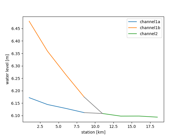
Click to see the graphTherefore, we define the following function for plotting the water level profiles gained for the simulation period’s end:
>>> def plot_waterlevels(figname):
...      import numpy
...      from matplotlib import pyplot
...      from hydpy.core.testtools import save_autofig
...      stations = ((cs := numpy.cumsum((0.0,) + lengths))[:-1] + cs[1:]) / 2.0
...      for element in (channel1a, channel1b, channel2):
...          ss = [s + sum(lengths) * (element is channel2) for s in stations]
...          ws = [sm.sequences.factors.waterlevel for sm in element.model.storagemodels]
...          _ = pyplot.plot(ss, ws, label=element.name)
...      for element in (channel1a, channel1b):
...          ss = stations[-1], stations[0] + sum(lengths)
...          ws = (element.model.storagemodels[-1].sequences.factors.waterlevel.value,
...                channel2.model.storagemodels[0].sequences.factors.waterlevel.value)
...          _ = pyplot.plot(ss, ws, color="grey")
...      _ = pyplot.legend()
...      _ = pyplot.xlabel("station [km]")
...      _ = pyplot.ylabel("water level [m]")
...      save_autofig(figname)
The simulated water levels look reasonable and are sufficiently similar to those we calculated with a fully hydrodynamic model for comparison:
>>> plot_waterlevels("sw1d_network_confluences.png")
There is no indication of an error in the water balance:
>>> round_(test.hydpy.collectives[0].model.check_waterbalance(conditions))
0.0
Bifurcations
sw1d_network also allows us to model the bifurcation of channels. We could
demonstrate this by building an entirely new setting but prefer to reuse the existing
network and just let the water flow “upstream”, which is the same in the end.
First, we break the connections to the sw1d_weir_out submodel at the outlet location
of channel2:
>>> channel2.model.storagemodels[-1].routingmodelsdownstream.number = 0
>>> channel2.model.routingmodels[-2].routingmodelsdownstream.number = 0
Second, we replace the weir model with an instance of sw1d_q_out, which is
functionally nearly identical to sw1d_q_in but to be placed at outlet locations:
>>> from hydpy.models import sw1d_q_out
>>> with channel2.model.add_routingmodel_v3(sw1d_q_out, position=4):
...     lengthupstream(2.0)
...     timestepfactor(0.7)
...     with model.add_crosssection_v2("wq_trapeze"):
...         nmbtrapezes(1)
...         bottomlevels(5.0)
...         bottomwidths(5.0)
...         sideslopes(0.0)
>>> channel2.model.connect()
We set the initial conditions as in the Confluences example:
>>> test = IntegrationTest()
>>> prepare_inits(channel1a=1.0, channel1b=1.0, channel2=1.0)
We let the same amount of water flow in the opposite direction by setting the inflow of channel1a and channel1b to zero and the outflow of channel2 to -1.5 m³/s:
>>> q_1a_in.sequences.sim.series = 0.0
>>> q_1b_in.sequences.sim.series = 0.0
>>> q_2_out.sequences.sim.series = -1.5
The outlet node q_2_out needs further attention. Usually, outlet nodes receive data
from their entry elements, but this one is supposed to send data “upstream”, which is
possible by choosing one of the available “bidirectional” deploy modes. We select
oldsim_bi (the documentation on deploymode explains this and the further
options in more detail):
>>> q_2_out.deploymode = "oldsim_bi"
Considering the absolute amount, the discharge simulated at the central node q_1to2 is quite similar to the one of the Confluences example:
>>> conditions = test("sw1d_network_branch", get_conditions="2000-01-01 00:00")
Click to see the table
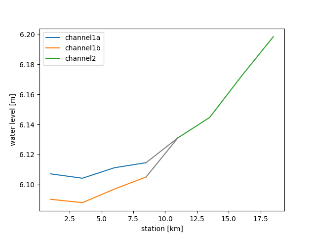
Click to see the graphAgain, the simulated water levels at the end of the simulation period seem reasonable and sufficiently similar to those we calculated with a fully hydrodynamic model:
>>> plot_waterlevels("sw1d_network_bifurcations.png")
There is no indication of an error in the water balance:
>>> round_(test.hydpy.collectives[0].model.check_waterbalance(conditions))
0.0
- class hydpy.models.sw1d_network.Model[source]
Bases:
SubstepModelHydPy-SW1D-Network (“composite model” for solving the 1-dimensional shallow water equations in channel networks).
- The following “run methods” are called in the given sequence during each simulation step:
Calc_MaxTimeSteps_V1Order all submodels that follow theRoutingModel_V1,RoutingModel_V2, orRoutingModel_V3interface to estimate the highest possible computation time step.Calc_TimeStep_V1Determine the computation time step for which we can expect stability for a complete channel network.Send_TimeStep_V1Send the actual computation time step to all submodels following theStorageModel_V1,RoutingModel_V1,RoutingModel_V2, orRoutingModel_V3interface.Calc_Discharges_V1Let a network model order all routing submodels following theRoutingModel_V1,RoutingModel_V2, orRoutingModel_V3interface to determine their individual discharge values.Update_Storages_V1Let a network model order all storage submodels to update their storage contents and their dependent factors.
- Users can hook submodels into the defined main model if they satisfy one of the following interfaces:
RoutingModel_V1Interface for calculating the inflow into a channel.RoutingModel_V2Interface for calculating the discharge between two channel segments.RoutingModel_V3Interface for calculating the outflow of a channel.StorageModel_V1Interface for calculating the water amount stored in a single channel segment.ChannelModel_V1Interface for handling routing and storage submodels.
- DOCNAME = ('SW1D-Network', '"composite model" for solving the 1-dimensional shallow water equations in channel networks')
- COMPOSITE = True
sw1d_networkis a composite model. (One usually only works with it indirectly.)
- channelmodels
Vector of submodels that comply with the following interface: ChannelModel_V1.
- storagemodels
Vector of submodels that comply with the following interface: StorageModel_V1.
- routingmodels
Vector of submodels that comply with the following interfaces: RoutingModel_V1, RoutingModel_V2, or RoutingModel_V3.
- check_waterbalance(initial_conditions: dict[str, dict[str, dict[str, float | NDArray[float64]]]]) float[source]
Determine the water balance error of the previous simulation in 1000 m³.
Method
check_waterbalance()calculates the balance error as follows:\[\begin{split}Error = \Sigma In - \Sigma Out + \Sigma Lat - \Delta Vol \\ \\ \Sigma In = \sum_{t=t_0}^{t_1} \sum_{i=1}^{R_1} DischargeVolume_t^i \\ \Sigma Out = \sum_{t=t_0}^{t_1} \sum_{i=1}^{R_3} DischargeVolume_t^i \\ \Sigma Lat = Seconds \cdot \sum_{t=t_0}^{t_1} \sum_{i=1}^{S_1} LateralFlow_t^i \\ \Delta Vol = 1000 \cdot \sum_{i=1}^{S_1} WaterVolume_{t_1}^i - WaterVolume_{t_0}^i \\ \\ S_1 = N(StorageModel\_V1) \\ R_1 = N(RoutingModel\_V1) \\ R_3 = N(RoutingModel\_V3)\end{split}\]The returned error should always be in scale with numerical precision so that it does not affect the simulation results in any relevant manner.
Pick the required initial conditions before starting the simulation run via property
conditions. See the application modelsw1d_networkfor integration tests some examples.- ToDo: So far,
check_waterbalance()works only safely with application models
sw1d_storage,sw1d_q_in,sw1d_lias,sw1d_lias_sluice,sw1d_q_out,sw1d_weir_out, andsw1d_gate_outand might fail for o ther models. We need to implement a more general solution when we implement incompatible models.
- ToDo: So far,
- REUSABLE_METHODS = ()
- class hydpy.models.sw1d_network.DerivedParameters(master: Parameters[TM_co], cls_fastaccess: type[FastAccessParameter] | None = None, cymodel: CyModelProtocol | None = None)
Bases:
DerivedParametersDerived parameters of model sw1d_network.
- The following classes are selected:
Seconds()The length of the actual simulation step size in seconds [s].
- class hydpy.models.sw1d_network.FactorSequences(master: Sequences[TM_co], cls_fastaccess: type[TypeFastAccess_co] | None = None, cymodel: CyModelProtocol | None = None)
Bases:
FactorSequencesFactor sequences of model sw1d_network.
- The following classes are selected:
TimeStep()The actual computation step according to global stability considerations [s].