The applied solver is an explicit Runge-Kutta method, which is unsuitable for solving
stiff initial value problems. Its adaptive order and stepsize control prevent
inaccurate results caused by stability issues. But for very responsive dams, increased
computation times are possible. For such cases, dam_v001 provides a less accurate
but more stable fallback mechanism. We come back to this point at the end of this
section.
Integration tests
We perform all of the following examples over 20 days:
>>> from hydpy import pub
>>> pub.timegrids = "01.01.2000", "21.01.2000", "1d"
The first examples demonstrate how dam_v001 reduces drought events at a cross-section
far downstream under different configurations. In real cases, this requires taking the
travel time of the released water into account. Therefore, we will use the
arma_rimorido application model to route the dam’s outflow to the cross-section under
investigation. Furthermore, we add some “natural” discharge to the cross-section,
reflecting the influence of the subcatchment between the dam and the cross-section.
We define four Node objects:
Node ‘inflow’ passes the inflow into the dam.
Node ‘natural’ handles the subcatchment’s additional discharge.
Node ‘outflow’ receives the dam’s (unmodified) outflow.
Node ‘remote’ receives the dam’s routed outflow and the subcatchment’s additional
discharge.
>>> from hydpy import Node
>>> inflow = Node("inflow")
>>> outflow = Node("outflow")
>>> natural = Node("natural")
>>> remote = Node("remote")
We use these nodes to connect the following three elements:
Element dam handles the tested dam_v001 model instance.
Element stream1 uses one arma_rimorido model instance to route the dam’s outflow
with significant delay.
Element stream2 uses another arma_rimorido model instance to pass the
subcatchment’s additional discharge without delay.
>>> from hydpy import Element
>>> dam = Element("dam", inlets=inflow, outlets=outflow, receivers=remote)
>>> stream1 = Element("stream1", inlets=outflow, outlets=remote)
>>> stream2 = Element("stream2", inlets=natural, outlets=remote)
Next, we prepare the three model instances. We begin with the stream2 model.
Setting the Responses parameter in the following manner defines a pure
Moving Average model that neither results in translation nor retention:
>>> from hydpy import prepare_model
>>> stream2.model = prepare_model("arma_rimorido")
>>> stream2.model.parameters.control.responses(((), (1.0,)))
>>> stream2.model.parameters.update()
stream2 also works like a pure Moving Average model, but causes a time delay of
1.8 days:
>>> stream1.model = prepare_model("arma_rimorido")
>>> stream1.model.parameters.control.responses(((), (0.2, 0.4, 0.3, 0.1)))
>>> stream1.model.parameters.update()
Last but not least, we initialise the dam_v001 instance and hand it to its element
(we will define distinct parameter sets for the examples below):
>>> from hydpy.models.dam_v001 import *
>>> parameterstep("1d")
>>> dam.model = model
The IntegrationTest object test serves to execute the following examples
conveniently:
>>> from hydpy import IntegrationTest
>>> test = IntegrationTest(dam)
>>> test.inits=((states.watervolume, 0.0),
...             (logs.loggedadjustedevaporation, 0.0),
...             (logs.loggedtotalremotedischarge, 1.9),
...             (logs.loggedoutflow, 0.0),
...             (stream1.model.sequences.logs.login, 0.0))
>>> test.dateformat = "%d.%m."
>>> test.plotting_options.axis1 = fluxes.inflow, fluxes.outflow
>>> test.plotting_options.axis2 = states.watervolume
Next, we create a drought event. The natural discharge of the subcatchment decreases
for nine days, stays at a constant level of 1 m³/s for four days, and increases again:
>>> natural.sequences.sim.series = [1.8, 1.7, 1.6, 1.5, 1.4, 1.3, 1.2, 1.1, 1.0, 1.0,
...                                 1.0, 1.0, 1.1, 1.2, 1.3, 1.4, 1.5, 1.6, 1.7, 1.8]
The inflow into the dam remains constant for the whole simulation period:
>>> inflow.sequences.sim.series = 1.0
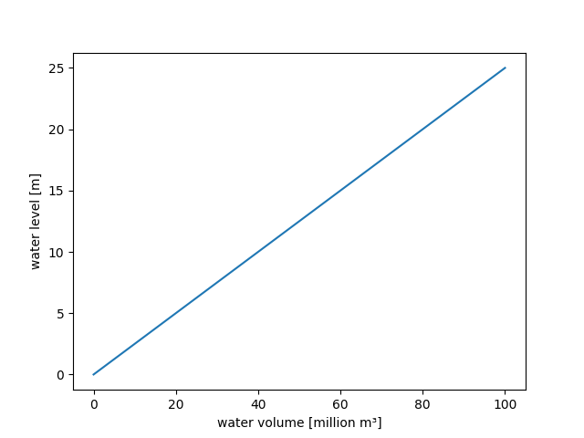
For the sake of simplicity, we define a linear relationship between the stored water
volume and the water level. One can accomplish this most easily via method
from_data() of class PPoly:
>>> watervolume2waterlevel(PPoly.from_data(xs=[0.0, 1.0], ys=[0.0, 0.25]))
The following figure confirms the linearity of the defined relationship:
>>> figure = watervolume2waterlevel.plot(0.0, 100.0)
>>> from hydpy.core.testtools import save_autofig
>>> save_autofig("dam_v001_watervolume2waterlevel.png", figure=figure)
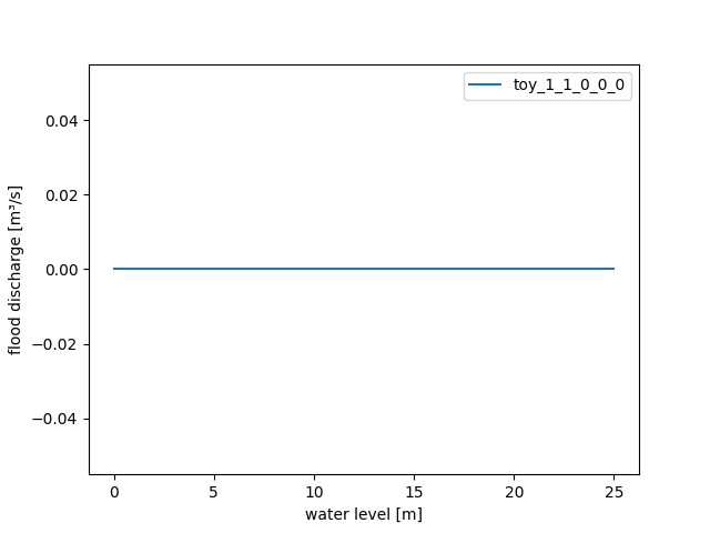
To focus on the drought-related algorithms only, we turn off the flood-related
processes. Therefore, we let parameter WaterLevel2FloodDischarge return zero for all
possible input values:
>>> waterlevel2flooddischarge(PPoly.from_data(xs=[0.0], ys=[0.0]))
>>> figure = waterlevel2flooddischarge.plot(0.0, 25.0)
>>> save_autofig("dam_v001_waterlevel2flooddischarge_1.png", figure=figure)
The exact values of the following parameters are relevant only for those examples where
we take precipitation or evaporation into account. Please see the documentation on the
simple lake model dam_llake, which discusses these parameters in detail:
>>> surfacearea(1.44)
>>> correctionprecipitation(1.2)
>>> correctionevaporation(1.2)
>>> weightevaporation(0.8)
>>> thresholdevaporation(0.0)
>>> toleranceevaporation(0.001)
We must define the catchment area draining into the dam. dam_v001 requires this
information to adjust the numerical local truncation error. For a catchment area of
86.4 km², the general local truncation error (in mm per simulation step) is identical
to the applied site-specific local truncation error (in m³/s):
>>> catchmentarea(86.4)
>>> from hydpy import round_
>>> round_(solver.abserrormax.INIT)
0.0001
>>> derived.seconds.update()
>>> solver.abserrormax.update()
>>> solver.abserrormax
abserrormax(0.0001)
If you require higher accuracy or can live with lower accuracy, override this default
mechanism by setting any other tolerance value (possible within any control file; see
the accuracy drought and the accuracy flood examples
for further information).
We enable the RestrictTargetedRelease option flag in the following examples unless
stated otherwise:
>>> restricttargetedrelease(True)
no outflow
We temporarily turn off the drought-related functionalities to confirm the proper
arrangement of the whole scenario.
>>> nmblogentries(1)
>>> remotedischargeminimum(0.0)
>>> remotedischargesafety(0.0)
>>> neardischargeminimumthreshold(0.0)
>>> neardischargeminimumtolerance(0.0)
>>> waterlevelminimumthreshold(0.0)
>>> waterlevelminimumtolerance(0.0)
The following table confirms that dam_v001 does not release any discharge (the column
“outflow” contains zero values only). Hence, the downstream cross-section’s discharge
(column “remote”) and the subcatchment’s discharge (column “natural”) are identical:
>>> test("dam_v001_no_outflow")
Click to see the table
| date | waterlevel | precipitation | adjustedprecipitation | potentialevaporation | adjustedevaporation | actualevaporation | inflow | totalremotedischarge | naturalremotedischarge | remotedemand | remotefailure | requiredremoterelease | requiredrelease | targetedrelease | actualrelease | flooddischarge | outflow | watervolume | inflow | natural | outflow | remote |
-----------------------------------------------------------------------------------------------------------------------------------------------------------------------------------------------------------------------------------------------------------------------------------------------------------------------------------------------------------------------------------
| 01.01. | 0.0216 | 0.0 | 0.0 | 0.0 | 0.0 | 0.0 | 1.0 | 1.8 | 1.9 | 0.0 | -1.9 | 0.0 | 0.0 | 0.0 | 0.0 | 0.0 | 0.0 | 0.0864 | 1.0 | 1.8 | 0.0 | 1.8 |
| 02.01. | 0.0432 | 0.0 | 0.0 | 0.0 | 0.0 | 0.0 | 1.0 | 1.7 | 1.8 | 0.0 | -1.8 | 0.0 | 0.0 | 0.0 | 0.0 | 0.0 | 0.0 | 0.1728 | 1.0 | 1.7 | 0.0 | 1.7 |
| 03.01. | 0.0648 | 0.0 | 0.0 | 0.0 | 0.0 | 0.0 | 1.0 | 1.6 | 1.7 | 0.0 | -1.7 | 0.0 | 0.0 | 0.0 | 0.0 | 0.0 | 0.0 | 0.2592 | 1.0 | 1.6 | 0.0 | 1.6 |
| 04.01. | 0.0864 | 0.0 | 0.0 | 0.0 | 0.0 | 0.0 | 1.0 | 1.5 | 1.6 | 0.0 | -1.6 | 0.0 | 0.0 | 0.0 | 0.0 | 0.0 | 0.0 | 0.3456 | 1.0 | 1.5 | 0.0 | 1.5 |
| 05.01. | 0.108 | 0.0 | 0.0 | 0.0 | 0.0 | 0.0 | 1.0 | 1.4 | 1.5 | 0.0 | -1.5 | 0.0 | 0.0 | 0.0 | 0.0 | 0.0 | 0.0 | 0.432 | 1.0 | 1.4 | 0.0 | 1.4 |
| 06.01. | 0.1296 | 0.0 | 0.0 | 0.0 | 0.0 | 0.0 | 1.0 | 1.3 | 1.4 | 0.0 | -1.4 | 0.0 | 0.0 | 0.0 | 0.0 | 0.0 | 0.0 | 0.5184 | 1.0 | 1.3 | 0.0 | 1.3 |
| 07.01. | 0.1512 | 0.0 | 0.0 | 0.0 | 0.0 | 0.0 | 1.0 | 1.2 | 1.3 | 0.0 | -1.3 | 0.0 | 0.0 | 0.0 | 0.0 | 0.0 | 0.0 | 0.6048 | 1.0 | 1.2 | 0.0 | 1.2 |
| 08.01. | 0.1728 | 0.0 | 0.0 | 0.0 | 0.0 | 0.0 | 1.0 | 1.1 | 1.2 | 0.0 | -1.2 | 0.0 | 0.0 | 0.0 | 0.0 | 0.0 | 0.0 | 0.6912 | 1.0 | 1.1 | 0.0 | 1.1 |
| 09.01. | 0.1944 | 0.0 | 0.0 | 0.0 | 0.0 | 0.0 | 1.0 | 1.0 | 1.1 | 0.0 | -1.1 | 0.0 | 0.0 | 0.0 | 0.0 | 0.0 | 0.0 | 0.7776 | 1.0 | 1.0 | 0.0 | 1.0 |
| 10.01. | 0.216 | 0.0 | 0.0 | 0.0 | 0.0 | 0.0 | 1.0 | 1.0 | 1.0 | 0.0 | -1.0 | 0.0 | 0.0 | 0.0 | 0.0 | 0.0 | 0.0 | 0.864 | 1.0 | 1.0 | 0.0 | 1.0 |
| 11.01. | 0.2376 | 0.0 | 0.0 | 0.0 | 0.0 | 0.0 | 1.0 | 1.0 | 1.0 | 0.0 | -1.0 | 0.0 | 0.0 | 0.0 | 0.0 | 0.0 | 0.0 | 0.9504 | 1.0 | 1.0 | 0.0 | 1.0 |
| 12.01. | 0.2592 | 0.0 | 0.0 | 0.0 | 0.0 | 0.0 | 1.0 | 1.0 | 1.0 | 0.0 | -1.0 | 0.0 | 0.0 | 0.0 | 0.0 | 0.0 | 0.0 | 1.0368 | 1.0 | 1.0 | 0.0 | 1.0 |
| 13.01. | 0.2808 | 0.0 | 0.0 | 0.0 | 0.0 | 0.0 | 1.0 | 1.1 | 1.0 | 0.0 | -1.0 | 0.0 | 0.0 | 0.0 | 0.0 | 0.0 | 0.0 | 1.1232 | 1.0 | 1.1 | 0.0 | 1.1 |
| 14.01. | 0.3024 | 0.0 | 0.0 | 0.0 | 0.0 | 0.0 | 1.0 | 1.2 | 1.1 | 0.0 | -1.1 | 0.0 | 0.0 | 0.0 | 0.0 | 0.0 | 0.0 | 1.2096 | 1.0 | 1.2 | 0.0 | 1.2 |
| 15.01. | 0.324 | 0.0 | 0.0 | 0.0 | 0.0 | 0.0 | 1.0 | 1.3 | 1.2 | 0.0 | -1.2 | 0.0 | 0.0 | 0.0 | 0.0 | 0.0 | 0.0 | 1.296 | 1.0 | 1.3 | 0.0 | 1.3 |
| 16.01. | 0.3456 | 0.0 | 0.0 | 0.0 | 0.0 | 0.0 | 1.0 | 1.4 | 1.3 | 0.0 | -1.3 | 0.0 | 0.0 | 0.0 | 0.0 | 0.0 | 0.0 | 1.3824 | 1.0 | 1.4 | 0.0 | 1.4 |
| 17.01. | 0.3672 | 0.0 | 0.0 | 0.0 | 0.0 | 0.0 | 1.0 | 1.5 | 1.4 | 0.0 | -1.4 | 0.0 | 0.0 | 0.0 | 0.0 | 0.0 | 0.0 | 1.4688 | 1.0 | 1.5 | 0.0 | 1.5 |
| 18.01. | 0.3888 | 0.0 | 0.0 | 0.0 | 0.0 | 0.0 | 1.0 | 1.6 | 1.5 | 0.0 | -1.5 | 0.0 | 0.0 | 0.0 | 0.0 | 0.0 | 0.0 | 1.5552 | 1.0 | 1.6 | 0.0 | 1.6 |
| 19.01. | 0.4104 | 0.0 | 0.0 | 0.0 | 0.0 | 0.0 | 1.0 | 1.7 | 1.6 | 0.0 | -1.6 | 0.0 | 0.0 | 0.0 | 0.0 | 0.0 | 0.0 | 1.6416 | 1.0 | 1.7 | 0.0 | 1.7 |
| 20.01. | 0.432 | 0.0 | 0.0 | 0.0 | 0.0 | 0.0 | 1.0 | 1.8 | 1.7 | 0.0 | -1.7 | 0.0 | 0.0 | 0.0 | 0.0 | 0.0 | 0.0 | 1.728 | 1.0 | 1.8 | 0.0 | 1.8 |
exact remote minimum
Now, we set the discharge to be not undercut at the cross-section downstream to
1.4 m³/s:
>>> remotedischargeminimum(1.4)
Principally, the dam model attenuates the drought. However, it is not very successful
in doing so. In the event’s first half, the cross-section’s lowest discharge increases
from 1.0 m³/s to approximately 1.2 m³/s, which is still below the threshold value of
1.4 m³/s. Furthermore, in the event’s second half, dam_v001 works too eagerly,
resulting in a discharge of approximately 1.6 m³/s instead of 1.4 m³/s on January 12:
>>> test("dam_v001_exact_remote_minimum")
Click to see the table
| date | waterlevel | precipitation | adjustedprecipitation | potentialevaporation | adjustedevaporation | actualevaporation | inflow | totalremotedischarge | naturalremotedischarge | remotedemand | remotefailure | requiredremoterelease | requiredrelease | targetedrelease | actualrelease | flooddischarge | outflow | watervolume | inflow | natural | outflow | remote |
---------------------------------------------------------------------------------------------------------------------------------------------------------------------------------------------------------------------------------------------------------------------------------------------------------------------------------------------------------------------------------------
| 01.01. | 0.0216 | 0.0 | 0.0 | 0.0 | 0.0 | 0.0 | 1.0 | 1.8 | 1.9 | 0.0 | -0.5 | 0.0 | 0.0 | 0.0 | 0.0 | 0.0 | 0.0 | 0.0864 | 1.0 | 1.8 | 0.0 | 1.8 |
| 02.01. | 0.0432 | 0.0 | 0.0 | 0.0 | 0.0 | 0.0 | 1.0 | 1.7 | 1.8 | 0.0 | -0.4 | 0.0 | 0.0 | 0.0 | 0.0 | 0.0 | 0.0 | 0.1728 | 1.0 | 1.7 | 0.0 | 1.7 |
| 03.01. | 0.0648 | 0.0 | 0.0 | 0.0 | 0.0 | 0.0 | 1.0 | 1.6 | 1.7 | 0.0 | -0.3 | 0.0 | 0.0 | 0.0 | 0.0 | 0.0 | 0.0 | 0.2592 | 1.0 | 1.6 | 0.0 | 1.6 |
| 04.01. | 0.0864 | 0.0 | 0.0 | 0.0 | 0.0 | 0.0 | 1.0 | 1.5 | 1.6 | 0.0 | -0.2 | 0.0 | 0.0 | 0.0 | 0.0 | 0.0 | 0.0 | 0.3456 | 1.0 | 1.5 | 0.0 | 1.5 |
| 05.01. | 0.108 | 0.0 | 0.0 | 0.0 | 0.0 | 0.0 | 1.0 | 1.4 | 1.5 | 0.0 | -0.1 | 0.0 | 0.0 | 0.0 | 0.0 | 0.0 | 0.0 | 0.432 | 1.0 | 1.4 | 0.0 | 1.4 |
| 06.01. | 0.1296 | 0.0 | 0.0 | 0.0 | 0.0 | 0.0 | 1.0 | 1.3 | 1.4 | 0.0 | 0.0 | 0.0 | 0.0 | 0.0 | 0.0 | 0.0 | 0.0 | 0.5184 | 1.0 | 1.3 | 0.0 | 1.3 |
| 07.01. | 0.14904 | 0.0 | 0.0 | 0.0 | 0.0 | 0.0 | 1.0 | 1.22 | 1.3 | 0.1 | 0.1 | 0.1 | 0.1 | 0.1 | 0.1 | 0.0 | 0.1 | 0.59616 | 1.0 | 1.2 | 0.1 | 1.22 |
| 08.01. | 0.164592 | 0.0 | 0.0 | 0.0 | 0.0 | 0.0 | 1.0 | 1.196 | 1.12 | 0.28 | 0.18 | 0.28 | 0.28 | 0.28 | 0.28 | 0.0 | 0.28 | 0.658368 | 1.0 | 1.1 | 0.28 | 1.196 |
| 09.01. | 0.175738 | 0.0 | 0.0 | 0.0 | 0.0 | 0.0 | 1.0 | 1.2388 | 0.916 | 0.484 | 0.204 | 0.484 | 0.484 | 0.484 | 0.484 | 0.0 | 0.484 | 0.70295 | 1.0 | 1.0 | 0.484 | 1.2388 |
| 10.01. | 0.183401 | 0.0 | 0.0 | 0.0 | 0.0 | 0.0 | 1.0 | 1.41664 | 0.7548 | 0.6452 | 0.1612 | 0.6452 | 0.6452 | 0.6452 | 0.6452 | 0.0 | 0.6452 | 0.733605 | 1.0 | 1.0 | 0.6452 | 1.41664 |
| 11.01. | 0.191424 | 0.0 | 0.0 | 0.0 | 0.0 | 0.0 | 1.0 | 1.556992 | 0.77144 | 0.62856 | -0.01664 | 0.62856 | 0.62856 | 0.62856 | 0.62856 | 0.0 | 0.62856 | 0.765698 | 1.0 | 1.0 | 0.62856 | 1.556992 |
| 12.01. | 0.202839 | 0.0 | 0.0 | 0.0 | 0.0 | 0.0 | 1.0 | 1.587698 | 0.928432 | 0.471568 | -0.156992 | 0.471568 | 0.471568 | 0.471568 | 0.471568 | 0.0 | 0.471568 | 0.811354 | 1.0 | 1.0 | 0.471568 | 1.587698 |
| 13.01. | 0.218307 | 0.0 | 0.0 | 0.0 | 0.0 | 0.0 | 1.0 | 1.598489 | 1.11613 | 0.28387 | -0.187698 | 0.28387 | 0.28387 | 0.28387 | 0.28387 | 0.0 | 0.28387 | 0.873228 | 1.0 | 1.1 | 0.28387 | 1.598489 |
| 14.01. | 0.238063 | 0.0 | 0.0 | 0.0 | 0.0 | 0.0 | 1.0 | 1.534951 | 1.314619 | 0.085381 | -0.198489 | 0.085381 | 0.085381 | 0.085381 | 0.085381 | 0.0 | 0.085381 | 0.952251 | 1.0 | 1.2 | 0.085381 | 1.534951 |
| 15.01. | 0.259663 | 0.0 | 0.0 | 0.0 | 0.0 | 0.0 | 1.0 | 1.46647 | 1.44957 | 0.0 | -0.134951 | 0.0 | 0.0 | 0.0 | 0.0 | 0.0 | 0.0 | 1.038651 | 1.0 | 1.3 | 0.0 | 1.46647 |
| 16.01. | 0.281263 | 0.0 | 0.0 | 0.0 | 0.0 | 0.0 | 1.0 | 1.454001 | 1.46647 | 0.0 | -0.06647 | 0.0 | 0.0 | 0.0 | 0.0 | 0.0 | 0.0 | 1.125051 | 1.0 | 1.4 | 0.0 | 1.454001 |
| 17.01. | 0.302863 | 0.0 | 0.0 | 0.0 | 0.0 | 0.0 | 1.0 | 1.508538 | 1.454001 | 0.0 | -0.054001 | 0.0 | 0.0 | 0.0 | 0.0 | 0.0 | 0.0 | 1.211451 | 1.0 | 1.5 | 0.0 | 1.508538 |
| 18.01. | 0.324463 | 0.0 | 0.0 | 0.0 | 0.0 | 0.0 | 1.0 | 1.6 | 1.508538 | 0.0 | -0.108538 | 0.0 | 0.0 | 0.0 | 0.0 | 0.0 | 0.0 | 1.297851 | 1.0 | 1.6 | 0.0 | 1.6 |
| 19.01. | 0.346063 | 0.0 | 0.0 | 0.0 | 0.0 | 0.0 | 1.0 | 1.7 | 1.6 | 0.0 | -0.2 | 0.0 | 0.0 | 0.0 | 0.0 | 0.0 | 0.0 | 1.384251 | 1.0 | 1.7 | 0.0 | 1.7 |
| 20.01. | 0.367663 | 0.0 | 0.0 | 0.0 | 0.0 | 0.0 | 1.0 | 1.8 | 1.7 | 0.0 | -0.3 | 0.0 | 0.0 | 0.0 | 0.0 | 0.0 | 0.0 | 1.470651 | 1.0 | 1.8 | 0.0 | 1.8 |
increased remote minimum
The qualified success in the example above is partly due to the time delay of the
information flow from the cross-section to the dam, but the more important factor is
the travel time of the released discharge. A simple strategy to increase reliability
is to set a higher value for parameter RemoteDischargeMinimum. When defining a value
of 1.6 m/s, only minor violations of the actual threshold value remain:
>>> remotedischargeminimum(1.6)
>>> test("dam_v001_increased_remote_minimum")
Click to see the table
| date | waterlevel | precipitation | adjustedprecipitation | potentialevaporation | adjustedevaporation | actualevaporation | inflow | totalremotedischarge | naturalremotedischarge | remotedemand | remotefailure | requiredremoterelease | requiredrelease | targetedrelease | actualrelease | flooddischarge | outflow | watervolume | inflow | natural | outflow | remote |
---------------------------------------------------------------------------------------------------------------------------------------------------------------------------------------------------------------------------------------------------------------------------------------------------------------------------------------------------------------------------------------
| 01.01. | 0.0216 | 0.0 | 0.0 | 0.0 | 0.0 | 0.0 | 1.0 | 1.8 | 1.9 | 0.0 | -0.3 | 0.0 | 0.0 | 0.0 | 0.0 | 0.0 | 0.0 | 0.0864 | 1.0 | 1.8 | 0.0 | 1.8 |
| 02.01. | 0.0432 | 0.0 | 0.0 | 0.0 | 0.0 | 0.0 | 1.0 | 1.7 | 1.8 | 0.0 | -0.2 | 0.0 | 0.0 | 0.0 | 0.0 | 0.0 | 0.0 | 0.1728 | 1.0 | 1.7 | 0.0 | 1.7 |
| 03.01. | 0.0648 | 0.0 | 0.0 | 0.0 | 0.0 | 0.0 | 1.0 | 1.6 | 1.7 | 0.0 | -0.1 | 0.0 | 0.0 | 0.0 | 0.0 | 0.0 | 0.0 | 0.2592 | 1.0 | 1.6 | 0.0 | 1.6 |
| 04.01. | 0.0864 | 0.0 | 0.0 | 0.0 | 0.0 | 0.0 | 1.0 | 1.5 | 1.6 | 0.0 | 0.0 | 0.0 | 0.0 | 0.0 | 0.0 | 0.0 | 0.0 | 0.3456 | 1.0 | 1.5 | 0.0 | 1.5 |
| 05.01. | 0.10584 | 0.0 | 0.0 | 0.0 | 0.0 | 0.0 | 1.0 | 1.42 | 1.5 | 0.1 | 0.1 | 0.1 | 0.1 | 0.1 | 0.1 | 0.0 | 0.1 | 0.42336 | 1.0 | 1.4 | 0.1 | 1.42 |
| 06.01. | 0.121392 | 0.0 | 0.0 | 0.0 | 0.0 | 0.0 | 1.0 | 1.396 | 1.32 | 0.28 | 0.18 | 0.28 | 0.28 | 0.28 | 0.28 | 0.0 | 0.28 | 0.485568 | 1.0 | 1.3 | 0.28 | 1.396 |
| 07.01. | 0.132538 | 0.0 | 0.0 | 0.0 | 0.0 | 0.0 | 1.0 | 1.4388 | 1.116 | 0.484 | 0.204 | 0.484 | 0.484 | 0.484 | 0.484 | 0.0 | 0.484 | 0.53015 | 1.0 | 1.2 | 0.484 | 1.4388 |
| 08.01. | 0.140201 | 0.0 | 0.0 | 0.0 | 0.0 | 0.0 | 1.0 | 1.51664 | 0.9548 | 0.6452 | 0.1612 | 0.6452 | 0.6452 | 0.6452 | 0.6452 | 0.0 | 0.6452 | 0.560805 | 1.0 | 1.1 | 0.6452 | 1.51664 |
| 09.01. | 0.146064 | 0.0 | 0.0 | 0.0 | 0.0 | 0.0 | 1.0 | 1.576992 | 0.87144 | 0.72856 | 0.08336 | 0.72856 | 0.72856 | 0.72856 | 0.72856 | 0.0 | 0.72856 | 0.584258 | 1.0 | 1.0 | 0.72856 | 1.576992 |
| 10.01. | 0.151431 | 0.0 | 0.0 | 0.0 | 0.0 | 0.0 | 1.0 | 1.683698 | 0.848432 | 0.751568 | 0.023008 | 0.751568 | 0.751568 | 0.751568 | 0.751568 | 0.0 | 0.751568 | 0.605722 | 1.0 | 1.0 | 0.751568 | 1.683698 |
| 11.01. | 0.158605 | 0.0 | 0.0 | 0.0 | 0.0 | 0.0 | 1.0 | 1.717289 | 0.93213 | 0.66787 | -0.083698 | 0.66787 | 0.66787 | 0.66787 | 0.66787 | 0.0 | 0.66787 | 0.634418 | 1.0 | 1.0 | 0.66787 | 1.717289 |
| 12.01. | 0.168312 | 0.0 | 0.0 | 0.0 | 0.0 | 0.0 | 1.0 | 1.675591 | 1.049419 | 0.550581 | -0.117289 | 0.550581 | 0.550581 | 0.550581 | 0.550581 | 0.0 | 0.550581 | 0.673248 | 1.0 | 1.0 | 0.550581 | 1.675591 |
| 13.01. | 0.179652 | 0.0 | 0.0 | 0.0 | 0.0 | 0.0 | 1.0 | 1.690748 | 1.12501 | 0.47499 | -0.075591 | 0.47499 | 0.47499 | 0.47499 | 0.47499 | 0.0 | 0.47499 | 0.718609 | 1.0 | 1.1 | 0.47499 | 1.690748 |
| 14.01. | 0.192953 | 0.0 | 0.0 | 0.0 | 0.0 | 0.0 | 1.0 | 1.698806 | 1.215758 | 0.384242 | -0.090748 | 0.384242 | 0.384242 | 0.384242 | 0.384242 | 0.0 | 0.384242 | 0.77181 | 1.0 | 1.2 | 0.384242 | 1.698806 |
| 15.01. | 0.208387 | 0.0 | 0.0 | 0.0 | 0.0 | 0.0 | 1.0 | 1.708339 | 1.314564 | 0.285436 | -0.098806 | 0.285436 | 0.285436 | 0.285436 | 0.285436 | 0.0 | 0.285436 | 0.833549 | 1.0 | 1.3 | 0.285436 | 1.708339 |
| 16.01. | 0.226162 | 0.0 | 0.0 | 0.0 | 0.0 | 0.0 | 1.0 | 1.712365 | 1.422903 | 0.177097 | -0.108339 | 0.177097 | 0.177097 | 0.177097 | 0.177097 | 0.0 | 0.177097 | 0.904647 | 1.0 | 1.4 | 0.177097 | 1.712365 |
| 17.01. | 0.246364 | 0.0 | 0.0 | 0.0 | 0.0 | 0.0 | 1.0 | 1.70784 | 1.535269 | 0.064731 | -0.112365 | 0.064731 | 0.064731 | 0.064731 | 0.064731 | 0.0 | 0.064731 | 0.985455 | 1.0 | 1.5 | 0.064731 | 1.70784 |
| 18.01. | 0.267964 | 0.0 | 0.0 | 0.0 | 0.0 | 0.0 | 1.0 | 1.707565 | 1.643109 | 0.0 | -0.10784 | 0.0 | 0.0 | 0.0 | 0.0 | 0.0 | 0.0 | 1.071855 | 1.0 | 1.6 | 0.0 | 1.707565 |
| 19.01. | 0.289564 | 0.0 | 0.0 | 0.0 | 0.0 | 0.0 | 1.0 | 1.737129 | 1.707565 | 0.0 | -0.107565 | 0.0 | 0.0 | 0.0 | 0.0 | 0.0 | 0.0 | 1.158255 | 1.0 | 1.7 | 0.0 | 1.737129 |
| 20.01. | 0.311164 | 0.0 | 0.0 | 0.0 | 0.0 | 0.0 | 1.0 | 1.806473 | 1.737129 | 0.0 | -0.137129 | 0.0 | 0.0 | 0.0 | 0.0 | 0.0 | 0.0 | 1.244655 | 1.0 | 1.8 | 0.0 | 1.806473 |
remote safety
While increasing parameter RemoteDischargeMinimum is always possible, it is often
advisable to modify parameter RemoteDischargeSafety instead:
>>> remotedischargeminimum(1.4)
>>> remotedischargesafety(0.5)
For the new configuration, the cross-section’s discharge exceeds the threshold value at
each simulation time step. Additionally, the dam’s final storage content is about 4 %
higher than in the last example, indicating more efficient water usage:
>>> test("dam_v001_remote_safety")
Click to see the table
| date | waterlevel | precipitation | adjustedprecipitation | potentialevaporation | adjustedevaporation | actualevaporation | inflow | totalremotedischarge | naturalremotedischarge | remotedemand | remotefailure | requiredremoterelease | requiredrelease | targetedrelease | actualrelease | flooddischarge | outflow | watervolume | inflow | natural | outflow | remote |
---------------------------------------------------------------------------------------------------------------------------------------------------------------------------------------------------------------------------------------------------------------------------------------------------------------------------------------------------------------------------------------
| 01.01. | 0.021495 | 0.0 | 0.0 | 0.0 | 0.0 | 0.0 | 1.0 | 1.800975 | 1.9 | 0.0 | -0.5 | 0.005 | 0.005 | 0.005 | 0.004875 | 0.0 | 0.004875 | 0.085979 | 1.0 | 1.8 | 0.004875 | 1.800975 |
| 02.01. | 0.04283 | 0.0 | 0.0 | 0.0 | 0.0 | 0.0 | 1.0 | 1.704398 | 1.7961 | 0.0 | -0.400975 | 0.012241 | 0.012241 | 0.012241 | 0.012241 | 0.0 | 0.012241 | 0.171321 | 1.0 | 1.7 | 0.012241 | 1.704398 |
| 03.01. | 0.06381 | 0.0 | 0.0 | 0.0 | 0.0 | 0.0 | 1.0 | 1.612105 | 1.692157 | 0.0 | -0.304398 | 0.02873 | 0.02873 | 0.02873 | 0.02873 | 0.0 | 0.02873 | 0.255239 | 1.0 | 1.6 | 0.02873 | 1.612105 |
| 04.01. | 0.084064 | 0.0 | 0.0 | 0.0 | 0.0 | 0.0 | 1.0 | 1.528115 | 1.583375 | 0.0 | -0.212105 | 0.062315 | 0.062315 | 0.062315 | 0.062315 | 0.0 | 0.062315 | 0.336255 | 1.0 | 1.5 | 0.062315 | 1.528115 |
| 05.01. | 0.10312 | 0.0 | 0.0 | 0.0 | 0.0 | 0.0 | 1.0 | 1.458321 | 1.4658 | 0.0 | -0.128115 | 0.11776 | 0.11776 | 0.11776 | 0.11776 | 0.0 | 0.11776 | 0.41248 | 1.0 | 1.4 | 0.11776 | 1.458321 |
| 06.01. | 0.11945 | 0.0 | 0.0 | 0.0 | 0.0 | 0.0 | 1.0 | 1.417471 | 1.340561 | 0.059439 | -0.058321 | 0.244 | 0.244 | 0.244 | 0.244 | 0.0 | 0.244 | 0.477799 | 1.0 | 1.3 | 0.244 | 1.417471 |
| 07.01. | 0.131189 | 0.0 | 0.0 | 0.0 | 0.0 | 0.0 | 1.0 | 1.430459 | 1.173472 | 0.226528 | -0.017471 | 0.456501 | 0.456501 | 0.456501 | 0.456501 | 0.0 | 0.456501 | 0.524757 | 1.0 | 1.2 | 0.456501 | 1.430459 |
| 08.01. | 0.138938 | 0.0 | 0.0 | 0.0 | 0.0 | 0.0 | 1.0 | 1.495831 | 0.973959 | 0.426041 | -0.030459 | 0.641277 | 0.641277 | 0.641277 | 0.641277 | 0.0 | 0.641277 | 0.555751 | 1.0 | 1.1 | 0.641277 | 1.495831 |
| 09.01. | 0.145591 | 0.0 | 0.0 | 0.0 | 0.0 | 0.0 | 1.0 | 1.556253 | 0.854555 | 0.545445 | -0.095831 | 0.69196 | 0.69196 | 0.69196 | 0.69196 | 0.0 | 0.69196 | 0.582366 | 1.0 | 1.0 | 0.69196 | 1.556253 |
| 10.01. | 0.153545 | 0.0 | 0.0 | 0.0 | 0.0 | 0.0 | 1.0 | 1.641175 | 0.864293 | 0.535707 | -0.156253 | 0.63179 | 0.63179 | 0.63179 | 0.63179 | 0.0 | 0.63179 | 0.614179 | 1.0 | 1.0 | 0.63179 | 1.641175 |
| 11.01. | 0.165646 | 0.0 | 0.0 | 0.0 | 0.0 | 0.0 | 1.0 | 1.612383 | 1.009385 | 0.390615 | -0.241175 | 0.439756 | 0.439756 | 0.439756 | 0.439756 | 0.0 | 0.439756 | 0.662584 | 1.0 | 1.0 | 0.439756 | 1.612383 |
| 12.01. | 0.180992 | 0.0 | 0.0 | 0.0 | 0.0 | 0.0 | 1.0 | 1.492545 | 1.172627 | 0.227373 | -0.212383 | 0.289549 | 0.289549 | 0.289549 | 0.289549 | 0.0 | 0.289549 | 0.723967 | 1.0 | 1.0 | 0.289549 | 1.492545 |
| 13.01. | 0.195104 | 0.0 | 0.0 | 0.0 | 0.0 | 0.0 | 1.0 | 1.480259 | 1.202996 | 0.197004 | -0.092545 | 0.346666 | 0.346666 | 0.346666 | 0.346666 | 0.0 | 0.346666 | 0.780415 | 1.0 | 1.1 | 0.346666 | 1.480259 |
| 14.01. | 0.207455 | 0.0 | 0.0 | 0.0 | 0.0 | 0.0 | 1.0 | 1.555141 | 1.133592 | 0.266408 | -0.080259 | 0.428173 | 0.428173 | 0.428173 | 0.428173 | 0.0 | 0.428173 | 0.829821 | 1.0 | 1.2 | 0.428173 | 1.555141 |
| 15.01. | 0.221065 | 0.0 | 0.0 | 0.0 | 0.0 | 0.0 | 1.0 | 1.678206 | 1.126968 | 0.273032 | -0.155141 | 0.36991 | 0.36991 | 0.36991 | 0.36991 | 0.0 | 0.36991 | 0.884261 | 1.0 | 1.3 | 0.36991 | 1.678206 |
| 16.01. | 0.239907 | 0.0 | 0.0 | 0.0 | 0.0 | 0.0 | 1.0 | 1.73662 | 1.308296 | 0.091704 | -0.278206 | 0.12769 | 0.12769 | 0.12769 | 0.12769 | 0.0 | 0.12769 | 0.959628 | 1.0 | 1.4 | 0.12769 | 1.73662 |
| 17.01. | 0.261039 | 0.0 | 0.0 | 0.0 | 0.0 | 0.0 | 1.0 | 1.709203 | 1.608931 | 0.0 | -0.33662 | 0.021686 | 0.021686 | 0.021686 | 0.021686 | 0.0 | 0.021686 | 1.044155 | 1.0 | 1.5 | 0.021686 | 1.709203 |
| 18.01. | 0.282043 | 0.0 | 0.0 | 0.0 | 0.0 | 0.0 | 1.0 | 1.689484 | 1.687518 | 0.0 | -0.309203 | 0.027557 | 0.027557 | 0.027557 | 0.027557 | 0.0 | 0.027557 | 1.128174 | 1.0 | 1.6 | 0.027557 | 1.689484 |
| 19.01. | 0.302938 | 0.0 | 0.0 | 0.0 | 0.0 | 0.0 | 1.0 | 1.736832 | 1.661926 | 0.0 | -0.289484 | 0.032675 | 0.032675 | 0.032675 | 0.032675 | 0.0 | 0.032675 | 1.211751 | 1.0 | 1.7 | 0.032675 | 1.736832 |
| 20.01. | 0.32407 | 0.0 | 0.0 | 0.0 | 0.0 | 0.0 | 1.0 | 1.827835 | 1.704158 | 0.0 | -0.336832 | 0.021645 | 0.021645 | 0.021645 | 0.021645 | 0.0 | 0.021645 | 1.29628 | 1.0 | 1.8 | 0.021645 | 1.827835 |
sharp near minimum
Building upon the last example, we subsequently increase the model’s complexity. Next,
we introduce a local minimum water release of 0.2 m³/s:
>>> neardischargeminimumthreshold(0.2)
Consequently, dam_v001 now releases the discharge that is not required at the
cross-section downstream:
>>> test("dam_v001_sharp_near_minimum")
Click to see the table
| date | waterlevel | precipitation | adjustedprecipitation | potentialevaporation | adjustedevaporation | actualevaporation | inflow | totalremotedischarge | naturalremotedischarge | remotedemand | remotefailure | requiredremoterelease | requiredrelease | targetedrelease | actualrelease | flooddischarge | outflow | watervolume | inflow | natural | outflow | remote |
---------------------------------------------------------------------------------------------------------------------------------------------------------------------------------------------------------------------------------------------------------------------------------------------------------------------------------------------------------------------------------------
| 01.01. | 0.017282 | 0.0 | 0.0 | 0.0 | 0.0 | 0.0 | 1.0 | 1.839983 | 1.9 | 0.0 | -0.5 | 0.005 | 0.2 | 0.2 | 0.199917 | 0.0 | 0.199917 | 0.069127 | 1.0 | 1.8 | 0.199917 | 1.839983 |
| 02.01. | 0.034562 | 0.0 | 0.0 | 0.0 | 0.0 | 0.0 | 1.0 | 1.819967 | 1.640067 | 0.0 | -0.439983 | 0.008616 | 0.2 | 0.2 | 0.2 | 0.0 | 0.2 | 0.138247 | 1.0 | 1.7 | 0.2 | 1.819967 |
| 03.01. | 0.051842 | 0.0 | 0.0 | 0.0 | 0.0 | 0.0 | 1.0 | 1.779975 | 1.619967 | 0.0 | -0.419967 | 0.010321 | 0.2 | 0.2 | 0.2 | 0.0 | 0.2 | 0.207367 | 1.0 | 1.6 | 0.2 | 1.779975 |
| 04.01. | 0.069122 | 0.0 | 0.0 | 0.0 | 0.0 | 0.0 | 1.0 | 1.699992 | 1.579975 | 0.0 | -0.379975 | 0.014769 | 0.2 | 0.2 | 0.2 | 0.0 | 0.2 | 0.276487 | 1.0 | 1.5 | 0.2 | 1.699992 |
| 05.01. | 0.086402 | 0.0 | 0.0 | 0.0 | 0.0 | 0.0 | 1.0 | 1.6 | 1.499992 | 0.0 | -0.299992 | 0.029846 | 0.2 | 0.2 | 0.2 | 0.0 | 0.2 | 0.345607 | 1.0 | 1.4 | 0.2 | 1.6 |
| 06.01. | 0.103682 | 0.0 | 0.0 | 0.0 | 0.0 | 0.0 | 1.0 | 1.5 | 1.4 | 0.0 | -0.2 | 0.068641 | 0.2 | 0.2 | 0.2 | 0.0 | 0.2 | 0.414727 | 1.0 | 1.3 | 0.2 | 1.5 |
| 07.01. | 0.120042 | 0.0 | 0.0 | 0.0 | 0.0 | 0.0 | 1.0 | 1.408516 | 1.3 | 0.1 | -0.1 | 0.242578 | 0.242578 | 0.242578 | 0.242578 | 0.0 | 0.242578 | 0.480168 | 1.0 | 1.2 | 0.242578 | 1.408516 |
| 08.01. | 0.131398 | 0.0 | 0.0 | 0.0 | 0.0 | 0.0 | 1.0 | 1.371888 | 1.165937 | 0.234063 | -0.008516 | 0.474285 | 0.474285 | 0.474285 | 0.474285 | 0.0 | 0.474285 | 0.52559 | 1.0 | 1.1 | 0.474285 | 1.371888 |
| 09.01. | 0.136052 | 0.0 | 0.0 | 0.0 | 0.0 | 0.0 | 1.0 | 1.43939 | 0.897603 | 0.502397 | 0.028112 | 0.784512 | 0.784512 | 0.784512 | 0.784512 | 0.0 | 0.784512 | 0.544208 | 1.0 | 1.0 | 0.784512 | 1.43939 |
| 10.01. | 0.137124 | 0.0 | 0.0 | 0.0 | 0.0 | 0.0 | 1.0 | 1.67042 | 0.654878 | 0.745122 | -0.03939 | 0.95036 | 0.95036 | 0.95036 | 0.95036 | 0.0 | 0.95036 | 0.548497 | 1.0 | 1.0 | 0.95036 | 1.67042 |
| 11.01. | 0.143207 | 0.0 | 0.0 | 0.0 | 0.0 | 0.0 | 1.0 | 1.806604 | 0.720061 | 0.679939 | -0.27042 | 0.71839 | 0.71839 | 0.71839 | 0.71839 | 0.0 | 0.71839 | 0.572828 | 1.0 | 1.0 | 0.71839 | 1.806604 |
| 12.01. | 0.157821 | 0.0 | 0.0 | 0.0 | 0.0 | 0.0 | 1.0 | 1.7156 | 1.088214 | 0.311786 | -0.406604 | 0.323424 | 0.323424 | 0.323424 | 0.323424 | 0.0 | 0.323424 | 0.631285 | 1.0 | 1.0 | 0.323424 | 1.7156 |
| 13.01. | 0.175101 | 0.0 | 0.0 | 0.0 | 0.0 | 0.0 | 1.0 | 1.579922 | 1.392176 | 0.007824 | -0.3156 | 0.03389 | 0.2 | 0.2 | 0.2 | 0.0 | 0.2 | 0.700405 | 1.0 | 1.1 | 0.2 | 1.579922 |
| 14.01. | 0.192381 | 0.0 | 0.0 | 0.0 | 0.0 | 0.0 | 1.0 | 1.488866 | 1.379922 | 0.020078 | -0.179922 | 0.100394 | 0.2 | 0.2 | 0.2 | 0.0 | 0.2 | 0.769525 | 1.0 | 1.2 | 0.2 | 1.488866 |
| 15.01. | 0.208271 | 0.0 | 0.0 | 0.0 | 0.0 | 0.0 | 1.0 | 1.525216 | 1.288866 | 0.111134 | -0.088866 | 0.264366 | 0.264366 | 0.264366 | 0.264366 | 0.0 | 0.264366 | 0.833083 | 1.0 | 1.3 | 0.264366 | 1.525216 |
| 16.01. | 0.224269 | 0.0 | 0.0 | 0.0 | 0.0 | 0.0 | 1.0 | 1.637612 | 1.260849 | 0.139151 | -0.125216 | 0.259326 | 0.259326 | 0.259326 | 0.259326 | 0.0 | 0.259326 | 0.897078 | 1.0 | 1.4 | 0.259326 | 1.637612 |
| 17.01. | 0.241549 | 0.0 | 0.0 | 0.0 | 0.0 | 0.0 | 1.0 | 1.74304 | 1.378286 | 0.021714 | -0.237612 | 0.072326 | 0.2 | 0.2 | 0.2 | 0.0 | 0.2 | 0.966198 | 1.0 | 1.5 | 0.2 | 1.74304 |
| 18.01. | 0.258829 | 0.0 | 0.0 | 0.0 | 0.0 | 0.0 | 1.0 | 1.824234 | 1.54304 | 0.0 | -0.34304 | 0.020494 | 0.2 | 0.2 | 0.2 | 0.0 | 0.2 | 1.035318 | 1.0 | 1.6 | 0.2 | 1.824234 |
| 19.01. | 0.276109 | 0.0 | 0.0 | 0.0 | 0.0 | 0.0 | 1.0 | 1.905933 | 1.624234 | 0.0 | -0.424234 | 0.009932 | 0.2 | 0.2 | 0.2 | 0.0 | 0.2 | 1.104438 | 1.0 | 1.7 | 0.2 | 1.905933 |
| 20.01. | 0.293389 | 0.0 | 0.0 | 0.0 | 0.0 | 0.0 | 1.0 | 2.0 | 1.705933 | 0.0 | -0.505933 | 0.004737 | 0.2 | 0.2 | 0.2 | 0.0 | 0.2 | 1.173558 | 1.0 | 1.8 | 0.2 | 2.0 |
accuracy drought
One may have noted that the water release is only 0.19 m³/s instead of 0.2 m³/s on
January 1. This deviation is due to the low local truncation error of 0.01 m³/s in
combination with the simulation starting with a completely dry dam. To confirm this
assertion, we increase the required numerical accuracy temporarily:
>>> solver.abserrormax(1e-6)
Now, there is only a tiny deviation left in the last shown decimal place:
>>> test("dam_v001_accuracy_drought")
Click to see the table
| date | waterlevel | precipitation | adjustedprecipitation | potentialevaporation | adjustedevaporation | actualevaporation | inflow | totalremotedischarge | naturalremotedischarge | remotedemand | remotefailure | requiredremoterelease | requiredrelease | targetedrelease | actualrelease | flooddischarge | outflow | watervolume | inflow | natural | outflow | remote |
---------------------------------------------------------------------------------------------------------------------------------------------------------------------------------------------------------------------------------------------------------------------------------------------------------------------------------------------------------------------------------------
| 01.01. | 0.01728 | 0.0 | 0.0 | 0.0 | 0.0 | 0.0 | 1.0 | 1.84 | 1.9 | 0.0 | -0.5 | 0.005 | 0.2 | 0.2 | 0.199998 | 0.0 | 0.199998 | 0.06912 | 1.0 | 1.8 | 0.199998 | 1.84 |
| 02.01. | 0.03456 | 0.0 | 0.0 | 0.0 | 0.0 | 0.0 | 1.0 | 1.819999 | 1.640002 | 0.0 | -0.44 | 0.008615 | 0.2 | 0.2 | 0.2 | 0.0 | 0.2 | 0.13824 | 1.0 | 1.7 | 0.2 | 1.819999 |
| 03.01. | 0.05184 | 0.0 | 0.0 | 0.0 | 0.0 | 0.0 | 1.0 | 1.779999 | 1.619999 | 0.0 | -0.419999 | 0.010318 | 0.2 | 0.2 | 0.2 | 0.0 | 0.2 | 0.20736 | 1.0 | 1.6 | 0.2 | 1.779999 |
| 04.01. | 0.06912 | 0.0 | 0.0 | 0.0 | 0.0 | 0.0 | 1.0 | 1.7 | 1.579999 | 0.0 | -0.379999 | 0.014766 | 0.2 | 0.2 | 0.2 | 0.0 | 0.2 | 0.27648 | 1.0 | 1.5 | 0.2 | 1.7 |
| 05.01. | 0.0864 | 0.0 | 0.0 | 0.0 | 0.0 | 0.0 | 1.0 | 1.6 | 1.5 | 0.0 | -0.3 | 0.029844 | 0.2 | 0.2 | 0.2 | 0.0 | 0.2 | 0.3456 | 1.0 | 1.4 | 0.2 | 1.6 |
| 06.01. | 0.10368 | 0.0 | 0.0 | 0.0 | 0.0 | 0.0 | 1.0 | 1.5 | 1.4 | 0.0 | -0.2 | 0.068641 | 0.2 | 0.2 | 0.2 | 0.0 | 0.2 | 0.41472 | 1.0 | 1.3 | 0.2 | 1.5 |
| 07.01. | 0.12004 | 0.0 | 0.0 | 0.0 | 0.0 | 0.0 | 1.0 | 1.408516 | 1.3 | 0.1 | -0.1 | 0.242578 | 0.242578 | 0.242578 | 0.242578 | 0.0 | 0.242578 | 0.480161 | 1.0 | 1.2 | 0.242578 | 1.408516 |
| 08.01. | 0.131396 | 0.0 | 0.0 | 0.0 | 0.0 | 0.0 | 1.0 | 1.371888 | 1.165937 | 0.234063 | -0.008516 | 0.474285 | 0.474285 | 0.474285 | 0.474285 | 0.0 | 0.474285 | 0.525583 | 1.0 | 1.1 | 0.474285 | 1.371888 |
| 09.01. | 0.13605 | 0.0 | 0.0 | 0.0 | 0.0 | 0.0 | 1.0 | 1.43939 | 0.897603 | 0.502397 | 0.028112 | 0.784512 | 0.784512 | 0.784512 | 0.784512 | 0.0 | 0.784512 | 0.544201 | 1.0 | 1.0 | 0.784512 | 1.43939 |
| 10.01. | 0.137123 | 0.0 | 0.0 | 0.0 | 0.0 | 0.0 | 1.0 | 1.67042 | 0.654878 | 0.745122 | -0.03939 | 0.95036 | 0.95036 | 0.95036 | 0.95036 | 0.0 | 0.95036 | 0.54849 | 1.0 | 1.0 | 0.95036 | 1.67042 |
| 11.01. | 0.143205 | 0.0 | 0.0 | 0.0 | 0.0 | 0.0 | 1.0 | 1.806604 | 0.720061 | 0.679939 | -0.27042 | 0.71839 | 0.71839 | 0.71839 | 0.71839 | 0.0 | 0.71839 | 0.572821 | 1.0 | 1.0 | 0.71839 | 1.806604 |
| 12.01. | 0.157819 | 0.0 | 0.0 | 0.0 | 0.0 | 0.0 | 1.0 | 1.7156 | 1.088214 | 0.311786 | -0.406604 | 0.323424 | 0.323424 | 0.323424 | 0.323424 | 0.0 | 0.323424 | 0.631278 | 1.0 | 1.0 | 0.323424 | 1.7156 |
| 13.01. | 0.175099 | 0.0 | 0.0 | 0.0 | 0.0 | 0.0 | 1.0 | 1.579922 | 1.392176 | 0.007824 | -0.3156 | 0.03389 | 0.2 | 0.2 | 0.2 | 0.0 | 0.2 | 0.700398 | 1.0 | 1.1 | 0.2 | 1.579922 |
| 14.01. | 0.192379 | 0.0 | 0.0 | 0.0 | 0.0 | 0.0 | 1.0 | 1.488866 | 1.379922 | 0.020078 | -0.179922 | 0.100394 | 0.2 | 0.2 | 0.2 | 0.0 | 0.2 | 0.769518 | 1.0 | 1.2 | 0.2 | 1.488866 |
| 15.01. | 0.208269 | 0.0 | 0.0 | 0.0 | 0.0 | 0.0 | 1.0 | 1.525216 | 1.288866 | 0.111134 | -0.088866 | 0.264366 | 0.264366 | 0.264366 | 0.264366 | 0.0 | 0.264366 | 0.833076 | 1.0 | 1.3 | 0.264366 | 1.525216 |
| 16.01. | 0.224268 | 0.0 | 0.0 | 0.0 | 0.0 | 0.0 | 1.0 | 1.637612 | 1.260849 | 0.139151 | -0.125216 | 0.259326 | 0.259326 | 0.259326 | 0.259326 | 0.0 | 0.259326 | 0.897071 | 1.0 | 1.4 | 0.259326 | 1.637612 |
| 17.01. | 0.241548 | 0.0 | 0.0 | 0.0 | 0.0 | 0.0 | 1.0 | 1.74304 | 1.378286 | 0.021714 | -0.237612 | 0.072326 | 0.2 | 0.2 | 0.2 | 0.0 | 0.2 | 0.966191 | 1.0 | 1.5 | 0.2 | 1.74304 |
| 18.01. | 0.258828 | 0.0 | 0.0 | 0.0 | 0.0 | 0.0 | 1.0 | 1.824234 | 1.54304 | 0.0 | -0.34304 | 0.020494 | 0.2 | 0.2 | 0.2 | 0.0 | 0.2 | 1.035311 | 1.0 | 1.6 | 0.2 | 1.824234 |
| 19.01. | 0.276108 | 0.0 | 0.0 | 0.0 | 0.0 | 0.0 | 1.0 | 1.905933 | 1.624234 | 0.0 | -0.424234 | 0.009932 | 0.2 | 0.2 | 0.2 | 0.0 | 0.2 | 1.104431 | 1.0 | 1.7 | 0.2 | 1.905933 |
| 20.01. | 0.293388 | 0.0 | 0.0 | 0.0 | 0.0 | 0.0 | 1.0 | 2.0 | 1.705933 | 0.0 | -0.505933 | 0.004737 | 0.2 | 0.2 | 0.2 | 0.0 | 0.2 | 1.173551 | 1.0 | 1.8 | 0.2 | 2.0 |
>>> solver.abserrormax(1e-2)
smooth near minimum
To allow for a smooth transition of the water release in periods where the highest
demand switches from “remote” to “near” or the other way around, one can increase the
value of the NearDischargeMinimumTolerance parameter:
>>> neardischargeminimumtolerance(0.2)
It is easiest to inspect this “smooth switch” effect by comparing the “required
release” column of this and the last example:
>>> test("dam_v001_smooth_near_minimum")
Click to see the table
| date | waterlevel | precipitation | adjustedprecipitation | potentialevaporation | adjustedevaporation | actualevaporation | inflow | totalremotedischarge | naturalremotedischarge | remotedemand | remotefailure | requiredremoterelease | requiredrelease | targetedrelease | actualrelease | flooddischarge | outflow | watervolume | inflow | natural | outflow | remote |
---------------------------------------------------------------------------------------------------------------------------------------------------------------------------------------------------------------------------------------------------------------------------------------------------------------------------------------------------------------------------------------
| 01.01. | 0.017242 | 0.0 | 0.0 | 0.0 | 0.0 | 0.0 | 1.0 | 1.840351 | 1.9 | 0.0 | -0.5 | 0.005 | 0.210526 | 0.210526 | 0.201754 | 0.0 | 0.201754 | 0.068968 | 1.0 | 1.8 | 0.201754 | 1.840351 |
| 02.01. | 0.034286 | 0.0 | 0.0 | 0.0 | 0.0 | 0.0 | 1.0 | 1.822886 | 1.638597 | 0.0 | -0.440351 | 0.008588 | 0.21092 | 0.21092 | 0.21092 | 0.0 | 0.21092 | 0.137145 | 1.0 | 1.7 | 0.21092 | 1.822886 |
| 03.01. | 0.051327 | 0.0 | 0.0 | 0.0 | 0.0 | 0.0 | 1.0 | 1.787111 | 1.611966 | 0.0 | -0.422886 | 0.010053 | 0.211084 | 0.211084 | 0.211084 | 0.0 | 0.211084 | 0.205307 | 1.0 | 1.6 | 0.211084 | 1.787111 |
| 04.01. | 0.068358 | 0.0 | 0.0 | 0.0 | 0.0 | 0.0 | 1.0 | 1.71019 | 1.576027 | 0.0 | -0.387111 | 0.013858 | 0.211523 | 0.211523 | 0.211523 | 0.0 | 0.211523 | 0.273432 | 1.0 | 1.5 | 0.211523 | 1.71019 |
| 05.01. | 0.085353 | 0.0 | 0.0 | 0.0 | 0.0 | 0.0 | 1.0 | 1.611668 | 1.498667 | 0.0 | -0.31019 | 0.027322 | 0.213209 | 0.213209 | 0.213209 | 0.0 | 0.213209 | 0.34141 | 1.0 | 1.4 | 0.213209 | 1.611668 |
| 06.01. | 0.102221 | 0.0 | 0.0 | 0.0 | 0.0 | 0.0 | 1.0 | 1.513658 | 1.398459 | 0.001541 | -0.211668 | 0.064075 | 0.219043 | 0.219043 | 0.219043 | 0.0 | 0.219043 | 0.408885 | 1.0 | 1.3 | 0.219043 | 1.513658 |
| 07.01. | 0.117699 | 0.0 | 0.0 | 0.0 | 0.0 | 0.0 | 1.0 | 1.429416 | 1.294615 | 0.105385 | -0.113658 | 0.235523 | 0.283419 | 0.283419 | 0.283419 | 0.0 | 0.283419 | 0.470798 | 1.0 | 1.2 | 0.283419 | 1.429416 |
| 08.01. | 0.129035 | 0.0 | 0.0 | 0.0 | 0.0 | 0.0 | 1.0 | 1.395444 | 1.145997 | 0.254003 | -0.029416 | 0.470414 | 0.475212 | 0.475212 | 0.475212 | 0.0 | 0.475212 | 0.516139 | 1.0 | 1.1 | 0.475212 | 1.395444 |
| 09.01. | 0.134753 | 0.0 | 0.0 | 0.0 | 0.0 | 0.0 | 1.0 | 1.444071 | 0.920232 | 0.479768 | 0.004556 | 0.735001 | 0.735281 | 0.735281 | 0.735281 | 0.0 | 0.735281 | 0.539011 | 1.0 | 1.0 | 0.735281 | 1.444071 |
| 10.01. | 0.1371 | 0.0 | 0.0 | 0.0 | 0.0 | 0.0 | 1.0 | 1.643281 | 0.70879 | 0.69121 | -0.044071 | 0.891263 | 0.891315 | 0.891315 | 0.891315 | 0.0 | 0.891315 | 0.548402 | 1.0 | 1.0 | 0.891315 | 1.643281 |
| 11.01. | 0.143651 | 0.0 | 0.0 | 0.0 | 0.0 | 0.0 | 1.0 | 1.763981 | 0.751966 | 0.648034 | -0.243281 | 0.696325 | 0.696749 | 0.696749 | 0.696749 | 0.0 | 0.696749 | 0.574602 | 1.0 | 1.0 | 0.696749 | 1.763981 |
| 12.01. | 0.157336 | 0.0 | 0.0 | 0.0 | 0.0 | 0.0 | 1.0 | 1.692903 | 1.067232 | 0.332768 | -0.363981 | 0.349797 | 0.366406 | 0.366406 | 0.366406 | 0.0 | 0.366406 | 0.629345 | 1.0 | 1.0 | 0.366406 | 1.692903 |
| 13.01. | 0.174006 | 0.0 | 0.0 | 0.0 | 0.0 | 0.0 | 1.0 | 1.590367 | 1.326497 | 0.073503 | -0.292903 | 0.105231 | 0.228241 | 0.228241 | 0.228241 | 0.0 | 0.228241 | 0.696025 | 1.0 | 1.1 | 0.228241 | 1.590367 |
| 14.01. | 0.190637 | 0.0 | 0.0 | 0.0 | 0.0 | 0.0 | 1.0 | 1.516904 | 1.362126 | 0.037874 | -0.190367 | 0.111928 | 0.230054 | 0.230054 | 0.230054 | 0.0 | 0.230054 | 0.762548 | 1.0 | 1.2 | 0.230054 | 1.516904 |
| 15.01. | 0.206051 | 0.0 | 0.0 | 0.0 | 0.0 | 0.0 | 1.0 | 1.554409 | 1.28685 | 0.11315 | -0.116904 | 0.240436 | 0.286374 | 0.286374 | 0.286374 | 0.0 | 0.286374 | 0.824205 | 1.0 | 1.3 | 0.286374 | 1.554409 |
| 16.01. | 0.221608 | 0.0 | 0.0 | 0.0 | 0.0 | 0.0 | 1.0 | 1.662351 | 1.268035 | 0.131965 | -0.154409 | 0.229369 | 0.279807 | 0.279807 | 0.279807 | 0.0 | 0.279807 | 0.88643 | 1.0 | 1.4 | 0.279807 | 1.662351 |
| 17.01. | 0.238498 | 0.0 | 0.0 | 0.0 | 0.0 | 0.0 | 1.0 | 1.764451 | 1.382544 | 0.017456 | -0.262351 | 0.058622 | 0.21805 | 0.21805 | 0.21805 | 0.0 | 0.21805 | 0.953991 | 1.0 | 1.5 | 0.21805 | 1.764451 |
| 18.01. | 0.255521 | 0.0 | 0.0 | 0.0 | 0.0 | 0.0 | 1.0 | 1.842178 | 1.5464 | 0.0 | -0.364451 | 0.016958 | 0.211892 | 0.211892 | 0.211892 | 0.0 | 0.211892 | 1.022083 | 1.0 | 1.6 | 0.211892 | 1.842178 |
| 19.01. | 0.272565 | 0.0 | 0.0 | 0.0 | 0.0 | 0.0 | 1.0 | 1.920334 | 1.630286 | 0.0 | -0.442178 | 0.008447 | 0.210904 | 0.210904 | 0.210904 | 0.0 | 0.210904 | 1.090261 | 1.0 | 1.7 | 0.210904 | 1.920334 |
| 20.01. | 0.28962 | 0.0 | 0.0 | 0.0 | 0.0 | 0.0 | 1.0 | 2.011822 | 1.709429 | 0.0 | -0.520334 | 0.004155 | 0.210435 | 0.210435 | 0.210435 | 0.0 | 0.210435 | 1.158479 | 1.0 | 1.8 | 0.210435 | 2.011822 |
restriction enabled
dam_v001 is forced to keep a certain degree of low flow variability when the option
flag RestrictTargetedRelease is enabled. Then, it is not allowed to release an
arbitrary amount of water when the inflow falls below the required minimum water
release. We show this by decreasing the inflow in the second half of the simulation
period to 0.1 m³/s:
>>> inflow.sequences.sim.series[10:] = 0.1
We maintain the value of parameter NearDischargeMinimumThreshold (0.2 m³/s) but
change NearDischargeMinimumTolerance to 0 m³/s for better comprehensibility:
>>> neardischargeminimumtolerance(0.0)
As expected, the actual release drops to 0.1 m³/s on January 11. But due to the delay
of the discharge released earlier, the strongest violation of the threshold value
occurs on January 13:
>>> test("dam_v001_restriction_enabled")
Click to see the table
| date | waterlevel | precipitation | adjustedprecipitation | potentialevaporation | adjustedevaporation | actualevaporation | inflow | totalremotedischarge | naturalremotedischarge | remotedemand | remotefailure | requiredremoterelease | requiredrelease | targetedrelease | actualrelease | flooddischarge | outflow | watervolume | inflow | natural | outflow | remote |
---------------------------------------------------------------------------------------------------------------------------------------------------------------------------------------------------------------------------------------------------------------------------------------------------------------------------------------------------------------------------------------
| 01.01. | 0.01746 | 0.0 | 0.0 | 0.0 | 0.0 | 0.0 | 1.0 | 1.838333 | 1.9 | 0.0 | -0.5 | 0.005 | 0.2 | 0.2 | 0.191667 | 0.0 | 0.191667 | 0.06984 | 1.0 | 1.8 | 0.191667 | 1.838333 |
| 02.01. | 0.03474 | 0.0 | 0.0 | 0.0 | 0.0 | 0.0 | 1.0 | 1.816667 | 1.646667 | 0.0 | -0.438333 | 0.008746 | 0.2 | 0.2 | 0.2 | 0.0 | 0.2 | 0.13896 | 1.0 | 1.7 | 0.2 | 1.816667 |
| 03.01. | 0.05202 | 0.0 | 0.0 | 0.0 | 0.0 | 0.0 | 1.0 | 1.7775 | 1.616667 | 0.0 | -0.416667 | 0.010632 | 0.2 | 0.2 | 0.2 | 0.0 | 0.2 | 0.20808 | 1.0 | 1.6 | 0.2 | 1.7775 |
| 04.01. | 0.0693 | 0.0 | 0.0 | 0.0 | 0.0 | 0.0 | 1.0 | 1.699167 | 1.5775 | 0.0 | -0.3775 | 0.015099 | 0.2 | 0.2 | 0.2 | 0.0 | 0.2 | 0.2772 | 1.0 | 1.5 | 0.2 | 1.699167 |
| 05.01. | 0.08658 | 0.0 | 0.0 | 0.0 | 0.0 | 0.0 | 1.0 | 1.6 | 1.499167 | 0.0 | -0.299167 | 0.03006 | 0.2 | 0.2 | 0.2 | 0.0 | 0.2 | 0.34632 | 1.0 | 1.4 | 0.2 | 1.6 |
| 06.01. | 0.10386 | 0.0 | 0.0 | 0.0 | 0.0 | 0.0 | 1.0 | 1.5 | 1.4 | 0.0 | -0.2 | 0.068641 | 0.2 | 0.2 | 0.2 | 0.0 | 0.2 | 0.41544 | 1.0 | 1.3 | 0.2 | 1.5 |
| 07.01. | 0.12022 | 0.0 | 0.0 | 0.0 | 0.0 | 0.0 | 1.0 | 1.408516 | 1.3 | 0.1 | -0.1 | 0.242578 | 0.242578 | 0.242578 | 0.242578 | 0.0 | 0.242578 | 0.480881 | 1.0 | 1.2 | 0.242578 | 1.408516 |
| 08.01. | 0.131576 | 0.0 | 0.0 | 0.0 | 0.0 | 0.0 | 1.0 | 1.371888 | 1.165937 | 0.234063 | -0.008516 | 0.474285 | 0.474285 | 0.474285 | 0.474285 | 0.0 | 0.474285 | 0.526303 | 1.0 | 1.1 | 0.474285 | 1.371888 |
| 09.01. | 0.13623 | 0.0 | 0.0 | 0.0 | 0.0 | 0.0 | 1.0 | 1.43939 | 0.897603 | 0.502397 | 0.028112 | 0.784512 | 0.784512 | 0.784512 | 0.784512 | 0.0 | 0.784512 | 0.544921 | 1.0 | 1.0 | 0.784512 | 1.43939 |
| 10.01. | 0.137303 | 0.0 | 0.0 | 0.0 | 0.0 | 0.0 | 1.0 | 1.67042 | 0.654878 | 0.745122 | -0.03939 | 0.95036 | 0.95036 | 0.95036 | 0.95036 | 0.0 | 0.95036 | 0.54921 | 1.0 | 1.0 | 0.95036 | 1.67042 |
| 11.01. | 0.137303 | 0.0 | 0.0 | 0.0 | 0.0 | 0.0 | 0.1 | 1.682926 | 0.720061 | 0.679939 | -0.27042 | 0.71839 | 0.71839 | 0.1 | 0.1 | 0.0 | 0.1 | 0.54921 | 0.1 | 1.0 | 0.1 | 1.682926 |
| 12.01. | 0.137303 | 0.0 | 0.0 | 0.0 | 0.0 | 0.0 | 0.1 | 1.423559 | 1.582926 | 0.0 | -0.282926 | 0.034564 | 0.2 | 0.1 | 0.1 | 0.0 | 0.1 | 0.54921 | 0.1 | 1.0 | 0.1 | 1.423559 |
| 13.01. | 0.137303 | 0.0 | 0.0 | 0.0 | 0.0 | 0.0 | 0.1 | 1.285036 | 1.323559 | 0.076441 | -0.023559 | 0.299482 | 0.299482 | 0.1 | 0.1 | 0.0 | 0.1 | 0.54921 | 0.1 | 1.1 | 0.1 | 1.285036 |
| 14.01. | 0.137303 | 0.0 | 0.0 | 0.0 | 0.0 | 0.0 | 0.1 | 1.3 | 1.185036 | 0.214964 | 0.114964 | 0.585979 | 0.585979 | 0.1 | 0.1 | 0.0 | 0.1 | 0.54921 | 0.1 | 1.2 | 0.1 | 1.3 |
| 15.01. | 0.137303 | 0.0 | 0.0 | 0.0 | 0.0 | 0.0 | 0.1 | 1.4 | 1.2 | 0.2 | 0.1 | 0.557422 | 0.557422 | 0.1 | 0.1 | 0.0 | 0.1 | 0.54921 | 0.1 | 1.3 | 0.1 | 1.4 |
| 16.01. | 0.137303 | 0.0 | 0.0 | 0.0 | 0.0 | 0.0 | 0.1 | 1.5 | 1.3 | 0.1 | 0.0 | 0.35 | 0.35 | 0.1 | 0.1 | 0.0 | 0.1 | 0.54921 | 0.1 | 1.4 | 0.1 | 1.5 |
| 17.01. | 0.137303 | 0.0 | 0.0 | 0.0 | 0.0 | 0.0 | 0.1 | 1.6 | 1.4 | 0.0 | -0.1 | 0.142578 | 0.2 | 0.1 | 0.1 | 0.0 | 0.1 | 0.54921 | 0.1 | 1.5 | 0.1 | 1.6 |
| 18.01. | 0.137303 | 0.0 | 0.0 | 0.0 | 0.0 | 0.0 | 0.1 | 1.7 | 1.5 | 0.0 | -0.2 | 0.068641 | 0.2 | 0.1 | 0.1 | 0.0 | 0.1 | 0.54921 | 0.1 | 1.6 | 0.1 | 1.7 |
| 19.01. | 0.137303 | 0.0 | 0.0 | 0.0 | 0.0 | 0.0 | 0.1 | 1.8 | 1.6 | 0.0 | -0.3 | 0.029844 | 0.2 | 0.1 | 0.1 | 0.0 | 0.1 | 0.54921 | 0.1 | 1.7 | 0.1 | 1.8 |
| 20.01. | 0.137303 | 0.0 | 0.0 | 0.0 | 0.0 | 0.0 | 0.1 | 1.9 | 1.7 | 0.0 | -0.4 | 0.012348 | 0.2 | 0.1 | 0.1 | 0.0 | 0.1 | 0.54921 | 0.1 | 1.8 | 0.1 | 1.9 |
restriction disabled
This modification of the last example shows that with RestrictTargetedRelease being
disabled, water release can always exceed the current inflow:
>>> restricttargetedrelease(False)
>>> test("dam_v001_restriction_disabled")
Click to see the table
| date | waterlevel | precipitation | adjustedprecipitation | potentialevaporation | adjustedevaporation | actualevaporation | inflow | totalremotedischarge | naturalremotedischarge | remotedemand | remotefailure | requiredremoterelease | requiredrelease | targetedrelease | actualrelease | flooddischarge | outflow | watervolume | inflow | natural | outflow | remote |
---------------------------------------------------------------------------------------------------------------------------------------------------------------------------------------------------------------------------------------------------------------------------------------------------------------------------------------------------------------------------------------
| 01.01. | 0.01746 | 0.0 | 0.0 | 0.0 | 0.0 | 0.0 | 1.0 | 1.838333 | 1.9 | 0.0 | -0.5 | 0.005 | 0.2 | 0.2 | 0.191667 | 0.0 | 0.191667 | 0.06984 | 1.0 | 1.8 | 0.191667 | 1.838333 |
| 02.01. | 0.03474 | 0.0 | 0.0 | 0.0 | 0.0 | 0.0 | 1.0 | 1.816667 | 1.646667 | 0.0 | -0.438333 | 0.008746 | 0.2 | 0.2 | 0.2 | 0.0 | 0.2 | 0.13896 | 1.0 | 1.7 | 0.2 | 1.816667 |
| 03.01. | 0.05202 | 0.0 | 0.0 | 0.0 | 0.0 | 0.0 | 1.0 | 1.7775 | 1.616667 | 0.0 | -0.416667 | 0.010632 | 0.2 | 0.2 | 0.2 | 0.0 | 0.2 | 0.20808 | 1.0 | 1.6 | 0.2 | 1.7775 |
| 04.01. | 0.0693 | 0.0 | 0.0 | 0.0 | 0.0 | 0.0 | 1.0 | 1.699167 | 1.5775 | 0.0 | -0.3775 | 0.015099 | 0.2 | 0.2 | 0.2 | 0.0 | 0.2 | 0.2772 | 1.0 | 1.5 | 0.2 | 1.699167 |
| 05.01. | 0.08658 | 0.0 | 0.0 | 0.0 | 0.0 | 0.0 | 1.0 | 1.6 | 1.499167 | 0.0 | -0.299167 | 0.03006 | 0.2 | 0.2 | 0.2 | 0.0 | 0.2 | 0.34632 | 1.0 | 1.4 | 0.2 | 1.6 |
| 06.01. | 0.10386 | 0.0 | 0.0 | 0.0 | 0.0 | 0.0 | 1.0 | 1.5 | 1.4 | 0.0 | -0.2 | 0.068641 | 0.2 | 0.2 | 0.2 | 0.0 | 0.2 | 0.41544 | 1.0 | 1.3 | 0.2 | 1.5 |
| 07.01. | 0.12022 | 0.0 | 0.0 | 0.0 | 0.0 | 0.0 | 1.0 | 1.408516 | 1.3 | 0.1 | -0.1 | 0.242578 | 0.242578 | 0.242578 | 0.242578 | 0.0 | 0.242578 | 0.480881 | 1.0 | 1.2 | 0.242578 | 1.408516 |
| 08.01. | 0.131576 | 0.0 | 0.0 | 0.0 | 0.0 | 0.0 | 1.0 | 1.371888 | 1.165937 | 0.234063 | -0.008516 | 0.474285 | 0.474285 | 0.474285 | 0.474285 | 0.0 | 0.474285 | 0.526303 | 1.0 | 1.1 | 0.474285 | 1.371888 |
| 09.01. | 0.13623 | 0.0 | 0.0 | 0.0 | 0.0 | 0.0 | 1.0 | 1.43939 | 0.897603 | 0.502397 | 0.028112 | 0.784512 | 0.784512 | 0.784512 | 0.784512 | 0.0 | 0.784512 | 0.544921 | 1.0 | 1.0 | 0.784512 | 1.43939 |
| 10.01. | 0.137303 | 0.0 | 0.0 | 0.0 | 0.0 | 0.0 | 1.0 | 1.67042 | 0.654878 | 0.745122 | -0.03939 | 0.95036 | 0.95036 | 0.95036 | 0.95036 | 0.0 | 0.95036 | 0.54921 | 1.0 | 1.0 | 0.95036 | 1.67042 |
| 11.01. | 0.123945 | 0.0 | 0.0 | 0.0 | 0.0 | 0.0 | 0.1 | 1.806604 | 0.720061 | 0.679939 | -0.27042 | 0.71839 | 0.71839 | 0.71839 | 0.71839 | 0.0 | 0.71839 | 0.495781 | 0.1 | 1.0 | 0.71839 | 1.806604 |
| 12.01. | 0.119119 | 0.0 | 0.0 | 0.0 | 0.0 | 0.0 | 0.1 | 1.7156 | 1.088214 | 0.311786 | -0.406604 | 0.323424 | 0.323424 | 0.323424 | 0.323424 | 0.0 | 0.323424 | 0.476477 | 0.1 | 1.0 | 0.323424 | 1.7156 |
| 13.01. | 0.116959 | 0.0 | 0.0 | 0.0 | 0.0 | 0.0 | 0.1 | 1.579922 | 1.392176 | 0.007824 | -0.3156 | 0.03389 | 0.2 | 0.2 | 0.2 | 0.0 | 0.2 | 0.467837 | 0.1 | 1.1 | 0.2 | 1.579922 |
| 14.01. | 0.114799 | 0.0 | 0.0 | 0.0 | 0.0 | 0.0 | 0.1 | 1.488866 | 1.379922 | 0.020078 | -0.179922 | 0.100394 | 0.2 | 0.2 | 0.2 | 0.0 | 0.2 | 0.459197 | 0.1 | 1.2 | 0.2 | 1.488866 |
| 15.01. | 0.111249 | 0.0 | 0.0 | 0.0 | 0.0 | 0.0 | 0.1 | 1.525216 | 1.288866 | 0.111134 | -0.088866 | 0.264366 | 0.264366 | 0.264366 | 0.264366 | 0.0 | 0.264366 | 0.444996 | 0.1 | 1.3 | 0.264366 | 1.525216 |
| 16.01. | 0.107808 | 0.0 | 0.0 | 0.0 | 0.0 | 0.0 | 0.1 | 1.637612 | 1.260849 | 0.139151 | -0.125216 | 0.259326 | 0.259326 | 0.259326 | 0.259326 | 0.0 | 0.259326 | 0.43123 | 0.1 | 1.4 | 0.259326 | 1.637612 |
| 17.01. | 0.105648 | 0.0 | 0.0 | 0.0 | 0.0 | 0.0 | 0.1 | 1.74304 | 1.378286 | 0.021714 | -0.237612 | 0.072326 | 0.2 | 0.2 | 0.2 | 0.0 | 0.2 | 0.42259 | 0.1 | 1.5 | 0.2 | 1.74304 |
| 18.01. | 0.103488 | 0.0 | 0.0 | 0.0 | 0.0 | 0.0 | 0.1 | 1.824234 | 1.54304 | 0.0 | -0.34304 | 0.020494 | 0.2 | 0.2 | 0.2 | 0.0 | 0.2 | 0.41395 | 0.1 | 1.6 | 0.2 | 1.824234 |
| 19.01. | 0.101328 | 0.0 | 0.0 | 0.0 | 0.0 | 0.0 | 0.1 | 1.905933 | 1.624234 | 0.0 | -0.424234 | 0.009932 | 0.2 | 0.2 | 0.2 | 0.0 | 0.2 | 0.40531 | 0.1 | 1.7 | 0.2 | 1.905933 |
| 20.01. | 0.099168 | 0.0 | 0.0 | 0.0 | 0.0 | 0.0 | 0.1 | 2.0 | 1.705933 | 0.0 | -0.505933 | 0.004737 | 0.2 | 0.2 | 0.2 | 0.0 | 0.2 | 0.39667 | 0.1 | 1.8 | 0.2 | 2.0 |
>>> restricttargetedrelease(True)
sharp stage minimum
Another issue relevant to the simulation of drought events is the possible restriction
of water release due to limited water availability. To focus on this, we reset the
parameter NearDischargeMinimumThreshold to 0 m³/s and define smaller inflow values
that constantly decrease from 0.2 m³/s to 0.0 m³/s:
>>> neardischargeminimumthreshold(0.0)
>>> inflow.sequences.sim.series = numpy.linspace(0.2, 0.0, 20)
Now, the storage content increases only until January 5. Afterwards, the dam starts to
run dry. On January 11, it is virtually empty, but there are some fluctuations in the
water volume around 0 m³. The strongest negative deviation from the “normal empty
value” of 0 m³ occurs at the end of January 12, where the storage volume is -666 m³:
>>> test("dam_v001_sharp_stage_minimum")
Click to see the table
| date | waterlevel | precipitation | adjustedprecipitation | potentialevaporation | adjustedevaporation | actualevaporation | inflow | totalremotedischarge | naturalremotedischarge | remotedemand | remotefailure | requiredremoterelease | requiredrelease | targetedrelease | actualrelease | flooddischarge | outflow | watervolume | inflow | natural | outflow | remote |
-------------------------------------------------------------------------------------------------------------------------------------------------------------------------------------------------------------------------------------------------------------------------------------------------------------------------------------------------------------------------------------------
| 01.01. | 0.004239 | 0.0 | 0.0 | 0.0 | 0.0 | 0.0 | 0.2 | 1.80075 | 1.9 | 0.0 | -0.5 | 0.005 | 0.005 | 0.005 | 0.00375 | 0.0 | 0.00375 | 0.016956 | 0.2 | 1.8 | 0.00375 | 1.80075 |
| 02.01. | 0.008067 | 0.0 | 0.0 | 0.0 | 0.0 | 0.0 | 0.189474 | 1.703953 | 1.797 | 0.0 | -0.40075 | 0.012265 | 0.012265 | 0.012265 | 0.012265 | 0.0 | 0.012265 | 0.032267 | 0.189474 | 1.7 | 0.012265 | 1.703953 |
| 03.01. | 0.011309 | 0.0 | 0.0 | 0.0 | 0.0 | 0.0 | 0.178947 | 1.611799 | 1.691688 | 0.0 | -0.303953 | 0.028841 | 0.028841 | 0.028841 | 0.028841 | 0.0 | 0.028841 | 0.045236 | 0.178947 | 1.6 | 0.028841 | 1.611799 |
| 04.01. | 0.013598 | 0.0 | 0.0 | 0.0 | 0.0 | 0.0 | 0.168421 | 1.528085 | 1.582958 | 0.0 | -0.211799 | 0.062468 | 0.062468 | 0.062468 | 0.062468 | 0.0 | 0.062468 | 0.05439 | 0.168421 | 1.5 | 0.062468 | 1.528085 |
| 05.01. | 0.014464 | 0.0 | 0.0 | 0.0 | 0.0 | 0.0 | 0.157895 | 1.458423 | 1.465616 | 0.0 | -0.128085 | 0.117784 | 0.117784 | 0.117784 | 0.117784 | 0.0 | 0.117784 | 0.057856 | 0.157895 | 1.4 | 0.117784 | 1.458423 |
| 06.01. | 0.012381 | 0.0 | 0.0 | 0.0 | 0.0 | 0.0 | 0.147368 | 1.417501 | 1.340639 | 0.059361 | -0.058423 | 0.243813 | 0.243813 | 0.243813 | 0.243813 | 0.0 | 0.243813 | 0.049523 | 0.147368 | 1.3 | 0.243813 | 1.417501 |
| 07.01. | 0.005482 | 0.0 | 0.0 | 0.0 | 0.0 | 0.0 | 0.136842 | 1.430358 | 1.173688 | 0.226312 | -0.017501 | 0.456251 | 0.456251 | 0.456251 | 0.456251 | 0.0 | 0.456251 | 0.021926 | 0.136842 | 1.2 | 0.456251 | 1.430358 |
| 08.01. | -0.00006 | 0.0 | 0.0 | 0.0 | 0.0 | 0.0 | 0.126316 | 1.443995 | 0.974107 | 0.425893 | -0.030358 | 0.641243 | 0.641243 | 0.641243 | 0.382861 | 0.0 | 0.382861 | -0.000239 | 0.126316 | 1.1 | 0.382861 | 1.443995 |
| 09.01. | -0.000053 | 0.0 | 0.0 | 0.0 | 0.0 | 0.0 | 0.115789 | 1.337495 | 1.061134 | 0.338866 | -0.043995 | 0.539003 | 0.539003 | 0.539003 | 0.11547 | 0.0 | 0.11547 | -0.000212 | 0.115789 | 1.0 | 0.11547 | 1.337495 |
| 10.01. | -0.00012 | 0.0 | 0.0 | 0.0 | 0.0 | 0.0 | 0.105263 | 1.228344 | 1.222025 | 0.177975 | 0.062505 | 0.497868 | 0.497868 | 0.497868 | 0.108362 | 0.0 | 0.108362 | -0.00048 | 0.105263 | 1.0 | 0.108362 | 1.228344 |
| 11.01. | -0.000004 | 0.0 | 0.0 | 0.0 | 0.0 | 0.0 | 0.094737 | 1.134148 | 1.119981 | 0.280019 | 0.171656 | 0.694448 | 0.694448 | 0.694448 | 0.089381 | 0.0 | 0.089381 | -0.000017 | 0.094737 | 1.0 | 0.089381 | 1.134148 |
| 12.01. | -0.000166 | 0.0 | 0.0 | 0.0 | 0.0 | 0.0 | 0.084211 | 1.098152 | 1.044768 | 0.355232 | 0.265852 | 0.815265 | 0.815265 | 0.815265 | 0.091721 | 0.0 | 0.091721 | -0.000666 | 0.084211 | 1.0 | 0.091721 | 1.098152 |
| 13.01. | -0.000042 | 0.0 | 0.0 | 0.0 | 0.0 | 0.0 | 0.073684 | 1.18792 | 1.006431 | 0.393569 | 0.301848 | 0.864198 | 0.864198 | 0.864198 | 0.067904 | 0.0 | 0.067904 | -0.000166 | 0.073684 | 1.1 | 0.067904 | 1.18792 |
| 14.01. | -0.000135 | 0.0 | 0.0 | 0.0 | 0.0 | 0.0 | 0.063158 | 1.277116 | 1.120015 | 0.279985 | 0.21208 | 0.717657 | 0.717657 | 0.717657 | 0.067501 | 0.0 | 0.067501 | -0.000542 | 0.063158 | 1.2 | 0.067501 | 1.277116 |
| 15.01. | -0.000004 | 0.0 | 0.0 | 0.0 | 0.0 | 0.0 | 0.052632 | 1.365852 | 1.209616 | 0.190384 | 0.122884 | 0.568242 | 0.568242 | 0.568242 | 0.046544 | 0.0 | 0.046544 | -0.000016 | 0.052632 | 1.3 | 0.046544 | 1.365852 |
| 16.01. | -0.000133 | 0.0 | 0.0 | 0.0 | 0.0 | 0.0 | 0.042105 | 1.455275 | 1.319309 | 0.080691 | 0.034148 | 0.369601 | 0.369601 | 0.369601 | 0.048083 | 0.0 | 0.048083 | -0.000532 | 0.042105 | 1.4 | 0.048083 | 1.455275 |
| 17.01. | -0.000038 | 0.0 | 0.0 | 0.0 | 0.0 | 0.0 | 0.031579 | 1.54538 | 1.407192 | 0.0 | -0.055275 | 0.187833 | 0.187833 | 0.187833 | 0.027168 | 0.0 | 0.027168 | -0.000151 | 0.031579 | 1.5 | 0.027168 | 1.54538 |
| 18.01. | -0.000052 | 0.0 | 0.0 | 0.0 | 0.0 | 0.0 | 0.021053 | 1.634293 | 1.518212 | 0.0 | -0.14538 | 0.104078 | 0.104078 | 0.104078 | 0.021731 | 0.0 | 0.021731 | -0.00021 | 0.021053 | 1.6 | 0.021731 | 1.634293 |
| 19.01. | -0.000106 | 0.0 | 0.0 | 0.0 | 0.0 | 0.0 | 0.010526 | 1.724252 | 1.612561 | 0.0 | -0.234293 | 0.052016 | 0.052016 | 0.052016 | 0.013004 | 0.0 | 0.013004 | -0.000424 | 0.010526 | 1.7 | 0.013004 | 1.724252 |
| 20.01. | -0.000106 | 0.0 | 0.0 | 0.0 | 0.0 | 0.0 | 0.0 | 1.814438 | 1.711248 | 0.0 | -0.324252 | 0.02417 | 0.02417 | 0.012085 | 0.0 | 0.0 | 0.0 | -0.000424 | 0.0 | 1.8 | 0.0 | 1.814438 |
The fluctuation is due to the discontinuous configuration of the equation underlying
method Calc_ActualRelease_V1 around WaterLevelMinimumThreshold and the limited
accuracy of the applied numerical integration algorithm. Theoretically, we could
decrease AbsErrorMax to reduce this problem significantly. However,
this could result in huge computation times, as the implemented Runge-Kutta method is
generally incapable of handling discontinuities. Hence, the algorithm would have to
substantially decrease the internal calculation time step.
smooth stage minimum
To solve the discussed problem more efficiently than by decreasing
AbsErrorMax, we can increase NearDischargeMinimumTolerance, which is a
smoothing parameter responsible for smoothing all water level-related discontinuities
around WaterLevelMinimumThreshold:
>>> waterlevelminimumtolerance(0.01)
One must also slightly increase WaterLevelMinimumThreshold to avoid the fluctuation
and negative water volumes:
>>> waterlevelminimumthreshold(0.005)
Now the dam empties without any fluctuations. The lowest storage content of 541 m³
occurs on January 14. After that date, the dam refills to a certain degree due to the
decreasing remote demand. Note that we can circumvent negative water volumes in this
example, but this would not happen if the low-flow period were prolonged:
>>> test("dam_v001_smooth_stage_minimum")
Click to see the table
| date | waterlevel | precipitation | adjustedprecipitation | potentialevaporation | adjustedevaporation | actualevaporation | inflow | totalremotedischarge | naturalremotedischarge | remotedemand | remotefailure | requiredremoterelease | requiredrelease | targetedrelease | actualrelease | flooddischarge | outflow | watervolume | inflow | natural | outflow | remote |
-------------------------------------------------------------------------------------------------------------------------------------------------------------------------------------------------------------------------------------------------------------------------------------------------------------------------------------------------------------------------------------------
| 01.01. | 0.004292 | 0.0 | 0.0 | 0.0 | 0.0 | 0.0 | 0.2 | 1.800256 | 1.9 | 0.0 | -0.5 | 0.005 | 0.005 | 0.005 | 0.001282 | 0.0 | 0.001282 | 0.017169 | 0.2 | 1.8 | 0.001282 | 1.800256 |
| 02.01. | 0.00822 | 0.0 | 0.0 | 0.0 | 0.0 | 0.0 | 0.189474 | 1.702037 | 1.798975 | 0.0 | -0.400256 | 0.01232 | 0.01232 | 0.01232 | 0.007624 | 0.0 | 0.007624 | 0.032881 | 0.189474 | 1.7 | 0.007624 | 1.702037 |
| 03.01. | 0.011526 | 0.0 | 0.0 | 0.0 | 0.0 | 0.0 | 0.178947 | 1.608618 | 1.694414 | 0.0 | -0.302037 | 0.029323 | 0.029323 | 0.029323 | 0.025921 | 0.0 | 0.025921 | 0.046103 | 0.178947 | 1.6 | 0.025921 | 1.608618 |
| 04.01. | 0.013824 | 0.0 | 0.0 | 0.0 | 0.0 | 0.0 | 0.168421 | 1.525188 | 1.582697 | 0.0 | -0.208618 | 0.064084 | 0.064084 | 0.064084 | 0.062022 | 0.0 | 0.062022 | 0.055296 | 0.168421 | 1.5 | 0.062022 | 1.525188 |
| 05.01. | 0.014675 | 0.0 | 0.0 | 0.0 | 0.0 | 0.0 | 0.157895 | 1.457043 | 1.463166 | 0.0 | -0.125188 | 0.120198 | 0.120198 | 0.120198 | 0.118479 | 0.0 | 0.118479 | 0.058701 | 0.157895 | 1.4 | 0.118479 | 1.457043 |
| 06.01. | 0.012626 | 0.0 | 0.0 | 0.0 | 0.0 | 0.0 | 0.147368 | 1.417039 | 1.338564 | 0.061436 | -0.057043 | 0.247367 | 0.247367 | 0.247367 | 0.242243 | 0.0 | 0.242243 | 0.050504 | 0.147368 | 1.3 | 0.242243 | 1.417039 |
| 07.01. | 0.006999 | 0.0 | 0.0 | 0.0 | 0.0 | 0.0 | 0.136842 | 1.418109 | 1.174796 | 0.225204 | -0.017039 | 0.45567 | 0.45567 | 0.45567 | 0.397328 | 0.0 | 0.397328 | 0.027998 | 0.136842 | 1.2 | 0.397328 | 1.418109 |
| 08.01. | 0.003447 | 0.0 | 0.0 | 0.0 | 0.0 | 0.0 | 0.126316 | 1.401604 | 1.020781 | 0.379219 | -0.018109 | 0.608464 | 0.608464 | 0.608464 | 0.290761 | 0.0 | 0.290761 | 0.01379 | 0.126316 | 1.1 | 0.290761 | 1.401604 |
| 09.01. | 0.002616 | 0.0 | 0.0 | 0.0 | 0.0 | 0.0 | 0.115789 | 1.290584 | 1.110843 | 0.289157 | -0.001604 | 0.537314 | 0.537314 | 0.537314 | 0.154283 | 0.0 | 0.154283 | 0.010464 | 0.115789 | 1.0 | 0.154283 | 1.290584 |
| 10.01. | 0.001898 | 0.0 | 0.0 | 0.0 | 0.0 | 0.0 | 0.105263 | 1.216378 | 1.136301 | 0.263699 | 0.109416 | 0.629775 | 0.629775 | 0.629775 | 0.138519 | 0.0 | 0.138519 | 0.007591 | 0.105263 | 1.0 | 0.138519 | 1.216378 |
| 11.01. | 0.001218 | 0.0 | 0.0 | 0.0 | 0.0 | 0.0 | 0.094737 | 1.15601 | 1.077859 | 0.322141 | 0.183622 | 0.744091 | 0.744091 | 0.744091 | 0.126207 | 0.0 | 0.126207 | 0.004871 | 0.094737 | 1.0 | 0.126207 | 1.15601 |
| 12.01. | 0.000667 | 0.0 | 0.0 | 0.0 | 0.0 | 0.0 | 0.084211 | 1.129412 | 1.029803 | 0.370197 | 0.24399 | 0.82219 | 0.82219 | 0.82219 | 0.109723 | 0.0 | 0.109723 | 0.002667 | 0.084211 | 1.0 | 0.109723 | 1.129412 |
| 13.01. | 0.000257 | 0.0 | 0.0 | 0.0 | 0.0 | 0.0 | 0.073684 | 1.214132 | 1.019689 | 0.380311 | 0.270588 | 0.841916 | 0.841916 | 0.841916 | 0.092645 | 0.0 | 0.092645 | 0.001029 | 0.073684 | 1.1 | 0.092645 | 1.214132 |
| 14.01. | 0.000135 | 0.0 | 0.0 | 0.0 | 0.0 | 0.0 | 0.063158 | 1.296357 | 1.121487 | 0.278513 | 0.185868 | 0.701812 | 0.701812 | 0.701812 | 0.068806 | 0.0 | 0.068806 | 0.000541 | 0.063158 | 1.2 | 0.068806 | 1.296357 |
| 15.01. | 0.000154 | 0.0 | 0.0 | 0.0 | 0.0 | 0.0 | 0.052632 | 1.376644 | 1.227551 | 0.172449 | 0.103643 | 0.533258 | 0.533258 | 0.533258 | 0.051779 | 0.0 | 0.051779 | 0.000615 | 0.052632 | 1.3 | 0.051779 | 1.376644 |
| 16.01. | 0.000296 | 0.0 | 0.0 | 0.0 | 0.0 | 0.0 | 0.042105 | 1.457718 | 1.324865 | 0.075135 | 0.023356 | 0.351863 | 0.351863 | 0.351863 | 0.035499 | 0.0 | 0.035499 | 0.001185 | 0.042105 | 1.4 | 0.035499 | 1.457718 |
| 17.01. | 0.000541 | 0.0 | 0.0 | 0.0 | 0.0 | 0.0 | 0.031579 | 1.540662 | 1.422218 | 0.0 | -0.057718 | 0.185207 | 0.185207 | 0.185207 | 0.02024 | 0.0 | 0.02024 | 0.002165 | 0.031579 | 1.5 | 0.02024 | 1.540662 |
| 18.01. | 0.00072 | 0.0 | 0.0 | 0.0 | 0.0 | 0.0 | 0.021053 | 1.626481 | 1.520422 | 0.0 | -0.140662 | 0.107697 | 0.107697 | 0.107697 | 0.012785 | 0.0 | 0.012785 | 0.002879 | 0.021053 | 1.6 | 0.012785 | 1.626481 |
| 19.01. | 0.000798 | 0.0 | 0.0 | 0.0 | 0.0 | 0.0 | 0.010526 | 1.71612 | 1.613695 | 0.0 | -0.226481 | 0.055458 | 0.055458 | 0.055458 | 0.006918 | 0.0 | 0.006918 | 0.003191 | 0.010526 | 1.7 | 0.006918 | 1.71612 |
| 20.01. | 0.000763 | 0.0 | 0.0 | 0.0 | 0.0 | 0.0 | 0.0 | 1.808953 | 1.709201 | 0.0 | -0.31612 | 0.025948 | 0.025948 | 0.012974 | 0.001631 | 0.0 | 0.001631 | 0.00305 | 0.0 | 1.8 | 0.001631 | 1.808953 |
There is still some inaccuracy in the results. For example, the last outflow value is
smaller than AbsErrorMax. However, smoothing the discontinuous
relationship would now allow defining a smaller local truncation error without
increasing computation times too much.
evaporation
In agreement with the evaporation example of application
model dam_llake, we add an evap_ret_io submodel and set the (unadjusted) potential
evaporation to 1 mm/d for the first ten days and 5 mm/d for the last ten days:
>>> with model.add_pemodel_v1("evap_ret_io") as pemodel:
...     evapotranspirationfactor(1.0)
>>> pemodel.prepare_inputseries()
>>> pemodel.sequences.inputs.referenceevapotranspiration.series = 10 * [1.0] + 10 * [5.0]
The adjusted evaporation follows the given potential evaporation with a short delay.
The increase in evaporation results in a faster decline in the stored water volume.
Soon after, actual evaporation drops to zero due to the dam running dry:
>>> test("dam_v001_evaporation")
Click to see the table
| date | waterlevel | precipitation | adjustedprecipitation | potentialevaporation | adjustedevaporation | actualevaporation | inflow | totalremotedischarge | naturalremotedischarge | remotedemand | remotefailure | requiredremoterelease | requiredrelease | targetedrelease | actualrelease | flooddischarge | outflow | watervolume | inflow | natural | outflow | remote |
-------------------------------------------------------------------------------------------------------------------------------------------------------------------------------------------------------------------------------------------------------------------------------------------------------------------------------------------------------------------------------------------
| 01.01. | 0.004034 | 0.0 | 0.0 | 1.0 | 0.016 | 0.012 | 0.2 | 1.800247 | 1.9 | 0.0 | -0.5 | 0.005 | 0.005 | 0.005 | 0.001234 | 0.0 | 0.001234 | 0.016137 | 0.2 | 1.8 | 0.001234 | 1.800247 |
| 02.01. | 0.007558 | 0.0 | 0.0 | 1.0 | 0.0192 | 0.0192 | 0.189474 | 1.701922 | 1.799013 | 0.0 | -0.400247 | 0.012321 | 0.012321 | 0.012321 | 0.00714 | 0.0 | 0.00714 | 0.030231 | 0.189474 | 1.7 | 0.00714 | 1.701922 |
| 03.01. | 0.010459 | 0.0 | 0.0 | 1.0 | 0.01984 | 0.01984 | 0.178947 | 1.608188 | 1.694781 | 0.0 | -0.301922 | 0.029352 | 0.029352 | 0.029352 | 0.02481 | 0.0 | 0.02481 | 0.041835 | 0.178947 | 1.6 | 0.02481 | 1.608188 |
| 04.01. | 0.012351 | 0.0 | 0.0 | 1.0 | 0.019968 | 0.019968 | 0.168421 | 1.524357 | 1.583379 | 0.0 | -0.208188 | 0.064305 | 0.064305 | 0.064305 | 0.060838 | 0.0 | 0.060838 | 0.049405 | 0.168421 | 1.5 | 0.060838 | 1.524357 |
| 05.01. | 0.012797 | 0.0 | 0.0 | 1.0 | 0.019994 | 0.019994 | 0.157895 | 1.455947 | 1.463519 | 0.0 | -0.124357 | 0.120897 | 0.120897 | 0.120897 | 0.117273 | 0.0 | 0.117273 | 0.051187 | 0.157895 | 1.4 | 0.117273 | 1.455947 |
| 06.01. | 0.010468 | 0.0 | 0.0 | 1.0 | 0.019999 | 0.019999 | 0.147368 | 1.414679 | 1.338674 | 0.061326 | -0.055947 | 0.248435 | 0.248435 | 0.248435 | 0.235187 | 0.0 | 0.235187 | 0.041871 | 0.147368 | 1.3 | 0.235187 | 1.414679 |
| 07.01. | 0.005562 | 0.0 | 0.0 | 1.0 | 0.02 | 0.02 | 0.136842 | 1.404136 | 1.179492 | 0.220508 | -0.014679 | 0.453671 | 0.453671 | 0.453671 | 0.343975 | 0.0 | 0.343975 | 0.022247 | 0.136842 | 1.2 | 0.343975 | 1.404136 |
| 08.01. | 0.002981 | 0.0 | 0.0 | 1.0 | 0.02 | 0.02 | 0.126316 | 1.36503 | 1.06016 | 0.33984 | -0.004136 | 0.585089 | 0.585089 | 0.585089 | 0.225783 | 0.0 | 0.225783 | 0.011925 | 0.126316 | 1.1 | 0.225783 | 1.36503 |
| 09.01. | 0.002144 | 0.0 | 0.0 | 1.0 | 0.02 | 0.02 | 0.115789 | 1.243934 | 1.139247 | 0.260753 | 0.03497 | 0.550583 | 0.550583 | 0.550583 | 0.134548 | 0.0 | 0.134548 | 0.008576 | 0.115789 | 1.0 | 0.134548 | 1.243934 |
| 10.01. | 0.001291 | 0.0 | 0.0 | 1.0 | 0.02 | 0.019988 | 0.105263 | 1.180908 | 1.109386 | 0.290614 | 0.156066 | 0.694398 | 0.694398 | 0.694398 | 0.124783 | 0.0 | 0.124783 | 0.005163 | 0.105263 | 1.0 | 0.124783 | 1.180908 |
| 11.01. | 0.000063 | 0.0 | 0.0 | 5.0 | 0.084 | 0.063974 | 0.094737 | 1.130378 | 1.056125 | 0.343875 | 0.219092 | 0.784979 | 0.784979 | 0.784979 | 0.08761 | 0.0 | 0.08761 | 0.000251 | 0.094737 | 1.0 | 0.08761 | 1.130378 |
| 12.01. | -0.000321 | 0.0 | 0.0 | 5.0 | 0.0968 | 0.032045 | 0.084211 | 1.099925 | 1.042768 | 0.357232 | 0.269622 | 0.81852 | 0.81852 | 0.81852 | 0.069957 | 0.0 | 0.069957 | -0.001286 | 0.084211 | 1.0 | 0.069957 | 1.099925 |
| 13.01. | -0.000374 | 0.0 | 0.0 | 5.0 | 0.09936 | 0.012511 | 0.073684 | 1.179462 | 1.029968 | 0.370032 | 0.300075 | 0.840207 | 0.840207 | 0.840207 | 0.063591 | 0.0 | 0.063591 | -0.001495 | 0.073684 | 1.1 | 0.063591 | 1.179462 |
| 14.01. | -0.000426 | 0.0 | 0.0 | 5.0 | 0.099872 | 0.011118 | 0.063158 | 1.26608 | 1.115871 | 0.284129 | 0.220538 | 0.72592 | 0.72592 | 0.72592 | 0.054477 | 0.0 | 0.054477 | -0.001705 | 0.063158 | 1.2 | 0.054477 | 1.26608 |
| 15.01. | -0.000452 | 0.0 | 0.0 | 5.0 | 0.099974 | 0.010651 | 0.052632 | 1.356502 | 1.211603 | 0.188397 | 0.13392 | 0.575373 | 0.575373 | 0.575373 | 0.043191 | 0.0 | 0.043191 | -0.00181 | 0.052632 | 1.3 | 0.043191 | 1.356502 |
| 16.01. | -0.000439 | 0.0 | 0.0 | 5.0 | 0.099995 | 0.012092 | 0.042105 | 1.445855 | 1.313311 | 0.086689 | 0.043498 | 0.386003 | 0.386003 | 0.386003 | 0.029384 | 0.0 | 0.029384 | -0.001756 | 0.042105 | 1.4 | 0.029384 | 1.445855 |
| 17.01. | -0.000406 | 0.0 | 0.0 | 5.0 | 0.099999 | 0.014695 | 0.031579 | 1.533233 | 1.416471 | 0.0 | -0.045855 | 0.198088 | 0.198088 | 0.198088 | 0.015375 | 0.0 | 0.015375 | -0.001625 | 0.031579 | 1.5 | 0.015375 | 1.533233 |
| 18.01. | -0.000416 | 0.0 | 0.0 | 5.0 | 0.1 | 0.012793 | 0.021053 | 1.621024 | 1.517859 | 0.0 | -0.133233 | 0.113577 | 0.113577 | 0.113577 | 0.008699 | 0.0 | 0.008699 | -0.001663 | 0.021053 | 1.6 | 0.008699 | 1.621024 |
| 19.01. | -0.000496 | 0.0 | 0.0 | 5.0 | 0.1 | 0.009947 | 0.010526 | 1.711892 | 1.612325 | 0.0 | -0.221024 | 0.05798 | 0.05798 | 0.05798 | 0.00431 | 0.0 | 0.00431 | -0.001985 | 0.010526 | 1.7 | 0.00431 | 1.711892 |
| 20.01. | -0.000655 | 0.0 | 0.0 | 5.0 | 0.1 | 0.006415 | 0.0 | 1.806062 | 1.707582 | 0.0 | -0.311892 | 0.026921 | 0.026921 | 0.01346 | 0.000952 | 0.0 | 0.000952 | -0.002622 | 0.0 | 1.8 | 0.000952 | 1.806062 |
There are, again, negative water volumes. This time, they are due to smoothing the
water level-related threshold ThresholdEvaporation via ToleranceEvaporation. The
explanations of the examples sharp stage minimum and
smooth stage minimum regarding the functionally similar parameters
WaterLevelMinimumThreshold and WaterLevelMinimumTolerance also apply to the case
at hand.
short memory
The last “drought control” parameter we did not vary so far is NmbLogEntries. In the
examples above, its value is always one, meaning that each estimate of the
subcatchment’s “natural” discharge is based only on the latest observation. Using only
the newest available observation offers the advantage of quick adjustments. But there
is a risk of reacting too eagerly, which could result in cyclically fluctuating
releases.
We define a series of extreme fluctuations by repeating the natural discharge values of
1.5 m³/s and 0.5 m³/s ten times:
>>> natural.sequences.sim.series = 10 * [1.5, 0.5]
We increase the inflow to 1 m³/s again to ensure the dam can release as much water as
it estimates to be required:
>>> inflow.sequences.sim.series = 1.0
Furthermore, we assume no relevant time delay between the dam’s outlet and the
cross-section downstream:
>>> stream1.model.parameters.control.responses(((), (1.0,)))
>>> stream1.model.parameters.update()
The example is a little artificial, but it reveals a general problem that might occur
in different forms. Due to the time delay of the information flow from the
cross-section to the dam, the dam wastes much water by increasing the high flows
without increasing the low flows:
>>> test("dam_v001_short_memory")
Click to see the table
| date | waterlevel | precipitation | adjustedprecipitation | potentialevaporation | adjustedevaporation | actualevaporation | inflow | totalremotedischarge | naturalremotedischarge | remotedemand | remotefailure | requiredremoterelease | requiredrelease | targetedrelease | actualrelease | flooddischarge | outflow | watervolume | inflow | natural | outflow | remote |
---------------------------------------------------------------------------------------------------------------------------------------------------------------------------------------------------------------------------------------------------------------------------------------------------------------------------------------------------------------------------------------
| 01.01. | 0.021541 | 0.0 | 0.0 | 0.0 | 0.0 | 0.0 | 1.0 | 1.502727 | 1.9 | 0.0 | -0.5 | 0.005 | 0.005 | 0.005 | 0.002727 | 0.0 | 0.002727 | 0.086164 | 1.0 | 1.5 | 0.002727 | 1.502727 |
| 02.01. | 0.040117 | 0.0 | 0.0 | 0.0 | 0.0 | 0.0 | 1.0 | 0.640003 | 1.5 | 0.0 | -0.102727 | 0.140038 | 0.140038 | 0.140038 | 0.140003 | 0.0 | 0.140003 | 0.160468 | 1.0 | 0.5 | 0.140003 | 0.640003 |
| 03.01. | 0.031487 | 0.0 | 0.0 | 0.0 | 0.0 | 0.0 | 1.0 | 2.899534 | 0.5 | 0.9 | 0.759997 | 1.399537 | 1.399537 | 1.399537 | 1.399534 | 0.0 | 1.399534 | 0.125948 | 1.0 | 1.5 | 1.399534 | 2.899534 |
| 04.01. | 0.053087 | 0.0 | 0.0 | 0.0 | 0.0 | 0.0 | 1.0 | 0.500001 | 1.5 | 0.0 | -1.499534 | 0.000001 | 0.000001 | 0.000001 | 0.000001 | 0.0 | 0.000001 | 0.212348 | 1.0 | 0.5 | 0.000001 | 0.500001 |
| 05.01. | 0.04445 | 0.0 | 0.0 | 0.0 | 0.0 | 0.0 | 1.0 | 2.899872 | 0.5 | 0.9 | 0.899999 | 1.399872 | 1.399872 | 1.399872 | 1.399872 | 0.0 | 1.399872 | 0.177799 | 1.0 | 1.5 | 1.399872 | 2.899872 |
| 06.01. | 0.06605 | 0.0 | 0.0 | 0.0 | 0.0 | 0.0 | 1.0 | 0.500001 | 1.5 | 0.0 | -1.499872 | 0.000001 | 0.000001 | 0.000001 | 0.000001 | 0.0 | 0.000001 | 0.264199 | 1.0 | 0.5 | 0.000001 | 0.500001 |
| 07.01. | 0.057413 | 0.0 | 0.0 | 0.0 | 0.0 | 0.0 | 1.0 | 2.899872 | 0.5 | 0.9 | 0.899999 | 1.399872 | 1.399872 | 1.399872 | 1.399872 | 0.0 | 1.399872 | 0.22965 | 1.0 | 1.5 | 1.399872 | 2.899872 |
| 08.01. | 0.079013 | 0.0 | 0.0 | 0.0 | 0.0 | 0.0 | 1.0 | 0.500001 | 1.5 | 0.0 | -1.499872 | 0.000001 | 0.000001 | 0.000001 | 0.000001 | 0.0 | 0.000001 | 0.31605 | 1.0 | 0.5 | 0.000001 | 0.500001 |
| 09.01. | 0.070375 | 0.0 | 0.0 | 0.0 | 0.0 | 0.0 | 1.0 | 2.899872 | 0.5 | 0.9 | 0.899999 | 1.399872 | 1.399872 | 1.399872 | 1.399872 | 0.0 | 1.399872 | 0.281501 | 1.0 | 1.5 | 1.399872 | 2.899872 |
| 10.01. | 0.091975 | 0.0 | 0.0 | 0.0 | 0.0 | 0.0 | 1.0 | 0.500001 | 1.5 | 0.0 | -1.499872 | 0.000001 | 0.000001 | 0.000001 | 0.000001 | 0.0 | 0.000001 | 0.367901 | 1.0 | 0.5 | 0.000001 | 0.500001 |
| 11.01. | 0.083338 | 0.0 | 0.0 | 0.0 | 0.0 | 0.0 | 1.0 | 2.899872 | 0.5 | 0.9 | 0.899999 | 1.399872 | 1.399872 | 1.399872 | 1.399872 | 0.0 | 1.399872 | 0.333352 | 1.0 | 1.5 | 1.399872 | 2.899872 |
| 12.01. | 0.104938 | 0.0 | 0.0 | 0.0 | 0.0 | 0.0 | 1.0 | 0.500001 | 1.5 | 0.0 | -1.499872 | 0.000001 | 0.000001 | 0.000001 | 0.000001 | 0.0 | 0.000001 | 0.419752 | 1.0 | 0.5 | 0.000001 | 0.500001 |
| 13.01. | 0.096301 | 0.0 | 0.0 | 0.0 | 0.0 | 0.0 | 1.0 | 2.899872 | 0.5 | 0.9 | 0.899999 | 1.399872 | 1.399872 | 1.399872 | 1.399872 | 0.0 | 1.399872 | 0.385203 | 1.0 | 1.5 | 1.399872 | 2.899872 |
| 14.01. | 0.117901 | 0.0 | 0.0 | 0.0 | 0.0 | 0.0 | 1.0 | 0.500001 | 1.5 | 0.0 | -1.499872 | 0.000001 | 0.000001 | 0.000001 | 0.000001 | 0.0 | 0.000001 | 0.471603 | 1.0 | 0.5 | 0.000001 | 0.500001 |
| 15.01. | 0.109264 | 0.0 | 0.0 | 0.0 | 0.0 | 0.0 | 1.0 | 2.899872 | 0.5 | 0.9 | 0.899999 | 1.399872 | 1.399872 | 1.399872 | 1.399872 | 0.0 | 1.399872 | 0.437054 | 1.0 | 1.5 | 1.399872 | 2.899872 |
| 16.01. | 0.130864 | 0.0 | 0.0 | 0.0 | 0.0 | 0.0 | 1.0 | 0.500001 | 1.5 | 0.0 | -1.499872 | 0.000001 | 0.000001 | 0.000001 | 0.000001 | 0.0 | 0.000001 | 0.523454 | 1.0 | 0.5 | 0.000001 | 0.500001 |
| 17.01. | 0.122226 | 0.0 | 0.0 | 0.0 | 0.0 | 0.0 | 1.0 | 2.899872 | 0.5 | 0.9 | 0.899999 | 1.399872 | 1.399872 | 1.399872 | 1.399872 | 0.0 | 1.399872 | 0.488905 | 1.0 | 1.5 | 1.399872 | 2.899872 |
| 18.01. | 0.143826 | 0.0 | 0.0 | 0.0 | 0.0 | 0.0 | 1.0 | 0.500001 | 1.5 | 0.0 | -1.499872 | 0.000001 | 0.000001 | 0.000001 | 0.000001 | 0.0 | 0.000001 | 0.575305 | 1.0 | 0.5 | 0.000001 | 0.500001 |
| 19.01. | 0.135189 | 0.0 | 0.0 | 0.0 | 0.0 | 0.0 | 1.0 | 2.899872 | 0.5 | 0.9 | 0.899999 | 1.399872 | 1.399872 | 1.399872 | 1.399872 | 0.0 | 1.399872 | 0.540756 | 1.0 | 1.5 | 1.399872 | 2.899872 |
| 20.01. | 0.156789 | 0.0 | 0.0 | 0.0 | 0.0 | 0.0 | 1.0 | 0.500001 | 1.5 | 0.0 | -1.499872 | 0.000001 | 0.000001 | 0.000001 | 0.000001 | 0.0 | 0.000001 | 0.627156 | 1.0 | 0.5 | 0.000001 | 0.500001 |
long memory
It seems advisable to increase the number of observations for estimating and using a
longer-term natural discharge at the cross-section. For this purpose, we set
NmbLogEntries to two:
Now, the water release remains relatively constant. This strategy does not completely
solve wasting water during peak flows and violating the low flow threshold, but it
significantly reduces these problems:
>>> test("dam_v001_long_memory")
Click to see the table
| date | waterlevel | precipitation | adjustedprecipitation | potentialevaporation | adjustedevaporation | actualevaporation | inflow | totalremotedischarge | naturalremotedischarge | remotedemand | remotefailure | requiredremoterelease | requiredrelease | targetedrelease | actualrelease | flooddischarge | outflow | watervolume | inflow | natural | outflow | remote |
---------------------------------------------------------------------------------------------------------------------------------------------------------------------------------------------------------------------------------------------------------------------------------------------------------------------------------------------------------------------------------------
| 01.01. | 0.021541 | 0.0 | 0.0 | 0.0 | 0.0 | 0.0 | 1.0 | 1.502727 | 1.9 | 0.0 | -0.5 | 0.005 | 0.005 | 0.005 | 0.002727 | 0.0 | 0.002727 | 0.086164 | 1.0 | 1.5 | 0.002727 | 1.502727 |
| 02.01. | 0.042504 | 0.0 | 0.0 | 0.0 | 0.0 | 0.0 | 1.0 | 0.529487 | 1.7 | 0.0 | -0.301364 | 0.029495 | 0.029495 | 0.029495 | 0.029487 | 0.0 | 0.029487 | 0.170017 | 1.0 | 0.5 | 0.029487 | 0.529487 |
| 03.01. | 0.044972 | 0.0 | 0.0 | 0.0 | 0.0 | 0.0 | 1.0 | 2.385738 | 1.0 | 0.4 | 0.383893 | 0.885738 | 0.885738 | 0.885738 | 0.885738 | 0.0 | 0.885738 | 0.179889 | 1.0 | 1.5 | 0.885738 | 2.385738 |
| 04.01. | 0.053929 | 0.0 | 0.0 | 0.0 | 0.0 | 0.0 | 1.0 | 1.08532 | 1.0 | 0.4 | -0.057613 | 0.58532 | 0.58532 | 0.58532 | 0.58532 | 0.0 | 0.58532 | 0.215717 | 1.0 | 0.5 | 0.58532 | 1.08532 |
| 05.01. | 0.066416 | 0.0 | 0.0 | 0.0 | 0.0 | 0.0 | 1.0 | 1.921895 | 1.0 | 0.4 | -0.335529 | 0.421895 | 0.421895 | 0.421895 | 0.421895 | 0.0 | 0.421895 | 0.265666 | 1.0 | 1.5 | 0.421895 | 1.921895 |
| 06.01. | 0.076369 | 0.0 | 0.0 | 0.0 | 0.0 | 0.0 | 1.0 | 1.039224 | 1.0 | 0.4 | -0.103607 | 0.539224 | 0.539224 | 0.539224 | 0.539224 | 0.0 | 0.539224 | 0.305477 | 1.0 | 0.5 | 0.539224 | 1.039224 |
| 07.01. | 0.085842 | 0.0 | 0.0 | 0.0 | 0.0 | 0.0 | 1.0 | 2.061463 | 1.0 | 0.4 | -0.080559 | 0.561463 | 0.561463 | 0.561463 | 0.561463 | 0.0 | 0.561463 | 0.343366 | 1.0 | 1.5 | 0.561463 | 2.061463 |
| 08.01. | 0.096634 | 0.0 | 0.0 | 0.0 | 0.0 | 0.0 | 1.0 | 1.000369 | 1.0 | 0.4 | -0.150343 | 0.500369 | 0.500369 | 0.500369 | 0.500369 | 0.0 | 0.500369 | 0.386534 | 1.0 | 0.5 | 0.500369 | 1.000369 |
| 09.01. | 0.1071 | 0.0 | 0.0 | 0.0 | 0.0 | 0.0 | 1.0 | 2.015458 | 1.0 | 0.4 | -0.130916 | 0.515458 | 0.515458 | 0.515458 | 0.515458 | 0.0 | 0.515458 | 0.428399 | 1.0 | 1.5 | 0.515458 | 2.015458 |
| 10.01. | 0.117138 | 0.0 | 0.0 | 0.0 | 0.0 | 0.0 | 1.0 | 1.035283 | 1.0 | 0.4 | -0.107913 | 0.535283 | 0.535283 | 0.535283 | 0.535283 | 0.0 | 0.535283 | 0.46855 | 1.0 | 0.5 | 0.535283 | 1.035283 |
| 11.01. | 0.127505 | 0.0 | 0.0 | 0.0 | 0.0 | 0.0 | 1.0 | 2.020045 | 1.0 | 0.4 | -0.125371 | 0.520045 | 0.520045 | 0.520045 | 0.520045 | 0.0 | 0.520045 | 0.510018 | 1.0 | 1.5 | 0.520045 | 2.020045 |
| 12.01. | 0.137913 | 0.0 | 0.0 | 0.0 | 0.0 | 0.0 | 1.0 | 1.018133 | 1.0 | 0.4 | -0.127664 | 0.518133 | 0.518133 | 0.518133 | 0.518133 | 0.0 | 0.518133 | 0.551652 | 1.0 | 0.5 | 0.518133 | 1.018133 |
| 13.01. | 0.148165 | 0.0 | 0.0 | 0.0 | 0.0 | 0.0 | 1.0 | 2.02539 | 1.0 | 0.4 | -0.119089 | 0.52539 | 0.52539 | 0.52539 | 0.52539 | 0.0 | 0.52539 | 0.592658 | 1.0 | 1.5 | 0.52539 | 2.02539 |
| 14.01. | 0.158466 | 0.0 | 0.0 | 0.0 | 0.0 | 0.0 | 1.0 | 1.023097 | 1.0 | 0.4 | -0.121761 | 0.523097 | 0.523097 | 0.523097 | 0.523097 | 0.0 | 0.523097 | 0.633863 | 1.0 | 0.5 | 0.523097 | 1.023097 |
| 15.01. | 0.168812 | 0.0 | 0.0 | 0.0 | 0.0 | 0.0 | 1.0 | 2.020992 | 1.0 | 0.4 | -0.124244 | 0.520992 | 0.520992 | 0.520992 | 0.520992 | 0.0 | 0.520992 | 0.675249 | 1.0 | 1.5 | 0.520992 | 2.020992 |
| 16.01. | 0.179119 | 0.0 | 0.0 | 0.0 | 0.0 | 0.0 | 1.0 | 1.022855 | 1.0 | 0.4 | -0.122045 | 0.522855 | 0.522855 | 0.522855 | 0.522855 | 0.0 | 0.522855 | 0.716474 | 1.0 | 0.5 | 0.522855 | 1.022855 |
| 17.01. | 0.189423 | 0.0 | 0.0 | 0.0 | 0.0 | 0.0 | 1.0 | 2.022958 | 1.0 | 0.4 | -0.121924 | 0.522958 | 0.522958 | 0.522958 | 0.522958 | 0.0 | 0.522958 | 0.75769 | 1.0 | 1.5 | 0.522958 | 2.022958 |
| 18.01. | 0.199745 | 0.0 | 0.0 | 0.0 | 0.0 | 0.0 | 1.0 | 1.022123 | 1.0 | 0.4 | -0.122907 | 0.522123 | 0.522123 | 0.522123 | 0.522123 | 0.0 | 0.522123 | 0.798979 | 1.0 | 0.5 | 0.522123 | 1.022123 |
| 19.01. | 0.21006 | 0.0 | 0.0 | 0.0 | 0.0 | 0.0 | 1.0 | 2.022434 | 1.0 | 0.4 | -0.12254 | 0.522434 | 0.522434 | 0.522434 | 0.522434 | 0.0 | 0.522434 | 0.840241 | 1.0 | 1.5 | 0.522434 | 2.022434 |
| 20.01. | 0.220371 | 0.0 | 0.0 | 0.0 | 0.0 | 0.0 | 1.0 | 1.022657 | 1.0 | 0.4 | -0.122278 | 0.522657 | 0.522657 | 0.522657 | 0.522657 | 0.0 | 0.522657 | 0.881483 | 1.0 | 0.5 | 0.522657 | 1.022657 |
We cannot circumvent the general problem of a time delay of one simulation step for the
information flow from the cross-section to the dam. To solve it, we would have to
simultaneouslyh andle the differential equations of all models involved, which is
currently not supported by HydPy and is impossible for most implemented models.
However, due to the low dynamics of drought events, the resulting inaccuracies should
rarely be substantial.
flood retention
This example and the following ones demonstrate the proper implementation of the flood
retention functionalities. For simplicity, we deactivate all parameters related to
low water calculations:
>>> nmblogentries(1)
>>> remotedischargeminimum(0.0)
>>> remotedischargesafety(0.0)
>>> neardischargeminimumthreshold(0.0)
>>> neardischargeminimumtolerance(0.0)
>>> waterlevelminimumthreshold(0.0)
>>> waterlevelminimumtolerance(0.0)
We define a linear storage retention process to compare the following numerical results
of dam_v001 with an analytical solution. The relationship between water volume and
level is already linear, and we adjust the relationship between water level and flood
discharge accordingly:
>>> waterlevel2flooddischarge(PPoly.from_data(xs=[0.0, 1.0], ys= [0.0, 2.5]))
>>> figure = waterlevel2flooddischarge.plot(0.0, 25.0)
>>> save_autofig("dam_v001_waterlevel2flooddischarge_2.png", figure=figure)
The linear storage coefficient for the given simulation step size is approximately
0.054/d.
Now, we add a meteo_precip_io submodel and define a precipitation series including
only a heavy one-day rainfall event and a corresponding inflowing flood wave, starting
and ending with zero discharge:
>>> with model.add_precipmodel_v2("meteo_precip_io") as precipmodel:
...     precipitationfactor(1.0)
>>> precipmodel.prepare_inputseries()
>>> precipmodel.sequences.inputs.precipitation.series = [
...     0.0, 50.0, 0.0, 0.0, 0.0, 0.0, 0.0, 0.0, 0.0, 0.0,
...     0.0, 0.0, 0.0, 0.0, 0.0, 0.0, 0.0, 0.0, 0.0, 0.0]
>>> inflow.sequences.sim.series = [0.0, 0.0, 5.0, 9.0, 8.0, 5.0, 3.0, 2.0, 1.0, 0.0,
...                                0.0, 0.0, 0.0, 0.0, 0.0, 0.0, 0.0, 0.0, 0.0, 0.0]
For the sake of simplicity, we assume a constant “natural” discharge of 1 m³/s of the
subcatchment:
>>> test.inits.loggedtotalremotedischarge = 1.0
>>> natural.sequences.sim.series = 1.0
In this example, we use the default accuracy of 0.01 m³/s, which should be sufficient
for most flood simulations for large dams:
>>> solver.abserrormax
abserrormax(0.01)
When discussing the simulation of flood events, we should examine numerical stability
and accuracy and their relation to computation time more closely. We use the number of
calls to the differential equations as an indicator for computation time. To do so, we
first set the corresponding counter to zero:
>>> model.numvars.nmb_calls = 0
The following graph shows that dam_v001 works like the linear storage approach under
the given configuration:
>>> test("dam_v001_flood_retention")
Click to see the table
| date | waterlevel | precipitation | adjustedprecipitation | potentialevaporation | adjustedevaporation | actualevaporation | inflow | totalremotedischarge | naturalremotedischarge | remotedemand | remotefailure | requiredremoterelease | requiredrelease | targetedrelease | actualrelease | flooddischarge | outflow | watervolume | inflow | natural | outflow | remote |
---------------------------------------------------------------------------------------------------------------------------------------------------------------------------------------------------------------------------------------------------------------------------------------------------------------------------------------------------------------------------------------
| 01.01. | 0.0 | 0.0 | 0.0 | 0.0 | 0.0 | 0.0 | 0.0 | 1.0 | 1.0 | 0.0 | -1.0 | 0.0 | 0.0 | 0.0 | 0.0 | 0.0 | 0.0 | 0.0 | 0.0 | 1.0 | 0.0 | 1.0 |
| 02.01. | 0.021027 | 50.0 | 1.0 | 0.0 | 0.0 | 0.0 | 0.0 | 1.026514 | 1.0 | 0.0 | -1.0 | 0.0 | 0.0 | 0.0 | 0.0 | 0.026514 | 0.026514 | 0.084109 | 0.0 | 1.0 | 0.026514 | 1.026514 |
| 03.01. | 0.125058 | 0.0 | 0.0 | 0.0 | 0.0 | 0.0 | 5.0 | 1.183744 | 1.0 | 0.0 | -1.026514 | 0.0 | 0.0 | 0.0 | 0.0 | 0.183744 | 0.183744 | 0.500234 | 5.0 | 1.0 | 0.183744 | 1.183744 |
| 04.01. | 0.30773 | 0.0 | 0.0 | 0.0 | 0.0 | 0.0 | 9.0 | 1.542983 | 1.0 | 0.0 | -1.183744 | 0.0 | 0.0 | 0.0 | 0.0 | 0.542983 | 0.542983 | 1.23092 | 9.0 | 1.0 | 0.542983 | 1.542983 |
| 05.01. | 0.459772 | 0.0 | 0.0 | 0.0 | 0.0 | 0.0 | 8.0 | 1.961039 | 1.0 | 0.0 | -1.542983 | 0.0 | 0.0 | 0.0 | 0.0 | 0.961039 | 0.961039 | 1.839086 | 8.0 | 1.0 | 0.961039 | 1.961039 |
| 06.01. | 0.540739 | 0.0 | 0.0 | 0.0 | 0.0 | 0.0 | 5.0 | 2.251523 | 1.0 | 0.0 | -1.961039 | 0.0 | 0.0 | 0.0 | 0.0 | 1.251523 | 1.251523 | 2.162955 | 5.0 | 1.0 | 1.251523 | 2.251523 |
| 07.01. | 0.575395 | 0.0 | 0.0 | 0.0 | 0.0 | 0.0 | 3.0 | 2.395546 | 1.0 | 0.0 | -2.251523 | 0.0 | 0.0 | 0.0 | 0.0 | 1.395546 | 1.395546 | 2.301579 | 3.0 | 1.0 | 1.395546 | 2.395546 |
| 08.01. | 0.587202 | 0.0 | 0.0 | 0.0 | 0.0 | 0.0 | 2.0 | 2.453375 | 1.0 | 0.0 | -2.395546 | 0.0 | 0.0 | 0.0 | 0.0 | 1.453375 | 1.453375 | 2.348808 | 2.0 | 1.0 | 1.453375 | 2.453375 |
| 09.01. | 0.577361 | 0.0 | 0.0 | 0.0 | 0.0 | 0.0 | 1.0 | 2.455596 | 1.0 | 0.0 | -2.453375 | 0.0 | 0.0 | 0.0 | 0.0 | 1.455596 | 1.455596 | 2.309444 | 1.0 | 1.0 | 1.455596 | 2.455596 |
| 10.01. | 0.54701 | 0.0 | 0.0 | 0.0 | 0.0 | 0.0 | 0.0 | 2.405132 | 1.0 | 0.0 | -2.455596 | 0.0 | 0.0 | 0.0 | 0.0 | 1.405132 | 1.405132 | 2.188041 | 0.0 | 1.0 | 1.405132 | 2.405132 |
| 11.01. | 0.518255 | 0.0 | 0.0 | 0.0 | 0.0 | 0.0 | 0.0 | 2.331267 | 1.0 | 0.0 | -2.405132 | 0.0 | 0.0 | 0.0 | 0.0 | 1.331267 | 1.331267 | 2.073019 | 0.0 | 1.0 | 1.331267 | 2.331267 |
| 12.01. | 0.491011 | 0.0 | 0.0 | 0.0 | 0.0 | 0.0 | 0.0 | 2.261285 | 1.0 | 0.0 | -2.331267 | 0.0 | 0.0 | 0.0 | 0.0 | 1.261285 | 1.261285 | 1.964044 | 0.0 | 1.0 | 1.261285 | 2.261285 |
| 13.01. | 0.4652 | 0.0 | 0.0 | 0.0 | 0.0 | 0.0 | 0.0 | 2.194981 | 1.0 | 0.0 | -2.261285 | 0.0 | 0.0 | 0.0 | 0.0 | 1.194981 | 1.194981 | 1.860798 | 0.0 | 1.0 | 1.194981 | 2.194981 |
| 14.01. | 0.440745 | 0.0 | 0.0 | 0.0 | 0.0 | 0.0 | 0.0 | 2.132163 | 1.0 | 0.0 | -2.194981 | 0.0 | 0.0 | 0.0 | 0.0 | 1.132163 | 1.132163 | 1.762979 | 0.0 | 1.0 | 1.132163 | 2.132163 |
| 15.01. | 0.417576 | 0.0 | 0.0 | 0.0 | 0.0 | 0.0 | 0.0 | 2.072647 | 1.0 | 0.0 | -2.132163 | 0.0 | 0.0 | 0.0 | 0.0 | 1.072647 | 1.072647 | 1.670302 | 0.0 | 1.0 | 1.072647 | 2.072647 |
| 16.01. | 0.395624 | 0.0 | 0.0 | 0.0 | 0.0 | 0.0 | 0.0 | 2.01626 | 1.0 | 0.0 | -2.072647 | 0.0 | 0.0 | 0.0 | 0.0 | 1.01626 | 1.01626 | 1.582498 | 0.0 | 1.0 | 1.01626 | 2.01626 |
| 17.01. | 0.374827 | 0.0 | 0.0 | 0.0 | 0.0 | 0.0 | 0.0 | 1.962837 | 1.0 | 0.0 | -2.01626 | 0.0 | 0.0 | 0.0 | 0.0 | 0.962837 | 0.962837 | 1.499308 | 0.0 | 1.0 | 0.962837 | 1.962837 |
| 18.01. | 0.355123 | 0.0 | 0.0 | 0.0 | 0.0 | 0.0 | 0.0 | 1.912222 | 1.0 | 0.0 | -1.962837 | 0.0 | 0.0 | 0.0 | 0.0 | 0.912222 | 0.912222 | 1.420492 | 0.0 | 1.0 | 0.912222 | 1.912222 |
| 19.01. | 0.336455 | 0.0 | 0.0 | 0.0 | 0.0 | 0.0 | 0.0 | 1.864268 | 1.0 | 0.0 | -1.912222 | 0.0 | 0.0 | 0.0 | 0.0 | 0.864268 | 0.864268 | 1.34582 | 0.0 | 1.0 | 0.864268 | 1.864268 |
| 20.01. | 0.318768 | 0.0 | 0.0 | 0.0 | 0.0 | 0.0 | 0.0 | 1.818835 | 1.0 | 0.0 | -1.864268 | 0.0 | 0.0 | 0.0 | 0.0 | 0.818835 | 0.818835 | 1.275072 | 0.0 | 1.0 | 0.818835 | 1.818835 |
For a more precise evaluation, you can compare the dam’s outflow with the following
results of the linear storage cascade with a single bucket:
>>> from hydpy.auxs.iuhtools import LinearStorageCascade
>>> lsc = LinearStorageCascade(n=1, k=1.0/0.054)
>>> inflow = fluxes.adjustedprecipitation.series + inflow.sequences.sim.series
>>> outflow = numpy.convolve(lsc.ma.coefs, inflow)
>>> from hydpy import print_vector
>>> print_vector(outflow[:20])
0.0, 0.026494, 0.183646, 0.542809, 0.960891, 1.25144, 1.395505,
1.453356, 1.455598, 1.405154, 1.331288, 1.261305, 1.195001, 1.132182,
1.072665, 1.016278, 0.962854, 0.912239, 0.864284, 0.818851
The largest difference occurs on January 1 but is way below the required accuracy of
0.01 m³/s. There is no guarantee that the actual numerical error will always fall
below the defined tolerance value; however, if everything works well, we have good
reason to hope that this happens in many cases. At least for sufficiently smooth
problems, the actual error should be better than the error estimate by one order.
But keep in mind, one can never rule out the risk of error accumulation over multiple
simulation steps.
dam_v001 required about four calls per simulation step on average:
>>> model.numvars.nmb_calls
78
>>> model.numvars.nmb_calls = 0
accuracy flood
If we set the tolerance value to 1e-6 m³/s, the six decimal places in the following
table show no deviation from the analytical solution of the linear storage equation:
>>> solver.abserrormax(1e-6)
>>> test("dam_v001_accuracy_flood")
Click to see the table
| date | waterlevel | precipitation | adjustedprecipitation | potentialevaporation | adjustedevaporation | actualevaporation | inflow | totalremotedischarge | naturalremotedischarge | remotedemand | remotefailure | requiredremoterelease | requiredrelease | targetedrelease | actualrelease | flooddischarge | outflow | watervolume | inflow | natural | outflow | remote |
---------------------------------------------------------------------------------------------------------------------------------------------------------------------------------------------------------------------------------------------------------------------------------------------------------------------------------------------------------------------------------------
| 01.01. | 0.0 | 0.0 | 0.0 | 0.0 | 0.0 | 0.0 | 0.0 | 1.0 | 1.0 | 0.0 | -1.0 | 0.0 | 0.0 | 0.0 | 0.0 | 0.0 | 0.0 | 0.0 | 0.0 | 1.0 | 0.0 | 1.0 |
| 02.01. | 0.021027 | 50.0 | 1.0 | 0.0 | 0.0 | 0.0 | 0.0 | 1.02652 | 1.0 | 0.0 | -1.0 | 0.0 | 0.0 | 0.0 | 0.0 | 0.02652 | 0.02652 | 0.084109 | 0.0 | 1.0 | 0.02652 | 1.02652 |
| 03.01. | 0.125058 | 0.0 | 0.0 | 0.0 | 0.0 | 0.0 | 5.0 | 1.183776 | 1.0 | 0.0 | -1.02652 | 0.0 | 0.0 | 0.0 | 0.0 | 0.183776 | 0.183776 | 0.50023 | 5.0 | 1.0 | 0.183776 | 1.183776 |
| 04.01. | 0.307728 | 0.0 | 0.0 | 0.0 | 0.0 | 0.0 | 9.0 | 1.543037 | 1.0 | 0.0 | -1.183776 | 0.0 | 0.0 | 0.0 | 0.0 | 0.543037 | 0.543037 | 1.230912 | 9.0 | 1.0 | 0.543037 | 1.543037 |
| 05.01. | 0.459769 | 0.0 | 0.0 | 0.0 | 0.0 | 0.0 | 8.0 | 1.961081 | 1.0 | 0.0 | -1.543037 | 0.0 | 0.0 | 0.0 | 0.0 | 0.961081 | 0.961081 | 1.839075 | 8.0 | 1.0 | 0.961081 | 1.961081 |
| 06.01. | 0.540735 | 0.0 | 0.0 | 0.0 | 0.0 | 0.0 | 5.0 | 2.251541 | 1.0 | 0.0 | -1.961081 | 0.0 | 0.0 | 0.0 | 0.0 | 1.251541 | 1.251541 | 2.162941 | 5.0 | 1.0 | 1.251541 | 2.251541 |
| 07.01. | 0.575392 | 0.0 | 0.0 | 0.0 | 0.0 | 0.0 | 3.0 | 2.395548 | 1.0 | 0.0 | -2.251541 | 0.0 | 0.0 | 0.0 | 0.0 | 1.395548 | 1.395548 | 2.301566 | 3.0 | 1.0 | 1.395548 | 2.395548 |
| 08.01. | 0.587199 | 0.0 | 0.0 | 0.0 | 0.0 | 0.0 | 2.0 | 2.453371 | 1.0 | 0.0 | -2.395548 | 0.0 | 0.0 | 0.0 | 0.0 | 1.453371 | 1.453371 | 2.348795 | 2.0 | 1.0 | 1.453371 | 2.453371 |
| 09.01. | 0.577358 | 0.0 | 0.0 | 0.0 | 0.0 | 0.0 | 1.0 | 2.455585 | 1.0 | 0.0 | -2.453371 | 0.0 | 0.0 | 0.0 | 0.0 | 1.455585 | 1.455585 | 2.309432 | 1.0 | 1.0 | 1.455585 | 2.455585 |
| 10.01. | 0.547008 | 0.0 | 0.0 | 0.0 | 0.0 | 0.0 | 0.0 | 2.405116 | 1.0 | 0.0 | -2.455585 | 0.0 | 0.0 | 0.0 | 0.0 | 1.405116 | 1.405116 | 2.18803 | 0.0 | 1.0 | 1.405116 | 2.405116 |
| 11.01. | 0.518253 | 0.0 | 0.0 | 0.0 | 0.0 | 0.0 | 0.0 | 2.331252 | 1.0 | 0.0 | -2.405116 | 0.0 | 0.0 | 0.0 | 0.0 | 1.331252 | 1.331252 | 2.07301 | 0.0 | 1.0 | 1.331252 | 2.331252 |
| 12.01. | 0.491009 | 0.0 | 0.0 | 0.0 | 0.0 | 0.0 | 0.0 | 2.261271 | 1.0 | 0.0 | -2.331252 | 0.0 | 0.0 | 0.0 | 0.0 | 1.261271 | 1.261271 | 1.964036 | 0.0 | 1.0 | 1.261271 | 2.261271 |
| 13.01. | 0.465198 | 0.0 | 0.0 | 0.0 | 0.0 | 0.0 | 0.0 | 2.194968 | 1.0 | 0.0 | -2.261271 | 0.0 | 0.0 | 0.0 | 0.0 | 1.194968 | 1.194968 | 1.860791 | 0.0 | 1.0 | 1.194968 | 2.194968 |
| 14.01. | 0.440743 | 0.0 | 0.0 | 0.0 | 0.0 | 0.0 | 0.0 | 2.132151 | 1.0 | 0.0 | -2.194968 | 0.0 | 0.0 | 0.0 | 0.0 | 1.132151 | 1.132151 | 1.762973 | 0.0 | 1.0 | 1.132151 | 2.132151 |
| 15.01. | 0.417574 | 0.0 | 0.0 | 0.0 | 0.0 | 0.0 | 0.0 | 2.072636 | 1.0 | 0.0 | -2.132151 | 0.0 | 0.0 | 0.0 | 0.0 | 1.072636 | 1.072636 | 1.670297 | 0.0 | 1.0 | 1.072636 | 2.072636 |
| 16.01. | 0.395623 | 0.0 | 0.0 | 0.0 | 0.0 | 0.0 | 0.0 | 2.01625 | 1.0 | 0.0 | -2.072636 | 0.0 | 0.0 | 0.0 | 0.0 | 1.01625 | 1.01625 | 1.582493 | 0.0 | 1.0 | 1.01625 | 2.01625 |
| 17.01. | 0.374826 | 0.0 | 0.0 | 0.0 | 0.0 | 0.0 | 0.0 | 1.962828 | 1.0 | 0.0 | -2.01625 | 0.0 | 0.0 | 0.0 | 0.0 | 0.962828 | 0.962828 | 1.499305 | 0.0 | 1.0 | 0.962828 | 1.962828 |
| 18.01. | 0.355122 | 0.0 | 0.0 | 0.0 | 0.0 | 0.0 | 0.0 | 1.912214 | 1.0 | 0.0 | -1.962828 | 0.0 | 0.0 | 0.0 | 0.0 | 0.912214 | 0.912214 | 1.42049 | 0.0 | 1.0 | 0.912214 | 1.912214 |
| 19.01. | 0.336454 | 0.0 | 0.0 | 0.0 | 0.0 | 0.0 | 0.0 | 1.864261 | 1.0 | 0.0 | -1.912214 | 0.0 | 0.0 | 0.0 | 0.0 | 0.864261 | 0.864261 | 1.345818 | 0.0 | 1.0 | 0.864261 | 1.864261 |
| 20.01. | 0.318768 | 0.0 | 0.0 | 0.0 | 0.0 | 0.0 | 0.0 | 1.818829 | 1.0 | 0.0 | -1.864261 | 0.0 | 0.0 | 0.0 | 0.0 | 0.818829 | 0.818829 | 1.275071 | 0.0 | 1.0 | 0.818829 | 1.818829 |
This improvement in accuracy comes with a significant increase in computation time.
dam_v001 required 10.5 calls on average:
>>> model.numvars.nmb_calls
211
>>> model.numvars.nmb_calls = 0
stiffness
We reset the local error tolerance to a more practical value but configure the
WaterLevel2FloodDischarge parameter in a highly dynamic manner:
>>> solver.abserrormax(0.01)
>>> waterlevel2flooddischarge(PPoly.from_data(xs=[0.0, 1.0], ys=[0.0, 250.0]))
>>> figure = waterlevel2flooddischarge.plot(0.0, 25.0)
>>> save_autofig("dam_v001_waterlevel2flooddischarge_3.png", figure=figure)
Due to the high linear storage coefficient of approximately 5.4 per day, the following
test results show virtually no retention effects:
>>> test("dam_v001_stiffness")
Click to see the table
| date | waterlevel | precipitation | adjustedprecipitation | potentialevaporation | adjustedevaporation | actualevaporation | inflow | totalremotedischarge | naturalremotedischarge | remotedemand | remotefailure | requiredremoterelease | requiredrelease | targetedrelease | actualrelease | flooddischarge | outflow | watervolume | inflow | natural | outflow | remote |
---------------------------------------------------------------------------------------------------------------------------------------------------------------------------------------------------------------------------------------------------------------------------------------------------------------------------------------------------------------------------------------
| 01.01. | 0.0 | 0.0 | 0.0 | 0.0 | 0.0 | 0.0 | 0.0 | 1.0 | 1.0 | 0.0 | -1.0 | 0.0 | 0.0 | 0.0 | 0.0 | 0.0 | 0.0 | 0.0 | 0.0 | 1.0 | 0.0 | 1.0 |
| 02.01. | 0.003916 | 50.0 | 1.0 | 0.0 | 0.0 | 0.0 | 0.0 | 1.818699 | 1.0 | 0.0 | -1.0 | 0.0 | 0.0 | 0.0 | 0.0 | 0.818699 | 0.818699 | 0.015664 | 0.0 | 1.0 | 0.818699 | 1.818699 |
| 03.01. | 0.01994 | 0.0 | 0.0 | 0.0 | 0.0 | 0.0 | 5.0 | 5.25814 | 1.0 | 0.0 | -1.818699 | 0.0 | 0.0 | 0.0 | 0.0 | 4.25814 | 4.25814 | 0.079761 | 5.0 | 1.0 | 4.25814 | 5.25814 |
| 04.01. | 0.03594 | 0.0 | 0.0 | 0.0 | 0.0 | 0.0 | 9.0 | 9.259255 | 1.0 | 0.0 | -5.25814 | 0.0 | 0.0 | 0.0 | 0.0 | 8.259255 | 8.259255 | 0.143761 | 9.0 | 1.0 | 8.259255 | 9.259255 |
| 05.01. | 0.032083 | 0.0 | 0.0 | 0.0 | 0.0 | 0.0 | 8.0 | 9.178598 | 1.0 | 0.0 | -9.259255 | 0.0 | 0.0 | 0.0 | 0.0 | 8.178598 | 8.178598 | 0.128331 | 8.0 | 1.0 | 8.178598 | 9.178598 |
| 06.01. | 0.020085 | 0.0 | 0.0 | 0.0 | 0.0 | 0.0 | 5.0 | 6.555424 | 1.0 | 0.0 | -9.178598 | 0.0 | 0.0 | 0.0 | 0.0 | 5.555424 | 5.555424 | 0.080342 | 5.0 | 1.0 | 5.555424 | 6.555424 |
| 07.01. | 0.012057 | 0.0 | 0.0 | 0.0 | 0.0 | 0.0 | 3.0 | 4.371696 | 1.0 | 0.0 | -6.555424 | 0.0 | 0.0 | 0.0 | 0.0 | 3.371696 | 3.371696 | 0.048227 | 3.0 | 1.0 | 3.371696 | 4.371696 |
| 08.01. | 0.008085 | 0.0 | 0.0 | 0.0 | 0.0 | 0.0 | 2.0 | 3.183878 | 1.0 | 0.0 | -4.371696 | 0.0 | 0.0 | 0.0 | 0.0 | 2.183878 | 2.183878 | 0.03234 | 2.0 | 1.0 | 2.183878 | 3.183878 |
| 09.01. | 0.004086 | 0.0 | 0.0 | 0.0 | 0.0 | 0.0 | 1.0 | 2.185158 | 1.0 | 0.0 | -3.183878 | 0.0 | 0.0 | 0.0 | 0.0 | 1.185158 | 1.185158 | 0.016343 | 1.0 | 1.0 | 1.185158 | 2.185158 |
| 10.01. | 0.000011 | 0.0 | 0.0 | 0.0 | 0.0 | 0.0 | 0.0 | 1.188656 | 1.0 | 0.0 | -2.185158 | 0.0 | 0.0 | 0.0 | 0.0 | 0.187346 | 0.188656 | 0.000043 | 0.0 | 1.0 | 0.188656 | 1.188656 |
| 11.01. | -0.000018 | 0.0 | 0.0 | 0.0 | 0.0 | 0.0 | 0.0 | 1.001338 | 1.0 | 0.0 | -1.188656 | 0.0 | 0.0 | 0.0 | 0.0 | -0.00455 | 0.001338 | -0.000073 | 0.0 | 1.0 | 0.001338 | 1.001338 |
| 12.01. | -0.000018 | 0.0 | 0.0 | 0.0 | 0.0 | 0.0 | 0.0 | 1.0 | 1.0 | 0.0 | -1.001338 | 0.0 | 0.0 | 0.0 | 0.0 | -0.00455 | 0.0 | -0.000073 | 0.0 | 1.0 | 0.0 | 1.0 |
| 13.01. | -0.000018 | 0.0 | 0.0 | 0.0 | 0.0 | 0.0 | 0.0 | 1.0 | 1.0 | 0.0 | -1.0 | 0.0 | 0.0 | 0.0 | 0.0 | -0.00455 | 0.0 | -0.000073 | 0.0 | 1.0 | 0.0 | 1.0 |
| 14.01. | -0.000018 | 0.0 | 0.0 | 0.0 | 0.0 | 0.0 | 0.0 | 1.0 | 1.0 | 0.0 | -1.0 | 0.0 | 0.0 | 0.0 | 0.0 | -0.00455 | 0.0 | -0.000073 | 0.0 | 1.0 | 0.0 | 1.0 |
| 15.01. | -0.000018 | 0.0 | 0.0 | 0.0 | 0.0 | 0.0 | 0.0 | 1.0 | 1.0 | 0.0 | -1.0 | 0.0 | 0.0 | 0.0 | 0.0 | -0.00455 | 0.0 | -0.000073 | 0.0 | 1.0 | 0.0 | 1.0 |
| 16.01. | -0.000018 | 0.0 | 0.0 | 0.0 | 0.0 | 0.0 | 0.0 | 1.0 | 1.0 | 0.0 | -1.0 | 0.0 | 0.0 | 0.0 | 0.0 | -0.00455 | 0.0 | -0.000073 | 0.0 | 1.0 | 0.0 | 1.0 |
| 17.01. | -0.000018 | 0.0 | 0.0 | 0.0 | 0.0 | 0.0 | 0.0 | 1.0 | 1.0 | 0.0 | -1.0 | 0.0 | 0.0 | 0.0 | 0.0 | -0.00455 | 0.0 | -0.000073 | 0.0 | 1.0 | 0.0 | 1.0 |
| 18.01. | -0.000018 | 0.0 | 0.0 | 0.0 | 0.0 | 0.0 | 0.0 | 1.0 | 1.0 | 0.0 | -1.0 | 0.0 | 0.0 | 0.0 | 0.0 | -0.00455 | 0.0 | -0.000073 | 0.0 | 1.0 | 0.0 | 1.0 |
| 19.01. | -0.000018 | 0.0 | 0.0 | 0.0 | 0.0 | 0.0 | 0.0 | 1.0 | 1.0 | 0.0 | -1.0 | 0.0 | 0.0 | 0.0 | 0.0 | -0.00455 | 0.0 | -0.000073 | 0.0 | 1.0 | 0.0 | 1.0 |
| 20.01. | -0.000018 | 0.0 | 0.0 | 0.0 | 0.0 | 0.0 | 0.0 | 1.0 | 1.0 | 0.0 | -1.0 | 0.0 | 0.0 | 0.0 | 0.0 | -0.00455 | 0.0 | -0.000073 | 0.0 | 1.0 | 0.0 | 1.0 |
The following comparative calculation shows that dam_v001 reaches the desired
numerical accuracy for this extreme parameterisation:
>>> lsc.k = 1.0/5.4
>>> print_vector(numpy.convolve(lsc.ma.coefs, inflow)[:20])
0.0, 0.815647, 4.261754, 8.259252, 8.181008, 5.553878, 3.371208,
2.18603, 1.185194, 0.18519, 0.000836, 0.000004, 0.0, 0.0, 0.0, 0.0,
0.0, 0.0, 0.0, 0.0
However, stability issues required dividing the simulation steps into shorter internal
substeps, which increased the average number of calls per simulation step to 19.
>>> model.numvars.nmb_calls
358
>>> model.numvars.nmb_calls = 0
Also, note that the final water volume is negative due to the limited numerical
accuracy of the results.
This stability issue should seldom be relevant for typical simulations of dam retention
processes. But one should keep it in mind when playing around with parameters, for
example, during model calibration. Otherwise, unexpectedly long simulation durations
might occur.
optional Implicit Euler
dam_v001 provides a pragmatic approach to preserving efficiency even for stiff
initial value problems by switching to the Implicit Euler method. Compared to the
Explicit Lobatto Sequence, the Implicit Euler method is computationally expensive, as
it relies on applying a root search method, which does not bring any benefits for
non-stiff problems but stabilises stiff ones. Hence, it often makes sense to apply the
Explicit Lobatto Sequence when possible and the Implicit Euler method when necessary.
Therefore, one can set the Courant number threshold parameter MaxCFL. dam_v001
starts each simulation time step with the Explicit Lobatto Sequence, but checks for a
violation of MaxCFL after the first function evaluation and then eventually switches to
the Implicit Euler Method:
>>> solver.maxcfl(1.0)
>>> test("dam_v001_optional_implicit_euler")
Click to see the table
| date | waterlevel | precipitation | adjustedprecipitation | potentialevaporation | adjustedevaporation | actualevaporation | inflow | totalremotedischarge | naturalremotedischarge | remotedemand | remotefailure | requiredremoterelease | requiredrelease | targetedrelease | actualrelease | flooddischarge | outflow | watervolume | inflow | natural | outflow | remote |
---------------------------------------------------------------------------------------------------------------------------------------------------------------------------------------------------------------------------------------------------------------------------------------------------------------------------------------------------------------------------------------
| 01.01. | 0.0 | 0.0 | 0.0 | 0.0 | 0.0 | 0.0 | 0.0 | 1.0 | 1.0 | 0.0 | -1.0 | 0.0 | 0.0 | 0.0 | 0.0 | 0.0 | 0.0 | 0.0 | 0.0 | 1.0 | 0.0 | 1.0 |
| 02.01. | 0.003916 | 50.0 | 1.0 | 0.0 | 0.0 | 0.0 | 0.0 | 1.818699 | 1.0 | 0.0 | -1.0 | 0.0 | 0.0 | 0.0 | 0.0 | 0.818699 | 0.818699 | 0.015664 | 0.0 | 1.0 | 0.818699 | 1.818699 |
| 03.01. | 0.017487 | 0.0 | 0.0 | 0.0 | 0.0 | 0.0 | 5.0 | 5.371723 | 1.0 | 0.0 | -1.818699 | 0.0 | 0.0 | 0.0 | 0.0 | 4.371723 | 4.371723 | 0.069948 | 5.0 | 1.0 | 4.371723 | 5.371723 |
| 04.01. | 0.033107 | 0.0 | 0.0 | 0.0 | 0.0 | 0.0 | 9.0 | 9.276832 | 1.0 | 0.0 | -5.371723 | 0.0 | 0.0 | 0.0 | 0.0 | 8.276832 | 8.276832 | 0.132429 | 9.0 | 1.0 | 8.276832 | 9.276832 |
| 05.01. | 0.032173 | 0.0 | 0.0 | 0.0 | 0.0 | 0.0 | 8.0 | 9.043255 | 1.0 | 0.0 | -9.276832 | 0.0 | 0.0 | 0.0 | 0.0 | 8.043255 | 8.043255 | 0.128692 | 8.0 | 1.0 | 8.043255 | 9.043255 |
| 06.01. | 0.021902 | 0.0 | 0.0 | 0.0 | 0.0 | 0.0 | 5.0 | 6.475509 | 1.0 | 0.0 | -9.043255 | 0.0 | 0.0 | 0.0 | 0.0 | 5.475509 | 5.475509 | 0.087608 | 5.0 | 1.0 | 5.475509 | 6.475509 |
| 07.01. | 0.013547 | 0.0 | 0.0 | 0.0 | 0.0 | 0.0 | 3.0 | 4.386798 | 1.0 | 0.0 | -6.475509 | 0.0 | 0.0 | 0.0 | 0.0 | 3.386798 | 3.386798 | 0.054189 | 3.0 | 1.0 | 3.386798 | 4.386798 |
| 08.01. | 0.008867 | 0.0 | 0.0 | 0.0 | 0.0 | 0.0 | 2.0 | 3.216687 | 1.0 | 0.0 | -4.386798 | 0.0 | 0.0 | 0.0 | 0.0 | 2.216687 | 2.216687 | 0.035467 | 2.0 | 1.0 | 2.216687 | 3.216687 |
| 09.01. | 0.00476 | 0.0 | 0.0 | 0.0 | 0.0 | 0.0 | 1.0 | 2.190107 | 1.0 | 0.0 | -3.216687 | 0.0 | 0.0 | 0.0 | 0.0 | 1.190107 | 1.190107 | 0.019042 | 1.0 | 1.0 | 1.190107 | 2.190107 |
| 10.01. | 0.000744 | 0.0 | 0.0 | 0.0 | 0.0 | 0.0 | 0.0 | 1.185954 | 1.0 | 0.0 | -2.190107 | 0.0 | 0.0 | 0.0 | 0.0 | 0.185954 | 0.185954 | 0.002975 | 0.0 | 1.0 | 0.185954 | 1.185954 |
| 11.01. | 0.000116 | 0.0 | 0.0 | 0.0 | 0.0 | 0.0 | 0.0 | 1.029055 | 1.0 | 0.0 | -1.185954 | 0.0 | 0.0 | 0.0 | 0.0 | 0.029055 | 0.029055 | 0.000465 | 0.0 | 1.0 | 0.029055 | 1.029055 |
| 12.01. | 0.000116 | 0.0 | 0.0 | 0.0 | 0.0 | 0.0 | 0.0 | 1.0 | 1.0 | 0.0 | -1.029055 | 0.0 | 0.0 | 0.0 | 0.0 | 0.0 | 0.0 | 0.000465 | 0.0 | 1.0 | 0.0 | 1.0 |
| 13.01. | 0.000116 | 0.0 | 0.0 | 0.0 | 0.0 | 0.0 | 0.0 | 1.0 | 1.0 | 0.0 | -1.0 | 0.0 | 0.0 | 0.0 | 0.0 | 0.0 | 0.0 | 0.000465 | 0.0 | 1.0 | 0.0 | 1.0 |
| 14.01. | 0.000116 | 0.0 | 0.0 | 0.0 | 0.0 | 0.0 | 0.0 | 1.0 | 1.0 | 0.0 | -1.0 | 0.0 | 0.0 | 0.0 | 0.0 | 0.0 | 0.0 | 0.000465 | 0.0 | 1.0 | 0.0 | 1.0 |
| 15.01. | 0.000116 | 0.0 | 0.0 | 0.0 | 0.0 | 0.0 | 0.0 | 1.0 | 1.0 | 0.0 | -1.0 | 0.0 | 0.0 | 0.0 | 0.0 | 0.0 | 0.0 | 0.000465 | 0.0 | 1.0 | 0.0 | 1.0 |
| 16.01. | 0.000116 | 0.0 | 0.0 | 0.0 | 0.0 | 0.0 | 0.0 | 1.0 | 1.0 | 0.0 | -1.0 | 0.0 | 0.0 | 0.0 | 0.0 | 0.0 | 0.0 | 0.000465 | 0.0 | 1.0 | 0.0 | 1.0 |
| 17.01. | 0.000116 | 0.0 | 0.0 | 0.0 | 0.0 | 0.0 | 0.0 | 1.0 | 1.0 | 0.0 | -1.0 | 0.0 | 0.0 | 0.0 | 0.0 | 0.0 | 0.0 | 0.000465 | 0.0 | 1.0 | 0.0 | 1.0 |
| 18.01. | 0.000116 | 0.0 | 0.0 | 0.0 | 0.0 | 0.0 | 0.0 | 1.0 | 1.0 | 0.0 | -1.0 | 0.0 | 0.0 | 0.0 | 0.0 | 0.0 | 0.0 | 0.000465 | 0.0 | 1.0 | 0.0 | 1.0 |
| 19.01. | 0.000116 | 0.0 | 0.0 | 0.0 | 0.0 | 0.0 | 0.0 | 1.0 | 1.0 | 0.0 | -1.0 | 0.0 | 0.0 | 0.0 | 0.0 | 0.0 | 0.0 | 0.000465 | 0.0 | 1.0 | 0.0 | 1.0 |
| 20.01. | 0.000116 | 0.0 | 0.0 | 0.0 | 0.0 | 0.0 | 0.0 | 1.0 | 1.0 | 0.0 | -1.0 | 0.0 | 0.0 | 0.0 | 0.0 | 0.0 | 0.0 | 0.000465 | 0.0 | 1.0 | 0.0 | 1.0 |
These Implicit Euler results are not necessarily more accurate than the Explicit
Lobatto Sequence results calculated earlier (we apply the Implicit Euler method without
adaptive error control), but are gained with significantly less computational effort:
>>> model.numvars.nmb_calls
93
>>> model.numvars.nmb_calls = 0
enforced Implicit Euler
If you configure a dam model in a clearly stiff manner, you can alternatively prevent
any attempts to use the Explicit Lobatto Sequence by setting parameter MaxEval to
zero, which skips the then unnecessary (and sometimes maybe misleading) stiffness
estimations at the beginning of the individual simulation steps:
>>> solver.maxcfl(nan)
>>> solver.maxeval(0)
>>> test("dam_v001_enforced_implicit_euler")
Click to see the table
| date | waterlevel | precipitation | adjustedprecipitation | potentialevaporation | adjustedevaporation | actualevaporation | inflow | totalremotedischarge | naturalremotedischarge | remotedemand | remotefailure | requiredremoterelease | requiredrelease | targetedrelease | actualrelease | flooddischarge | outflow | watervolume | inflow | natural | outflow | remote |
---------------------------------------------------------------------------------------------------------------------------------------------------------------------------------------------------------------------------------------------------------------------------------------------------------------------------------------------------------------------------------------
| 01.01. | 0.0 | 0.0 | 0.0 | 0.0 | 0.0 | 0.0 | 0.0 | 1.0 | 1.0 | 0.0 | -1.0 | 0.0 | 0.0 | 0.0 | 0.0 | 0.0 | 0.0 | 0.0 | 0.0 | 1.0 | 0.0 | 1.0 |
| 02.01. | 0.003375 | 50.0 | 1.0 | 0.0 | 0.0 | 0.0 | 0.0 | 1.84375 | 1.0 | 0.0 | -1.0 | 0.0 | 0.0 | 0.0 | 0.0 | 0.84375 | 0.84375 | 0.0135 | 0.0 | 1.0 | 0.84375 | 1.84375 |
| 03.01. | 0.017402 | 0.0 | 0.0 | 0.0 | 0.0 | 0.0 | 5.0 | 5.350586 | 1.0 | 0.0 | -1.84375 | 0.0 | 0.0 | 0.0 | 0.0 | 4.350586 | 4.350586 | 0.069609 | 5.0 | 1.0 | 4.350586 | 5.350586 |
| 04.01. | 0.033094 | 0.0 | 0.0 | 0.0 | 0.0 | 0.0 | 9.0 | 9.273529 | 1.0 | 0.0 | -5.350586 | 0.0 | 0.0 | 0.0 | 0.0 | 8.273529 | 8.273529 | 0.132376 | 9.0 | 1.0 | 8.273529 | 9.273529 |
| 05.01. | 0.032171 | 0.0 | 0.0 | 0.0 | 0.0 | 0.0 | 8.0 | 9.042739 | 1.0 | 0.0 | -9.273529 | 0.0 | 0.0 | 0.0 | 0.0 | 8.042739 | 8.042739 | 0.128684 | 8.0 | 1.0 | 8.042739 | 9.042739 |
| 06.01. | 0.021902 | 0.0 | 0.0 | 0.0 | 0.0 | 0.0 | 5.0 | 6.475428 | 1.0 | 0.0 | -9.042739 | 0.0 | 0.0 | 0.0 | 0.0 | 5.475428 | 5.475428 | 0.087607 | 5.0 | 1.0 | 5.475428 | 6.475428 |
| 07.01. | 0.013547 | 0.0 | 0.0 | 0.0 | 0.0 | 0.0 | 3.0 | 4.386786 | 1.0 | 0.0 | -6.475428 | 0.0 | 0.0 | 0.0 | 0.0 | 3.386786 | 3.386786 | 0.054189 | 3.0 | 1.0 | 3.386786 | 4.386786 |
| 08.01. | 0.008867 | 0.0 | 0.0 | 0.0 | 0.0 | 0.0 | 2.0 | 3.216685 | 1.0 | 0.0 | -4.386786 | 0.0 | 0.0 | 0.0 | 0.0 | 2.216685 | 2.216685 | 0.035467 | 2.0 | 1.0 | 2.216685 | 3.216685 |
| 09.01. | 0.00476 | 0.0 | 0.0 | 0.0 | 0.0 | 0.0 | 1.0 | 2.190107 | 1.0 | 0.0 | -3.216685 | 0.0 | 0.0 | 0.0 | 0.0 | 1.190107 | 1.190107 | 0.019042 | 1.0 | 1.0 | 1.190107 | 2.190107 |
| 10.01. | 0.000744 | 0.0 | 0.0 | 0.0 | 0.0 | 0.0 | 0.0 | 1.185954 | 1.0 | 0.0 | -2.190107 | 0.0 | 0.0 | 0.0 | 0.0 | 0.185954 | 0.185954 | 0.002975 | 0.0 | 1.0 | 0.185954 | 1.185954 |
| 11.01. | 0.000116 | 0.0 | 0.0 | 0.0 | 0.0 | 0.0 | 0.0 | 1.029055 | 1.0 | 0.0 | -1.185954 | 0.0 | 0.0 | 0.0 | 0.0 | 0.029055 | 0.029055 | 0.000465 | 0.0 | 1.0 | 0.029055 | 1.029055 |
| 12.01. | 0.000116 | 0.0 | 0.0 | 0.0 | 0.0 | 0.0 | 0.0 | 1.0 | 1.0 | 0.0 | -1.029055 | 0.0 | 0.0 | 0.0 | 0.0 | 0.0 | 0.0 | 0.000465 | 0.0 | 1.0 | 0.0 | 1.0 |
| 13.01. | 0.000116 | 0.0 | 0.0 | 0.0 | 0.0 | 0.0 | 0.0 | 1.0 | 1.0 | 0.0 | -1.0 | 0.0 | 0.0 | 0.0 | 0.0 | 0.0 | 0.0 | 0.000465 | 0.0 | 1.0 | 0.0 | 1.0 |
| 14.01. | 0.000116 | 0.0 | 0.0 | 0.0 | 0.0 | 0.0 | 0.0 | 1.0 | 1.0 | 0.0 | -1.0 | 0.0 | 0.0 | 0.0 | 0.0 | 0.0 | 0.0 | 0.000465 | 0.0 | 1.0 | 0.0 | 1.0 |
| 15.01. | 0.000116 | 0.0 | 0.0 | 0.0 | 0.0 | 0.0 | 0.0 | 1.0 | 1.0 | 0.0 | -1.0 | 0.0 | 0.0 | 0.0 | 0.0 | 0.0 | 0.0 | 0.000465 | 0.0 | 1.0 | 0.0 | 1.0 |
| 16.01. | 0.000116 | 0.0 | 0.0 | 0.0 | 0.0 | 0.0 | 0.0 | 1.0 | 1.0 | 0.0 | -1.0 | 0.0 | 0.0 | 0.0 | 0.0 | 0.0 | 0.0 | 0.000465 | 0.0 | 1.0 | 0.0 | 1.0 |
| 17.01. | 0.000116 | 0.0 | 0.0 | 0.0 | 0.0 | 0.0 | 0.0 | 1.0 | 1.0 | 0.0 | -1.0 | 0.0 | 0.0 | 0.0 | 0.0 | 0.0 | 0.0 | 0.000465 | 0.0 | 1.0 | 0.0 | 1.0 |
| 18.01. | 0.000116 | 0.0 | 0.0 | 0.0 | 0.0 | 0.0 | 0.0 | 1.0 | 1.0 | 0.0 | -1.0 | 0.0 | 0.0 | 0.0 | 0.0 | 0.0 | 0.0 | 0.000465 | 0.0 | 1.0 | 0.0 | 1.0 |
| 19.01. | 0.000116 | 0.0 | 0.0 | 0.0 | 0.0 | 0.0 | 0.0 | 1.0 | 1.0 | 0.0 | -1.0 | 0.0 | 0.0 | 0.0 | 0.0 | 0.0 | 0.0 | 0.000465 | 0.0 | 1.0 | 0.0 | 1.0 |
| 20.01. | 0.000116 | 0.0 | 0.0 | 0.0 | 0.0 | 0.0 | 0.0 | 1.0 | 1.0 | 0.0 | -1.0 | 0.0 | 0.0 | 0.0 | 0.0 | 0.0 | 0.0 | 0.000465 | 0.0 | 1.0 | 0.0 | 1.0 |
>>> model.numvars.nmb_calls
45
>>> model.numvars.nmb_calls = 0
mixed approach
By setting the parameter MaxEval to a value larger than one but not too large, you
give the Explicit Lobatto Sequence a chance to solve the initial value problem with the
desired accuracy while preventing excessive processing time:
>>> test("dam_v001_mixed_approach")
Click to see the table
| date | waterlevel | precipitation | adjustedprecipitation | potentialevaporation | adjustedevaporation | actualevaporation | inflow | totalremotedischarge | naturalremotedischarge | remotedemand | remotefailure | requiredremoterelease | requiredrelease | targetedrelease | actualrelease | flooddischarge | outflow | watervolume | inflow | natural | outflow | remote |
---------------------------------------------------------------------------------------------------------------------------------------------------------------------------------------------------------------------------------------------------------------------------------------------------------------------------------------------------------------------------------------
| 01.01. | 0.0 | 0.0 | 0.0 | 0.0 | 0.0 | 0.0 | 0.0 | 1.0 | 1.0 | 0.0 | -1.0 | 0.0 | 0.0 | 0.0 | 0.0 | 0.0 | 0.0 | 0.0 | 0.0 | 1.0 | 0.0 | 1.0 |
| 02.01. | 0.003375 | 50.0 | 1.0 | 0.0 | 0.0 | 0.0 | 0.0 | 1.84375 | 1.0 | 0.0 | -1.0 | 0.0 | 0.0 | 0.0 | 0.0 | 0.84375 | 0.84375 | 0.0135 | 0.0 | 1.0 | 0.84375 | 1.84375 |
| 03.01. | 0.017402 | 0.0 | 0.0 | 0.0 | 0.0 | 0.0 | 5.0 | 5.350586 | 1.0 | 0.0 | -1.84375 | 0.0 | 0.0 | 0.0 | 0.0 | 4.350586 | 4.350586 | 0.069609 | 5.0 | 1.0 | 4.350586 | 5.350586 |
| 04.01. | 0.033094 | 0.0 | 0.0 | 0.0 | 0.0 | 0.0 | 9.0 | 9.273529 | 1.0 | 0.0 | -5.350586 | 0.0 | 0.0 | 0.0 | 0.0 | 8.273529 | 8.273529 | 0.132376 | 9.0 | 1.0 | 8.273529 | 9.273529 |
| 05.01. | 0.032171 | 0.0 | 0.0 | 0.0 | 0.0 | 0.0 | 8.0 | 9.042739 | 1.0 | 0.0 | -9.273529 | 0.0 | 0.0 | 0.0 | 0.0 | 8.042739 | 8.042739 | 0.128684 | 8.0 | 1.0 | 8.042739 | 9.042739 |
| 06.01. | 0.021902 | 0.0 | 0.0 | 0.0 | 0.0 | 0.0 | 5.0 | 6.475428 | 1.0 | 0.0 | -9.042739 | 0.0 | 0.0 | 0.0 | 0.0 | 5.475428 | 5.475428 | 0.087607 | 5.0 | 1.0 | 5.475428 | 6.475428 |
| 07.01. | 0.013547 | 0.0 | 0.0 | 0.0 | 0.0 | 0.0 | 3.0 | 4.386786 | 1.0 | 0.0 | -6.475428 | 0.0 | 0.0 | 0.0 | 0.0 | 3.386786 | 3.386786 | 0.054189 | 3.0 | 1.0 | 3.386786 | 4.386786 |
| 08.01. | 0.008867 | 0.0 | 0.0 | 0.0 | 0.0 | 0.0 | 2.0 | 3.216685 | 1.0 | 0.0 | -4.386786 | 0.0 | 0.0 | 0.0 | 0.0 | 2.216685 | 2.216685 | 0.035467 | 2.0 | 1.0 | 2.216685 | 3.216685 |
| 09.01. | 0.00476 | 0.0 | 0.0 | 0.0 | 0.0 | 0.0 | 1.0 | 2.190107 | 1.0 | 0.0 | -3.216685 | 0.0 | 0.0 | 0.0 | 0.0 | 1.190107 | 1.190107 | 0.019042 | 1.0 | 1.0 | 1.190107 | 2.190107 |
| 10.01. | 0.000744 | 0.0 | 0.0 | 0.0 | 0.0 | 0.0 | 0.0 | 1.185954 | 1.0 | 0.0 | -2.190107 | 0.0 | 0.0 | 0.0 | 0.0 | 0.185954 | 0.185954 | 0.002975 | 0.0 | 1.0 | 0.185954 | 1.185954 |
| 11.01. | 0.000116 | 0.0 | 0.0 | 0.0 | 0.0 | 0.0 | 0.0 | 1.029055 | 1.0 | 0.0 | -1.185954 | 0.0 | 0.0 | 0.0 | 0.0 | 0.029055 | 0.029055 | 0.000465 | 0.0 | 1.0 | 0.029055 | 1.029055 |
| 12.01. | 0.000116 | 0.0 | 0.0 | 0.0 | 0.0 | 0.0 | 0.0 | 1.0 | 1.0 | 0.0 | -1.029055 | 0.0 | 0.0 | 0.0 | 0.0 | 0.0 | 0.0 | 0.000465 | 0.0 | 1.0 | 0.0 | 1.0 |
| 13.01. | 0.000116 | 0.0 | 0.0 | 0.0 | 0.0 | 0.0 | 0.0 | 1.0 | 1.0 | 0.0 | -1.0 | 0.0 | 0.0 | 0.0 | 0.0 | 0.0 | 0.0 | 0.000465 | 0.0 | 1.0 | 0.0 | 1.0 |
| 14.01. | 0.000116 | 0.0 | 0.0 | 0.0 | 0.0 | 0.0 | 0.0 | 1.0 | 1.0 | 0.0 | -1.0 | 0.0 | 0.0 | 0.0 | 0.0 | 0.0 | 0.0 | 0.000465 | 0.0 | 1.0 | 0.0 | 1.0 |
| 15.01. | 0.000116 | 0.0 | 0.0 | 0.0 | 0.0 | 0.0 | 0.0 | 1.0 | 1.0 | 0.0 | -1.0 | 0.0 | 0.0 | 0.0 | 0.0 | 0.0 | 0.0 | 0.000465 | 0.0 | 1.0 | 0.0 | 1.0 |
| 16.01. | 0.000116 | 0.0 | 0.0 | 0.0 | 0.0 | 0.0 | 0.0 | 1.0 | 1.0 | 0.0 | -1.0 | 0.0 | 0.0 | 0.0 | 0.0 | 0.0 | 0.0 | 0.000465 | 0.0 | 1.0 | 0.0 | 1.0 |
| 17.01. | 0.000116 | 0.0 | 0.0 | 0.0 | 0.0 | 0.0 | 0.0 | 1.0 | 1.0 | 0.0 | -1.0 | 0.0 | 0.0 | 0.0 | 0.0 | 0.0 | 0.0 | 0.000465 | 0.0 | 1.0 | 0.0 | 1.0 |
| 18.01. | 0.000116 | 0.0 | 0.0 | 0.0 | 0.0 | 0.0 | 0.0 | 1.0 | 1.0 | 0.0 | -1.0 | 0.0 | 0.0 | 0.0 | 0.0 | 0.0 | 0.0 | 0.000465 | 0.0 | 1.0 | 0.0 | 1.0 |
| 19.01. | 0.000116 | 0.0 | 0.0 | 0.0 | 0.0 | 0.0 | 0.0 | 1.0 | 1.0 | 0.0 | -1.0 | 0.0 | 0.0 | 0.0 | 0.0 | 0.0 | 0.0 | 0.000465 | 0.0 | 1.0 | 0.0 | 1.0 |
| 20.01. | 0.000116 | 0.0 | 0.0 | 0.0 | 0.0 | 0.0 | 0.0 | 1.0 | 1.0 | 0.0 | -1.0 | 0.0 | 0.0 | 0.0 | 0.0 | 0.0 | 0.0 | 0.000465 | 0.0 | 1.0 | 0.0 | 1.0 |
>>> model.numvars.nmb_calls
217